RF dressed atoms beyond the linear Zeeman effect

Abstract

We evaluate the impact that non-linear Zeeman shifts have on resonant radio-frequency dressed traps in an atom chip configuration. The degeneracy of the resonance between Zeeman levels is lifted at large intensities of a static field, modifying the spatial dependence of the atomic adiabatic potential. In this context we find effects which are important for the next generation of atom-chips with tight trapping: in particular that the vibrational frequency of the atom trap is sensitive to the RF frequency and, depending on the sign of the Landé factor, can produce significantly weaker, or tighter trapping when compared to the linear regime of the Zeeman effect. We take ⁸⁷Rb as an example and find that it is possible for the trapping frequency on $F=1$ to exceed that of the $F=2$ hyperfine manifold.

1 Introduction

The use of radio-frequency fields (RF) for the manipulation of ultra-cold atomic samples [1, 2, 3, 4, 5, 6] is underpinning important developments in areas such as matter-wave interferometry [4, 7, 8, 9, 10, 11] which are beyond the original use of RF fields for evaporative cooling [12]. Nowadays, in combination with atom-chip technology [13] or optical lattices [14, 15] RF dressing is a well established technique that allows us routinely to control and engineer atomic quantum states and potential landscapes on micron scales [16, 13]. Furthermore, RF dressing plays a central role in several proposals for extending the scope of functions and applications of ultra-cold atomic gases, including reduced dimensionality and connected geometries (ring and toroidal traps) [5, 17, 18, 3, 19, 20, 21, 22], cooling and probing of RF dressed atom traps [23, 6, 24], sub-wavelength tailoring of potentials [14] and transporting atoms in dressed atom traps [25].

Experimental realizations of RF dressed magnetic traps have worked in a range of static field intensities that produce linear Zeeman energy shifts [3, 26, 23, 27, 13, 28]. Nevertheless, developments in near surface trapping/control and micro-fabrication [29] indicate that production of strong trapping configurations and sub-micron control will be soon on the agenda [30, 31] and a full description of the atomic Zeeman shifts becomes relevant.

One impressive application of RF dressing of magnetic traps is the miniaturized matter-wave interferometer for coherent spatial splitting and subsequent stable interference of matter waves on an atom chip [4, 11, 32]. In the interferometer, the potential landscape typically comprises a double well in a transverse plane, accompanied by longitudinal weak trapping [4, 32, 33, 34]. It has been proposed that the double well potential can be helpful to study entanglement and squeezing phenomena, and to study phase coherence dynamics and many-body quantum physics [32, 35]. Here we establish the relevance of non-linear Zeeman shifts on the production of a double well potential in a typical atom chip configuration.

For the purposes of this work, the potential landscape is produced by resonantly dressing a static magnetic field comprised of a quadrupole field with an offset field. Then the overall field components are

$$\bm{B}_{DC}=(G\,y,G\,x,B_{0})\,.$$ (1)

Here $G$ is the magnetic field gradient near the quadrupole centre and $B_{0}$ is the uniform offset field (see figure 1). In order to give quantitative results we focus on the ground state manifold of ⁸⁷Rb as an example, and evaluate the dressed potentials for the $|F=2,m_{F}=2\rangle$ state and also give some results for the $|F=1,m_{F}=-1\rangle$ state. For simplicity, our analysis is restricted to small amplitudes of the RF field ($B_{RF}$), such that beyond rotating wave approximation (RWA), effects can be ignored [34]. This is also helpful to identify clearly the effects due to non-linearity of the energy shifts. To investigate the relevance in current experimental situations, we took parameters from recent experiments, i.e. we took $G=22.67$ T/m, $B_{0}=1.0$ or $3.0$ G and $B_{RF}=357$ mG [34]: this enables us to quantify the effect that the non-linear Zeeman shifts have on the shape of dressed potential.

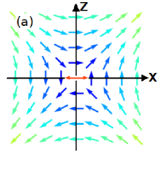
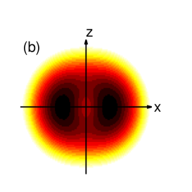
Figure 1: (a) Schematic of a magnetic field quadrupole distribution [equation (1)] and the RF coupling field. The horizontal double-headed arrow (red) indicates the polarization of the coupling RF field. The offset field $B_{0}$ points out of the page. (b) Contours of a typical RF dressed double well potential. (c) Potential energy along $y=0$ (the $x$-axis) in panel (b). Parameters characterizing the double well are defined as: well position $x_{w}$, inter-well barrier height $h$ and well frequency $\omega$.

In the following we first review the theory of the Zeeman effect in non-linear situations (section 2) and then apply the results to RF dressing in the strong field regime (section 3). We report on the effects on both the vibrational frequency of RF dressed atom traps and their locations, and then the paper concludes in section 4.

2 Zeeman shift theory

In the limit of slow atomic motion, the magnetic moment of the atoms keeps its orientation relative to a spatially varying magnetic field, $\bm{B}_{DC}$. The dynamics can be described by the Hamiltonian [36, 37]

$$H=A\bm{I}\cdot\bm{J}+\mu_{B}|\bm{B}_{DC}|(g_{J}J_{z}-g_{I}^{\prime}I_{z}),$$ (2)

where $A$ is a measure of the hyperfine splitting, $\bm{J}$ and $\bm{I}$ are the spin and nuclear angular momentum operators, and the electronic and nuclear $g$-factors are $g_{J}$ and $g_{I}^{\prime}$, respectively. The Bohr magneton is denoted by $\mu_{B}$, as usual.

As is well known, the operator $F_{z}=J_{z}+I_{z}$ commutes with the Hamiltonian (2) and thus $m_{F}$ is a good quantum number (along with $I$ and $J$). Since we consider ⁸⁷Rb with $I=3/2$ and $J=1/2$, the interaction mixes pairs of states $|m_{F}-1/2,1/2\rangle$ and $|m_{F}+1/2,-1/2\rangle$ in a $m_{I}$, $m_{J}$ basis: $|m_{I},m_{J}\rangle$. These two states have the same value of $m_{F}$ by construction. In this case, because $J=1/2$, the diagonalization of Hamiltonian (2) reduces to $2\times 2$ matrix blocks and some uncoupled terms. This leads to a Breit-Rabi formula for the hyperfine energy spectrum of an alkali atom in a magnetic field [36]:

$$E^{Z,\pm}_{m_{F}} = -\frac{A(1+4\alpha g_{I}^{\prime}m_{F})}{4}$$ (3)

$$\pm\frac{A}{2}\sqrt{I(I+1)+\frac{1}{4}+2m_{F}\alpha(g_{J}+g_{I}^{\prime})+\alpha^{2}(g_{J}+g_{I})^{2}}$$

where $\alpha=\mu_{B}|\bm{B}_{DC}|/A$. However, there are two uncoupled states in the $m_{I}$, $m_{J}$ basis: $|I,1/2\rangle$ and $|-I,-1/2\rangle$. These states have energies

$$E^{Z,\pm}_{m_{F}=\pm(I+1/2)} = \frac{A}{2}I\pm\frac{\alpha A}{2}\left(g_{J}-2g_{I}^{\prime}I\right)\,.$$ (4)

In the weak field regime, corresponding to $\alpha\ll 1$, the Zeeman shifts become linear in $|\bm{B}_{DC}|$ and all these energy levels [equation (3) and equation (4)] are approximated by (see e.g. Ref. [37])

$$E^{Z,\pm}_{m_{F}} \approx -\frac{A}{4}+\frac{A}{2}(I+1/2)+m_{F}\mu_{B}g_{F}|\bm{B}_{DC}|,\,.$$ (5)

Here the signs in front of the square root contribution in equation (3) have been absorbed by the definition of the $g$-factor associated with the total angular momentum $\bm{F}=\bm{I}+\bm{J}$. Because $J=1/2$ there are only two possible values $F=I+J=2$ and $F=|I-J|=1$:

$$g_{F} = g_{J}\frac{F(F+1)-I(I+1)+J(J+1)}{2F(F+1)}$$ (6)

$$-g_{I}^{\prime}\frac{F(F+1)+I(I+1)-J(J+1)}{2F(F+1)}\,.$$

Figure 2(a) shows the atomic energy levels, corresponding to the upper hyperfine manifold, at different positions in the field distribution equation (1). In the case of RF dressed atom traps with ⁸⁷Rb atoms in the trapping states $m_{F}=1,2$ follow such energy curves adiabatically and become trapped at positions of minimum field amplitude [16].

Figure 2: (a) Zeeman shifts for the upper manifold ($F=2$) of the ground state of ⁸⁷Rb, in a field distribution as equation (1). Arrows indicate locations of resonance at low (left) and high (right) field intensities. Panels (b) and (c) show dressed potentials (solid) and bare states (dashed) for resonance located at (b) $x_{w}=10\mu$m, with $\omega_{RF}/2\pi=2.63$ MHz and (c) $x_{w}=100\mu$m with $\omega_{RF}/2\pi=15.99$ MHz. Notice how, at large fields, the crossings of bare states have separated in space and in energy (dashed lines). In all cases the field gradient is $G=22.67$ T/m, the RF amplitude is $B_{RF}=357$ mG, and the offset field is $B_{0}=3$ G.

3 Double well dressed potential

We consider a magnetic trap with static field distribution (1), dressed by a uniform and linearly polarized oscillating magnetic field (RF) [4, 1]. The coupling between atomic states is dominated by the component of the RF field orthogonal to $\bm{B}_{DC}$ [5], vanishing at positions where they are parallel (e.g. at positions of coordinates $(x=0,y)$). A typical resulting double well potential is shown in figure 1(b). To characterize the potential energy, we evaluate the dressed energy along the $x$ axis, where a double well appears as a consequence of the dressing.

We define the $z$-axis parallel to direction of the static field, take the RF field polarized along the $x$-axis and apply the standard rotating wave approximation (RWA). Then, the Hamiltonian (2) in a rotating frame becomes

$$H=A\bm{I}\cdot\bm{J}+\mu_{B}|\bm{B}_{DC}|(g_{J}J_{z}-g_{I}^{\prime}I_{z})\pm\hbar\omega_{RF}(J_{z}+I_{z})+\frac{\mu_{B}|\bm{B}_{RF}|}{2}(g_{J}J_{x}-g_{I}^{\prime}I_{x}).$$ (7)

Because $J=1/2$ the sign $\pm$ is chosen according to which hyperfine manifold we are interested in: $F=I+J$ or $F=|I-J|$. This is because each polarization component of the dressing field couples magnetic sublevels within a subspace with a given total angular momentum (A). The diagonalization of equation (7) produces the dressed state energies displayed in figure 3 (solid curve) for the magnetic field configuration of this paper.

In the weak field regime and for RF frequencies much smaller than the hyperfine splitting ($\omega_{RF}\ll A/\hbar$), the dressed energies for states of the upper hyperfine manifold are [1]

$$E^{+}_{m_{F}}\approx-\frac{A}{4}+\frac{A}{2}(I+1/2)+m_{F}\sqrt{(\mu_{B}g_{F}|\bm{B}_{DC}|-\hbar\omega_{RF})^{2}+(\mu_{B}g_{F}|\bm{B}_{RF}|/2)^{2}},$$ (8)

which produces, for the field distribution of equation (1) and for weak-field seeker states [16], the dressed potentials shown in figure 3 (dashed line). The double well is conveniently described by three parameters: the well minimum position ($x_{w}$), the height of the inter-well barrier ($h$) and the well frequency $\omega$ which is defined through a harmonic approximation centred around the potential minimum [see figure 1(c)]. To distinguish these properties being evaluated according to equation (8) or equation (7), we denote the former quantities (i.e. from the weak field expression) with a superscript $0$. (For example, the well position is $x_{w}^{0}$ in the linear regime, and $x_{w}$ more genrally.)

The potential well’s position and frequency are determined by the location of the resonant coupling, as suggested in figure 2(b)-(c), and by the intensity of the RF field. Figure 3 shows typical dressed potentials in a double-well regime (where we show only one of the two wells). We compare both the dressed eigenvalue of Hamiltonian (7), and equation (8) for different RF frequencies $\omega_{RF}$. A rather significant change in the well shape is seen for quite modest well separations for this field gradient. (The well separation is $2x_{w}$ in figure 3.)

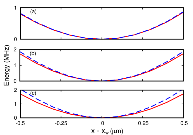
Figure 3: Comparison of non-linear and linear dressed potentials. There are two potential wells at $\pm x_{w}$ and we show here just the well located at $x=+x_{w}$ with $m_{F}=2$: Red (solid) eigenvalue of Hamiltonian (7). Blue (dashed) line is the adiabatic potential (8). The dressing frequencies and well positions are (a) $2.6$ MHz, $x_{w}=10\ \mu$m (b) $5.2$ MHz, $30\ \mu$m and (c) $8.2$ MHz, $50\ \mu$m. The quadrupole field gradient is $G=22.67$ T/m [34] and the bias field is $B_{0}=3.0$ G as in figure 2. In each of (a-c), $\omega_{RF}$ has been adjusted to produce a minimum at the specified value of $x_{w}$.

With a fixed static field configuration, the distance between the wells is controlled by the RF frequency $\omega_{RF}$. At large distances, the non-linear character of Zeeman shifts impacts on the dressed potential, and equation (8) is no longer valid. In particular, the well frequency is significantly modified, as seen for $m_{F}=2$ in figure 4. For well separations of 30 microns, the correction to frequency is about $5\%$ for offset fields of $1$ G (or $3$ G). The relative effect on the frequency increases approximately linearly with the well separation, and can become a significant fraction of $w$ for separations of tens of microns. The weakening of the well (or equivalently, the reduction of $w$), can be qualitatively understood as a consequence of the appearance of multiple resonant positions due to non-linearity of Zeeman shifts [see figure 2(b)]: as the distance between bare state crossings increases, the dressed potential softens in comparison with the potential from a single resonant position. This becomes one of the main effects of the non-linear Zeeman effect on dressed RF potentials.

Figure 5 shows similar results for what is the $F=1$ manifold in the weak field regime. However, in this case we see that the trap is tightened by the non-linear Zeeman effect. The result is understood from the fact that $g_{F}$, equation (6), changes sign for $F=1$. As a result the sequence of levels seen for $F=2$ in figure 2(c) is reversed, which enables us to have tighter trapping as seen (inverted) at the bottom of the manifold of figure 2(c) (and see also figure 5(b) inset). Since the trapping on ⁸⁷Rb $F=2$ involves potentials twice as steep as those on ⁸⁷Rb $F=1$ we would not expect the trap to become tighter in $F=1$ overall. (The factor two in steepness is because the two manifolds have the same magnitude of $g_{F}$, which means a factor of two in the potentials because for $F=2$ we can use $m_{F}=2$, while for $F=1$ we can only use $m_{F}=-1$.) However, figures 4 and 5 show that, in absolute terms, that $F=1$ trap does become tighter than the $F=2$ trap for quite modest values of the RF frequency. In essence, the weakening of the $F=2$ trap by the non-linear Zeeman effect, and corresponding tightening of $F=1$, becomes sufficient for the trap frequency in $F=1$ to become higher.

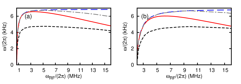
Figure 4: Well frequency as a function of RF frequency, obtained from the eigenvalue of Hamiltonian (7) (solid) and the linear approximation to the eigenvalues (8) (dashed), for (a) $B_{0}=1.0$ G and (b) $B_{0}=3.0$. Other parameters are as in figure 2 (including $F=2$, $m_{F}=2$). The well frequency corresponding to a three level system and its value scaled by $\sqrt{2}$ are shown by the short-dash and dot-dash lines, respectively.

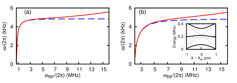
Figure 5: Well frequency as a function of RF frequency in the case $F=1$, $m_{F}=-1$. Results are obtained from the eigenvalue of Hamiltonian (7) (solid) and the linear approximation to the eigenvalues (8) (dashed), for (a) $B_{0}=1.0$ G and (b) $B_{0}=3.0$. Other parameters are as in figure 2. Inset: dressed potentials for the case of $F=1$.

The potential well’s frequency for the dressed state $|F=1,m_{F}=-1\rangle$ can be evaluated analytically using the solution of a three level system (see B), and approximating the well’s position by taking the positions of the resonant couplings (large dots in figure 2(c)) and averaging them. The frequency obtained following this procedure coincides very closely with the numerical results shown in figure 5.

In the case of $F=2$, we find that, similarly, the well frequency corresponding to the dressed state $|F=2,m_{F}=2\rangle$ can be estimated by considering couplings between the bare levels $|F=2,m_{F}=-1\rangle,|F=2,m_{F}=0\rangle$ and $|F=2,m_{F}=1\rangle$. This is shown in figure 4 (short-dash) and indicates that at high RF frequencies the curvature of the dressed energy is dominated by the crossings of just these three levels (see figure 2(c)). In the intermediate regime of dressing frequency, the coupling of all levels contribute significantly to the dressed state and the three level approximation is not valid. However, at low RF dressing frequencies, we observe that the linear regime result coincides with the three level estimate of the well frequency scaled by $\sqrt{2}$ (dash and dash-dot line in figure 4, respectively).

Figure 6 presents a comparison of the non-linear effects on the well position ($\Delta x_{w}=x_{w}-x_{w}^{0}$) and inter-well barrier height ($\Delta h=h-h^{0}$). Again, these are calculated from the diagonalization of the Hamiltonian (7) and by comparing results to the weak field approximation, equation (8). We see that the shift in the position of a potential well can be large in both the low RF frequency limit and the high RF frequency limit (see figure 6(a), inset). The shift at high RF frequency seems reasonable as the higher frequencies usually result in RF resonance in regions of stronger magnetic fields where the non-linear Zeeman effect is expected to play a role. Note here that the vertical asymptotes in figure 6 correspond to the threshold were the RF frequency is just sufficient to excite transitions in the static field configuration, i.e.  $\hbar\omega_{RF}\rightarrow\mu_{B}g_{F}|B_{0}|$.

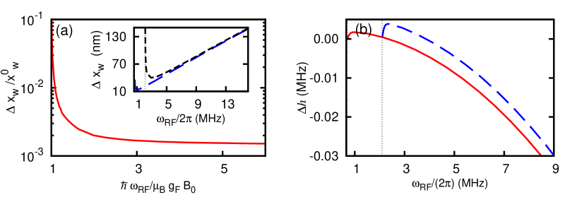
Figure 6: (a) Main panel: Relative displacement of well positions ($\Delta x_{w}/x^{0}_{w}=(x_{w}-x^{0}_{w})/x^{0}_{w}$) versus $\hbar\omega_{RF}/\mu_{B}B_{0}$, evaluated via equation (7). On this scale, $\Delta x_{w}/x^{0}_{w}$ are approximately independent of $B_{0}$. Inset: Well position displacement for offset field $B_{0}=1$ G (dashed) and $B_{0}=3$ G (short-dashed) (b) Modification of the double well barrier height ($\Delta h=h-h^{0}$) for $B_{0}=1$ G (solid) and $B_{0}=3$ G (dashed) respectively, as function of the RF frequency. In all cases $B_{RF}=357$ mG and $G=22.67$ T/m [34]. Dashed vertical lines indicate the limiting frequencies at $\mu_{B}g_{F}B_{0}/h$.

To understand the shifts in position of the potential wells we look carefully at the issue of how we define the resonance location and the potential well location. Shifts of the well positions, $\Delta x_{w}=(x_{w}-x^{0}_{w})$, can be understood by investigating where resonant RF coupling occurs, i.e, positions where $\hbar\omega_{RF}$ matches the energy separation between levels with $|\Delta m_{F}|=1$. That is,

$$E^{Z,+}_{m_{F}}-E^{Z,+}_{m_{F}\pm 1}=\hbar\omega_{RF}$$ (9)

which, in the weak field regime, reduces to a unique value of $\omega_{RF}$ given by

$$\mu_{B}g_{F}|\bm{B}_{DC}|-\hbar\omega_{RF}=0.$$ (10)

In the regime of weak magnetic field, multiple resonances occur at the same position [see figure 2(b)], since the spacing between adjacent sub-levels is degenerate. In contrast, for large fields the degeneracy of transition frequencies is destroyed and the resonance locations become separated in space, as shown in figure 2(c). As in the treatment of the well frequencies above, a simple and good estimate for the location of the potential well minimum $x_{w}$ can be found by taking an average of the positions where equation (9) is satisfied for different $(m_{F},m_{F}\pm 1)$ pairs [dots in figure 2(c)]. This quantity, $\bar{x}_{w}$, has been evaluated using both the procedure of Appendix B (equation 21), and by using the numerical solution of equation (9) itself. These results agree with the full solution of equation (7) and are presented as one curve in figure 6.

4 Conclusions

Our calculations show that for a resonant RF dressed double well potential, the well frequency is a sensitive parameter to the non-linearity of Zeeman shifts. This is relevant for investigations of tunnelling processes in double well potentials, BEC interferometry, and phase coherence dynamics, since these phenomena are sensitive to the potential shape [32, 35]. These modifications of the well frequency can be large enough to be tested experimentally via interferometry or atom cloud oscillations [3, 4].

We have also seen that in taking account of the non-linear Zeeman effect the sign of the $g$-factor is an important consideration in the tightness of the resonantly RF dressed atom trap. In the case of ⁸⁷Rb we found that for modest RF frequencies the $F=1$ dressed trap could be tighter than the $F=2$ dressed trap, which is quite against expectation in the linear regime. By using a model 3-level system, we calculate the well’s frequency for $F=1$. In the case of the $F=2$ manifold, this model works well in a regime of non-linear Zeeman shift. However, the presence of tighter trapping in $F=1$ seems counter-intuitive, not least because the key states of $m_{F}=\pm 1$ do not directly couple. However, the cases we have examined have sufficiently strong coupling that all the levels are mixed by the interaction even though the crossings are seen to be separated in figure 2c.

Finally, we note that near the limiting frequency set by the static offset field (see figure 6), the double well separation and frequency of the dressed potential are quite sensitive to the dressing frequency $\omega_{RF}$ (see also figures 4 and 5). This regime is relevant for double wells with sub-micron separations, a situation likely to occur in near surface trapping configurations [30]. Our work shows that to achieve stable configurations with small well separations, good control of the RF frequency is needed. However, the main result of this work is that the vibrational frequency can be sensitive to the chosen RF frequency because of the non-linear nature of Zeeman shifts.

Appendix A RF dressing in the strong field regime

An alkali atom interacting with a static magnetic field plus an orthogonal RF dressing field is described by the Hamiltonian:

$$H=A\bm{I}\cdot\bm{J}+\mu_{B}|\bm{B}_{DC}|(g_{J}J_{z}-g_{I}^{\prime}I_{z})+\mu_{B}|\bm{B}_{RF}|(g_{J}J_{x}-g_{I}^{\prime}I_{x})\cos(\omega_{RF}t)$$ (11)

where the first term arises from the hyperfine interaction. Assuming that the hyperfine coupling is stronger than the interaction with the static field, the state space can be split into a direct sum of spaces with two angular momentum operators $F^{\downarrow}$ (which has spin $I-J$) and $F^{\uparrow}$ (which has spin $I+J$). Left and right circular polarization components of a linearly polarized dressing field couple magnetic levels within only one of the hyperfine subspaces. Thus, the relevant component in each case is selected by an observer rotating in an appropriate sense. With this in mind, the unitary transformation between lab and rotating frames can be defined by [38]:

$$U=\exp(-i\omega_{RF}t(F_{z}^{\uparrow}-F_{z}^{\downarrow}))\,,$$ (12)

where $F_{z}^{\uparrow}$ and $F_{z}^{\downarrow}$ work in subspaces of $\mathbf{F}$ as described above. Then, in the rotating frame, the time evolution follows the Schrödinger equation $i\hbar\partial_{t}|\psi\rangle=H^{\prime}|\psi\rangle$ with

$$H^{\prime}=U^{\dagger}HU-i\hbar U^{\dagger}\dot{U}.$$ (13)

The hyperfine term and the interaction with the static field are invariant under the unitary transformation equation (12). The interaction with the dressing field transforms into:

$$H^{\prime}_{RF} = \frac{\mu_{B}B_{RF,x}}{2}(g_{J}J_{x}-g_{I}^{\prime}I_{x})$$ (14)

$$+\frac{\mu_{B}B_{RF,x}}{2}(\cos 2\omega_{RF}t\ \hat{x}\mp\sin 2\omega_{RF}t\ \hat{y})\cdot(g_{J}\bm{J}-g_{I}^{\prime}\bm{I}).$$

Neglecting the rapidly rotating field (rotating with angular velocity of $2\omega_{RF}$), the total Hamiltonian becomes the expression given in equation (7).

Appendix B Frequency and position of strong-field potential wells

Consider the dressed energy as function of the static magnetic field, as given, e.g. in equation (8), and produce a Taylor expansion around the minimum occurring at the magnetic field $|\bm{B}_{DC,min}|$,

$$E(|\bm{B}_{DC}|)=E_{0}+\frac{\beta}{2}(|\bm{B}_{DC}|-|\bm{B}_{DC,min}|)^{2}+\ldots$$ (15)

with $\beta$,

$$\beta=\left.\frac{d^{2}E(|\bm{B}_{DC}|)}{d|\bm{B}_{DC}|^{2}}\right|_{|\bm{B}_{DC,min}|}.$$ (16)

The well’s frequency is parametrized by a quadratic dependence of the dressed energy with the distance to the position of minimum

$$E(x)=E_{0}+\frac{mw^{2}}{2}(x-x_{w})^{2}$$ (17)

where

$$|\bm{B}_{DC,min}|=|\bm{B}_{DC}(x_{w})|.$$ (18)

In the case of a quadrupole magnetic field of gradient $G$ plus offset field, where the field is $|\bm{B}_{DC}(x)|=\sqrt{(Gx)^{2}+B_{0}^{2}}$, the well’s frequency in terms of expansion equation (15) is given by:

$$w=\sqrt{\frac{\mu_{B}^{2}\beta}{mA}}G\sqrt{1-\frac{B_{0}}{|\bm{B}_{DC,min}|}}.$$ (19)

Then in the regime of linear Zeeman shifts, and after a Taylor expansion to second order of equation (8) we obtain

$$|\bm{B}_{DC,min}| = \frac{\hbar\omega_{RF}}{g_{F}\mu_{B}}$$

$$\beta = \frac{8Ag_{F}}{\mu_{B}|\bm{B}_{RF}|}.$$ (20)

For this to be valid, the minimum should occur at a magnetic field such that $\mu_{B}|\bm{B}_{DC,min}|\ll 2A$.

For more intense fields, where the multi-level crossing degeneracy is lifted, but levels can still grouped in manifolds $F=I+J$ and $F=|I-J|$, $|\bm{B}_{DC,min}|$ can be obtained as an average of the crossing points between consecutive $m_{F}$ levels. The field at which such crossings occur can be obtained analytically by solving equation (9), expanding the Zeeman shifted energies (3) up to second order in $\mu_{B}B/A$. This procedure gives us

$$|\bm{B}_{DC,min}|=\frac{A}{2F\mu_{B}}\sum_{m_{F}=-F}^{m_{F}=F-1}\frac{g_{F}-\sqrt{g_{F}^{2}\mp 4(1-2m_{F})G_{F}\frac{\hbar\omega_{RF}}{A}}}{2(1-2m_{F})G_{F}}$$ (21)

with

$$G_{F} = \mp\frac{1}{I+1/2}\left(\frac{g_{J}-g_{I}}{2(I+1/2)}\right)^{2}.$$ (22)

In equations (21)-(22) the upper and lower signs are chosen according to $F=I+J$ and $F=|I-J|$ respectively.

Analytic expressions for the dressed energy can only be obtained in simple cases. For our example of ⁸⁷Rb in its ground state, after ignoring couplings between the $F=I+J$ and $F=|I-J|$, the dressed energies of the $F=1$ manifold are:

$$E_{i}(|\bm{B}_{DC}|)=-\frac{C}{3}+\frac{2\sqrt{C^{2}-3D}}{3}\cos\left(\frac{\theta+\phi_{i}}{3}\right)+A\left(-\frac{1}{4}+\frac{g_{F}}{2|g_{F}|}(I+0.5)\right)$$ (23)

with $\phi_{i}=0,2\pi,4\pi$ corresponding to $i=1,2,3$, and

$$C = -(E^{Z,-}_{1}+E^{Z,-}_{0}+E^{Z,-}_{1})$$

$$D = E^{Z,-}_{1}E^{Z,-}_{-1}+E^{Z,-}_{1}E^{Z,-}_{0}+E^{Z,-}_{-1}E^{Z,-}_{0}-2d^{2}+\hbar\omega_{RF}(E^{Z,-}_{1}-E^{Z,-}_{-1}-\hbar\omega_{RF})$$

$$E = d^{2}(E^{Z,-}_{1}+E^{Z,-}_{-1})-E^{Z,-}_{1}E^{Z,-}_{0}E^{Z,-}_{-1}-\hbar\omega_{RF}E^{Z,-}_{0}(E^{Z,-}_{1}-E^{Z,-}_{-1}-\hbar\omega_{RF})$$

$$R = (9CD-27E-2C^{3})/54$$

$$Q = (3D-C^{2})/9$$

$$\theta = \arccos(R/\sqrt{-Q^{3}}),$$ (24)

where $d=\frac{\mu_{B}B_{RF}g_{F}}{2}\langle m_{F}\pm 1|J_{x}+I_{x}|m_{F}\rangle$ and the Zeeman shifted levels are given by equation (3).

References

References

- [1] Zobay O and Garraway B M 2001 Phys. Rev. Lett. 86(7) 1195
- [2] Zobay O and Garraway B M 2004 Phys. Rev. A 69(2) 023605
- [3] Colombe Y, Knyazchyan E, Morizot O, Mercier B, Lorent V and Perrin H 2004 Europhysics Letters 67 593
- [4] Schumm T, Hofferberth S, Andersson L M, Wildermuth S, Groth S, Bar-Joseph I, Schmiedmayer J and Krüger P 2005 Nature Physics 1 57
- [5] Lesanovsky I, Schumm T, Hofferberth S, Andersson L M, Krüger P and Schmiedmayer J 2006 Phys. Rev. A 73(3) 033619
- [6] Garrido Alzar C L, Perrin H, Garraway B M and Lorent V 2006 Phys. Rev. A 74(5) 053413
- [7] Jo G B, Shin Y, Will S, Pasquini T A, Saba M, Ketterle W, Pritchard D E, Vengalattore M and Prentiss M 2007 Phys. Rev. Lett. 98(3) 030407
- [8] Sewell R J, Dingjan J, Baumgärtner F, Llorente-García I, Eriksson S, Hinds E A, Lewis G, Srinivasan P, Moktadir Z, Gollasch C O and Kraft M 2010 Journal of Physics B: Atomic, Molecular and Optical Physics 43 051003
- [9] Baumgärtner F, Sewell R J, Eriksson S, Llorente-García I, Dingjan J, Cotter J P and Hinds E A 2010 Phys. Rev. Lett. 105(24) 243003
- [10] Krüger P, Hofferberth S, Mazets I E, Lesanovsky I and Schmiedmayer J 2010 Phys. Rev. Lett. 105(26) 265302
- [11] Cronin A D, Schmiedmayer J and Pritchard D E 2009 Rev. Mod. Phys. 81(3) 1051
- [12] Metcalf H and van der Straten P 1999 Laser Cooling and Trapping (Springer-Verlag New York, Inc.)
- [13] Reichel J and Vuletic V (eds) 2011 Atom Chips (Wiley VCH)
- [14] Lundblad N, Lee P J, Spielman I B, Brown B L, Phillips W D and Porto J V 2008 Phys. Rev. Lett. 100(15) 150401
- [15] Shotter M, Trypogeorgos D and Foot C 2008 Phys. Rev. A 78(5) 051602
- [16] Fortägh J and Zimmermann C 2007 Rev. Mod. Phys. 79 235
- [17] Lesanovsky I and von Klitzing W 2007 Phys. Rev. Lett. 99(8) 083001
- [18] Fernholz T, Gerritsma R, Krüger P and Spreeuw R J C 2007 Phys. Rev. A 75(6) 063406
- [19] Heathcote W H, Nugent E, Sheard B T and Foot C J 2008 New Journal of Physics 10 043012
- [20] Gildemeister M, Sherlock B E and Foot C J 2012 Phys. Rev. A 85(5) 053401
- [21] Gildemeister M, Nugent E, Sherlock B E, Kubasik M, Sheard B T and Foot C J 2010 Phys. Rev. A 81(3) 031402
- [22] Sherlock B E, Gildemeister M, Owen E, Nugent E and Foot C J 2011 Phys. Rev. A 83(4) 043408
- [23] Morizot O, Garrido Alzar C L, Pottie P E, Lorent V and Perrin H 2007 Journal of Physics B: Atomic, Molecular and Optical Physics 40 4013
- [24] Easwaran R K, Longchambon L, Pottie P E, Lorent V, Perrin H and Garraway B M 2010 Journal of Physics B: Atomic, Molecular and Optical Physics 43 065302
- [25] Morgan T, O’Sullivan B and Busch T 2011 Physical Review A 83 053620
- [26] White M, Gao H, Pasienski M and DeMarco B 2006 Phys. Rev. A 74(2) 023616
- [27] Morizot O, Longchambon L, Kollengode Easwaran R, Dubessy R, Knyazchyan E, Pottie P E, Lorent V and Perrin H 2008 The European Physical Journal D - Atomic, Molecular, Optical and Plasma Physics 47(2) 209
- [28] Morizot O, Colombe Y, Lorent V, Perrin H and Garraway B M 2006 Phys. Rev. A 74(2) 023617
- [29] Folman R 2011 Quantum Information Processing 10(6) 995
- [30] Allwood D A, Schrefl T, Hrkac G, Hughes I G and Adams C S 2006 Appl. Phys. Lett. 89 014102
- [31] Sinuco-León G, Kaczmarek B, Krüger P and Fromhold T M 2011 Phys. Rev. A 83(2) 021401
- [32] LeBlanc L J, Bardon A B, McKeever J, Extavour M H T, Jervis D, Thywissen J H, Piazza F and Smerzi A 2011 Phys. Rev. Lett. 106(2) 025302
- [33] van Es J J P, Whitlock S, Fernholz T, van Amerongen A H and van Druten N J 2008 Phys. Rev. A 77(6) 063623
- [34] Hofferberth S, Fischer B, Schumm T, Schmiedmayer J and Lesanovsky I 2007 Phys. Rev. A 76(1) 013401
- [35] Ottaviani C, Ahufinger V, Corbalán R and Mompart J 2010 Phys. Rev. A 81(4) 043621
- [36] Corney A 1977 Atomic and Laser Spectroscopy (Oxford)
- [37] Foot C J 2008 Atomic Physics (Oxford University Press)
- [38] Mischuck B E, Merkel S T and Deutsch I H 2012 Phys. Rev. A 85(2) 022302