Lattice density functional theory at finite temperature with strongly density-dependent exchange-correlation potentials

Abstract

The derivative discontinuity of the exchange-correlation (xc) energy at integer particle number is a property of the exact, unknown xc functional of density functional theory (DFT) which is absent in many popular local and semilocal approximations. In lattice DFT, approximations exist which exhibit a discontinuity in the xc potential at half filling. However, due to convergence problems of the Kohn-Sham (KS) self-consistency cycle, the use of these functionals is mostly restricted to situations where the local density is away from half filling. Here a numerical scheme for the self-consistent solution of the lattice KS Hamiltonian with a local xc potential with rapid (or quasi-discontinuous) density dependence is suggested. The problem is formulated in terms of finite-temperature DFT where the discontinuity in the xc potential emerges naturally in the limit of zero temperature. A simple parametrization is suggested for the xc potential of the uniform 1D Hubbard model at finite temperature which is obtained from the solution of the thermodynamic Bethe ansatz. The feasibility of the numerical scheme is demonstrated by application to a model of fermionic atoms in a harmonic trap. The corresponding density profile exhibits a plateau of integer occupation at low temperatures which melts away for higher temperatures.

I Introduction

Originally, static (ground-state) density functional theory (DFT) has been formulated HohenbergKohn:64 ; KohnSham:65 for many-electron systems in the continuous space of three spatial dimensions with the electrons interacting via the Coulomb interaction. On the other hand, many phenomena in many-particle physics are studied in terms of model systems on discrete lattices, typically of tight-binding form. The one-dimensional Hubbard model or the Anderson impurity model are just the most prominent examples. Typically, these models are studied with techniques different from DFT. However, DFT can be a useful tool for the investigation of these models as well, especially when one wants to take into account the effects of non-uniform external potentialsGunnarssonSchoenhammer:86 ; LimaSilvaOliveiraCapelle:03 ; XianlongPoliniTosiCampoCapelleRigol:06 ; MaPilatiTroyerDai:12 . For example, cold atoms in optical lattices confined in an harmonic trap may very well be modelled by a lattice model with confining external potential where the particles interact through a Hubbard-type interaction Review .

The idea of formulating DFT for electrons on a lattice of sites has been pioneered by Schönhammer and coworkers GunnarssonSchoenhammer:86 ; SchoenhammerGunnarssonNoack:95 . As with usual DFT, the applicability and success of lattice DFT hinges on the availability of approximations to the unknown exchange-correlation (xc) functional. Capelle and coworkers proposed a local functional for the xc energy per site based on the Bethe-ansatz solution of the uniform 1D Hubbard model at zero temperature LimaSilvaOliveiraCapelle:03 ; SilvaLimaMalvezziCapelle:05 . Thus, for one-dimensional lattice models, the 1D Hubbard model takes the role of the uniform electron gas in continuum formulation of DFT as an exactly solvable model system which provides the essential input for the construction of the local approximation. In the same spirit, xc functionals have been suggested based on other Hubbard lattice models such as the two-dimensional hexagonal lattice IjaesHarju:10 or the simple cubic lattice in 3D KarlssonPriviteraVerdozzi:11 .

An interesting property of the Bethe-ansatz local density approximation (BALDA) in 1D (and also its counterparts for 2D or 3D lattice models) is its discontinuous form of the xc potential at half filling or integer occupation LimaOliveiraCapelle:02 . Physically, this discontinuity is a direct consequence of the Mott-Hubbard gap of the Hubbard model while in the DFT context it is nothing but the well-known derivative discontinuity of the xc energy at integer particle number at zero temperature PerdewParrLevyBalduz:82 .

The BALDA has been successfully applied to spatially inhomogeneous Hubbard supperlattices SilvaLimaMalvezziCapelle:05 , to cold fermionic atoms in a harmonic trap, both with repulsive XianlongPoliniTosiCampoCapelleRigol:06 and attractive XianlongRizziPoliniFazioTosiCampoCapelle:07 electronic interaction and to the study of the static and dynamic linear density response SchenkDzierzawaSchwabEckern:08 ; AkandeSanvito:10 . Extensions of the BALDA have been suggested to systems in static magnetic fields AkandeSanvito:12 and, in the adiabatic form, to the domain of time-dependent DFT Verdozzi:08 where it has been used to study the dynamics of finite Hubbard clusters. Recently the adiabatic BALDA has been applied to describe the time evolution of trapped 1D lattice fermions in the Mott insulator regime KarlssonVerdozziOdashimaCapelle:11 . A modified version of the BALDA has been used in the study of time-dependent transport through an Anderson impurity KurthStefanucciKhosraviVerdozziGross:10 where the discontinuity has been related to Coulomb blockade.

From a physical point of view the discontinuity at integer particle number is certainly a desirable property for an approximation to have, at least at zero temperature. As we will argue below, the zero-temperature discontinuity may be viewed as the zero temperature limit of a continuous xc potential at finite temperature. From a practical point of view, if a local discontinuous (or rapidly varying) xc potential is used, one often faces convergence problems of the Kohn-Sham (KS) self-consistency cycle XianlongPoliniTosiCampoCapelleRigol:06 essentially whenever the local density is close to integer occupation.

In the present work we propose a practical solution to this convergence problem by viewing it as an equivalent problem of finding the solution to a coupled set of nonlinear equations. In Sec. II, we start with a general discussion of the KS self-consistency cycle and possible convergence problems when using KS potentials which vary rapidly for small variations in the density. The problem is illustrated explicitly on the simple, exactly soluble model system of a single interacting site in contact with a heat and particle bath. In Sec. III, we then introduce the 1D lattice models studied throughout this work and briefly summarize the idea of a local approximation for lattice models which has been discussed in the literature. We will work in the framework of finite-temperature DFT Mermin:65 , and Sec. IV is devoted to the construction of an approximate xc potential for this framework. We construct the xc potential of the uniform 1D Hubbard model for finite temperatures based on the thermodynamic Bethe ansatz. We provide a simple parametrization of this potential using insights gained from the simple single site model discussed earlier. In Sec. V we introduce our algorithm for the practical solution of the self-consistency problem which is based on a multi-dimensional bisection method. In Sec. VI we show a numerical application of the method to the problem of interacting particles in a harmonic trap before we present our conclusions in Sec. VII. In the Appendix we provide explicit expressions for the xc free energy per site for the simple parametrization of the thermodynamic Bethe ansatz solutions to the uniform Hubbard model.

II Kohn-Sham problem with rapidly varying density functionals

The implementation of DFT via the KS method gained enormous popularity because it reduces calculations of the density $n({\bf r})$ in a complicated strongly interacting system to computing $n({\bf r})$ for a reference system of noninteracting KS particles. The KS particles move in the presence of an effective potential $v^{\rm KS}=v+v_{\rm Hxc}[n]$, where $v$ is an external potential and $v_{\rm Hxc}[n]$ is the Hartree-exchange-correlation (Hxc) potential which depends on the density and is adjusted self-consistently to reproduce the physical density distribution of the interacting system. The self-consistent nature of the KS problem makes it nonlinear and thus not absolutely trivial. In fact, the whole point of the present paper is to identify one of the potentially dangerous physical situations and to propose a recipe for its solution.

II.1 KS self-consistency as a fixed point problem: the issue of convergence

Assuming that the potential $v_{\rm Hxc}[n]$ as functional of the density is known, the general KS problem can be formulated as follows. We have to find a set of KS orbitals $\varphi^{(\alpha)}$ and KS energies $\varepsilon_{\alpha}$ by solving a one-particle stationary Schrödinger equation

$$(\hat{t}+v+v_{\rm Hxc}[n])\varphi^{(\alpha)}=\varepsilon_{\alpha}\varphi^{(\alpha)},$$ (1)

where $\hat{t}$ is the one-particle kinetic energy operator. As the operator in Eq. (1) depends on the density we need an additional “self-consistency equation” that relates the set of $\{\varphi^{(\alpha)},\varepsilon_{\alpha}\}$ to $n({\bf r})$. Obviously this equation is simply the standard definition of the density of noninteracting particles

$$n({\bf r})=2\sum_{\alpha}f(\varepsilon_{\alpha})\left|\varphi^{(\alpha)}({\bf r})\right|^{2},$$ (2)

where the factor two comes from spin. $f(\omega)=(1+\exp(\beta(\omega-\mu)))^{-1}$ is the Fermi distribution, $\beta=1/T$ is the inverse temperature, and $\mu$ is the chemical potential which is either given externally or determined by fixing the total number of particles.

Calculation of the density from Eqs. (1)-(2) is equivalent to finding a fixed point of a certain density functional. Indeed, the eigenvalue problem of Eq. (1) defines a map $n\mapsto\{\varphi^{(\alpha)},\varepsilon_{\alpha}\}$ from the density to the set of KS eigenfunctions and eigenvalues, i. e., it determines the functionals $\varphi^{(\alpha)}[n]$ and $\varepsilon_{\alpha}[n]$. Inserting these functionals into Eq. (2) we obtain the following form

$$n=2\sum_{\alpha}f(\varepsilon_{\alpha}[n])\left|\varphi^{(\alpha)}[n]\right|^{2}\equiv G[n],$$ (3)

which is a typical fixed point problem for the functional $G[n]$ on the right hand side.

In practice, the self-consistent KS problem of Eqs. (1)-(2), or equivalently the fixed point problem of Eq. (3), is commonly solved iteratively. In the simplest case one starts with some initial guess $n^{(0)}$ for the density and constructs a sequence of iterations $n^{(k)}$ as follows

$$n^{(0)},\,n^{(1)}=G[n^{(0)}],\dots,\,n^{(k)}=G[n^{(k-1)}],\dots$$ (4)

The limiting point of this sequence presumably gives a self-consistent solution of the KS equation

$$n=\lim_{k\to\infty}n^{(k)}.$$ (5)

Unfortunately the assumed convergence cannot be guaranteed in general, in spite of the fact that the original KS problem definitely has a unique solution. From the Banach fixed point theorem (the contraction mapping principle) we know that the sequence of Eq. (4) does necessarily converge to a unique fixed point if the functional $F[n]$ is contractive, i. e., if the following condition is satisfied

$$\|G[n]-G[n^{\prime}]\|\leq\lambda\|n-n^{\prime}\|,\quad 0<\lambda<1,$$ (6)

where $\|\dots\|$ means a properly chosen norm in the space of densities. Apparently this condition requires $F[n]$ to be a sufficiently smooth functional of the density, which is not always the case. Moreover there are important physical situations where the inequality of Eq. (6) is always violated. To understand this more clearly we estimate the left hand side of Eq. (6) for a small density variation $n^{\prime}=n+\delta n$ with $\delta n\ll n$

$$\|G[n]-G[n^{\prime}]\|\approx\|\chi\frac{\delta v_{\rm Hxc}}{\delta n}(n-n^{\prime})\|$$ (7)

where $\chi$ is the density response function. Obviously the right hand side of Eq. (7) cannot be smaller than $\lambda\|n-n^{\prime}\|$ with $\quad 0<\lambda<1$ if the Hxc potential is a rapidly varying functional of $n$, i. e., if $\frac{\delta v_{\rm Hxc}}{\delta n}$ is large at least for some directions in density space. Physically this should always happen in systems composed of weakly coupled fragments if the number of particles in at least one of the fragments is close to an integer value. Then a density transfer to/from this fragment causes a strong variation of the potential. The origin of this behavior is in the famous discontinuity of the exact xc potential at integer number of particles PerdewParrLevyBalduz:82 . The most prominent examples of systems demonstrating such a behavior are molecules close to dissociation or strongly correlated solids near the Mott-Hubbard transition. In all those systems where the physics is governed by a nearly discontinuous xc potential the standard iterative procedure of solving the KS equations will not converge.

In the next subsection we explicitly illustrate the above general argument by considering a very simple model system – a single lattice site which can host at most two spin-1/2 fermions. The purpose for studying this model is twofold. Firstly, this is probably the only case where the exact xc potential can be found analytically for any temperature. The corresponding KS problem possesses an analytic solution and, because of its simple structure, clearly shows when and why the existing unique fixed point cannot be reached iteratively. Secondly, a single site DFT serves as a paradigmatic example for more general interacting lattice models. In fact, the analytic form of the single site Hxc potential will later be used to construct a simple parametrization for the Hxc potential of the uniform Hubbard model at finite temperatures.

II.2 KS-DFT for a single site model

Let us consider one single-orbital site in contact with a heat and particle bath at inverse temperature $\beta$ and chemical potential $\mu$ StefanucciKurth:11 ; EversSchmitteckert:11 .

The Hamiltonian for this single site model (SSM) in the presence of an on-site interaction is given by

$$\hat{H}_{\rm SSM}=v_{0}\hat{n}_{0}+U\hat{n}_{0,\uparrow}\hat{n}_{0,\downarrow}$$ (8)

where $v_{0}$ is the on-site energy and $U$ is the charging energy, $\hat{n}_{0,\sigma}$ and $\hat{n}_{0}=\sum_{\sigma=\uparrow,\downarrow}\hat{n}_{0,\sigma}$ are the operators for the on-site density with spin $\sigma$ and for the total density, respectively. Similarly, for the non-interacting case the single-site Hamiltonian reads

$$\hat{H}_{\rm SSM}^{s}=v_{s}\hat{n}_{0}$$ (9)

with on-site energy $v_{s}$. The complete Fock space of both Hamiltonians is spanned by the states $|0\rangle$, $|\uparrow\rangle$, $|\downarrow\rangle$, and $|\uparrow\downarrow\rangle$ with particle occupation of zero, one, and two. These states are both eigenstates of $\hat{H}_{\rm SSM}$ with eigenvalues $0$, $v_{0}$, $v_{0}$, and $2v_{0}+U$, as well as eigenstates of $\hat{H}_{\rm SSM}^{s}$ with eigenvalues $0$, $v_{s}$, $v_{s}$, and $2v_{s}$, respectively. For the single site model, the particle number operator is equal to the density operator, $\hat{N}=\hat{n}_{0}$, and the density $n_{0}={\rm Tr}\left\{\hat{\rho}\hat{n}_{0}\right\}$ for the interacting case then reads

$$n_{0}=$$ (10)

$$\frac{2\exp(-\beta(v_{0}-\mu))+2\exp(-\beta(2(v_{0}-\mu)+U))}{Z^{\rm SSM}}$$

where

$$Z^{\rm SSM}=1+2\exp(-\beta(v_{0}-\mu))+\exp(-\beta(2(v_{0}-\mu)+U))$$ (11)

is the grand canonical partition function. Eq. (10) only depends on the quantity $\tilde{v}_{0}=v_{0}-\mu$ and the function $n_{0}(\tilde{v}_{0})$ can be inverted explicitly leading to

$$\tilde{v}_{0}(n_{0})=-U-\frac{1}{\beta}\ln\left(\frac{\delta n+\sqrt{\delta n^{2}+e^{-\beta U}(1-\delta n^{2})}}{1-\delta n}\right)$$ (12)

where $\delta n=n_{0}-1$.

Following the same lines, for the non-interacting case the density reads

$$n_{0}^{s}=\frac{2\exp(-\beta(v_{s}-\mu))+2\exp(-\beta(2(v_{s}-\mu)))}{Z_{s}^{\rm SSM}}$$ (13)

with the non-interacting partition function

$$Z_{s}^{\rm SSM}=1+2\exp(-\beta(v_{s}-\mu))+\exp(-\beta(2(v_{s}-\mu)))\;.$$ (14)

Again, the density $n_{0}^{s}$ only depends on the quantity $\tilde{v}_{s}=v_{s}-\mu$ and one can invert $n_{0}^{s}(\tilde{v}_{s})$ to yield

$$\tilde{v}_{s}(n_{0}^{s})=-\frac{1}{\beta}\ln\left(\frac{1+\delta n^{s}}{1-\delta n^{s}}\right)$$ (15)

with $\delta n^{s}=n_{0}^{s}-1$.

The exact Hxc potential for the SSM can now easily be calculated by requiring that the interacting density equals the non-interacting one $n_{0}=n_{0}^{s}=:n$ and taking the difference of the two expressions (15) and (12), i.e.,

$$v_{\rm Hxc}^{\rm SSM}(n,U,T)=\tilde{v}_{s}(n)-\tilde{v}_{0}(n)=\frac{U}{2}+g(n-1)$$ (16)

where

$$g(x)=\frac{U}{2}+\frac{1}{\beta}\ln\left(\frac{x+\sqrt{x^{2}+e^{-\beta U}(1-x^{2})}}{1+x}\right)$$ (17)

which is easily shown to be an odd function of its argument, $g(-x)=-g(x)$.

In Fig. 1 we show the SSM Hxc potential $v_{\rm Hxc}^{\rm SSM}(n)$ as function of the density for different temperatures. At low temperatures, $v_{\rm Hxc}^{\rm SSM}(n)$ becomes an extremely rapidly varying function of $n$ in the vicinity of $n=1$, approaching a step function with a step of height $U$ at $n=1$ in the limit of zero temperature.

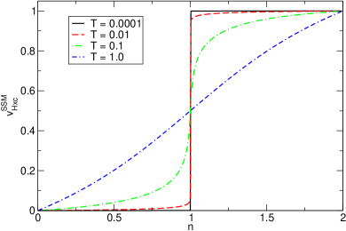
Figure 1: Hartree-exchange-correlation potential of the single-site model for different temperatures $T=1/\beta$. Energies given in units of $U$.

Now, having at hand the exact Hxc potential, we can study the KS problem. In the single site DFT, the general fixed point equation (3) reduces to the following algebraic transcendental equation

$$n=2f\left(v_{0}+v_{\rm Hxc}^{\rm SSM}(n)\right)\equiv G(n).$$ (18)

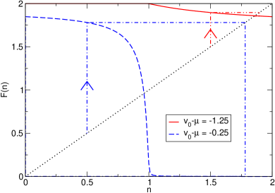
Figure 2: Left-hand side (dotted black line ) and r.h.s. of Eq. (18) for different values of $v_{0}-\mu$ and temperature $T=0.1$. (Energies given in units of $U$.) For given $v_{0}-\mu$, the self-consistent solution is given by the intersection of the corresponding $G(n)$ with the straight line. For $-U<v_{0}-\mu<0$, the iterative scheme $n^{(k+1)}=G(n^{(k)})$, indicated by the dash-dotted lines, does not converge.

This equation can be easily solved analytically. By construction, the solution to Eq. (18) simply returns the function $n(T,\mu)$ defined by Eqs. (10) and (11). In Fig. 2 we show the left (straight line) and right hand sides of Eq. (18) for two different values of $v_{0}-\mu$. Obviously, for a given $v_{0}$ there is only one intersection between $n$ and $G(n)$, which means that the function $G(n)$ always has only one fixed point. However, if the expected solution lies in the region of fast variation of $v_{\rm Hxc}$, i.e. $n\sim 1$, the fixed point cannot be reached by iterations. Independently of the choice of the initial guess, after a few iterations we enter a limiting cycle with the density endlessly jumping between $n\approx 0$ and $n\approx 2$. This behavior is generic for low enough temperatures, $T\ll U$, and the chemical potential in the region $v_{0}<\mu<v_{0}+U$, which are the conditions ensuring that $v_{\rm Hxc}(n)$ has a step-like form (see Fig. 1) and the physical on-site occupation is close to unity. Examples of the iterative cycle are indicated in Fig. 2 showing the convergence of the cycle of Eq. (4) for $v_{0}-\mu=-1.25$, and the lack of convergence for $v_{0}-\mu=-0.25$.

From the discussion in Sec. II.1 it is clear that the same type of non-convergence of the KS iterative sequence should occur in any system with a discontinuous/rapidly varying xc potential. In the rest of this paper we study and solve this problem for lattice models where the discontinuity of $v_{\rm Hxc}$ reflects Mott-Hubbard correlations and can easily be captured at the level of a local density approximation.

III Lattice density functional theory

III.1 Lattice DFT: Formalism and Model

As a particular example of a lattice model, we consider one-dimensional, interacting many-electron systems on a tight-binding lattice described by the Hamiltonian

$$\hat{H} = -t\sum_{i=1}^{N_{s}-1}\sum_{\sigma=\uparrow,\downarrow}\left(\hat{c}_{i,\sigma}^{\dagger}\hat{c}_{i+1,\sigma}+H.c.\right)$$ (19)

$$+U\sum_{i=1}^{N_{s}}\hat{n}_{i,\uparrow}\hat{n}_{i,\downarrow}+\sum_{i=1}^{N_{s}}v_{i}\hat{n}_{i}$$

where $\hat{c}_{i,\sigma}^{\dagger}$ ($\hat{c}_{i,\sigma}$) are the fermionic creation (annihilation) operators for an electron with spin $\sigma$ at site $i$, $\hat{n}_{i,\sigma}=c_{i,\sigma}^{\dagger}c_{i,\sigma}$ and $\hat{n}_{i}=\sum_{\sigma=\uparrow,\downarrow}\hat{n}_{i,\sigma}$ are the operators for the density of electrons with spin $\sigma$ and for the total electron density at site $i$, respectively. The nearest neighbor hopping element is $t$, $U$ is the Hubbard interaction. $v_{i}$ is the external potential at site $i$ and $N_{s}$ is the total number of sites. For simplicity, we consider systems in the absence of magnetic fields. For the grand-canonical ensemble, when the system is in contact with a heat bath at inverse temperature $\beta$ and a particle bath at chemical potential $\mu$, the statistical operator is

$$\hat{\rho}=\frac{1}{Z}\exp(-\beta(\hat{H}-\mu\hat{N}))$$ (20)

where $\hat{N}=\sum_{i=1}^{N_{s}}\hat{n}_{i}$ is the operator for the total number of particles and the grand canonical partition function is $Z={\rm Tr}\left\{\exp(-\beta(\hat{H}-\mu\hat{N}))\right\}$ with the trace over all states of Fock space. In thermal equilibrium, an observable described by the operator $\hat{A}$ then takes the value $A={\rm Tr}\left\{\hat{\rho}\hat{A}\right\}$.

In the spirit of DFT at finite temperatures Mermin:65 , the Hamiltonian (19) is mapped onto the following Hamiltonian of non-interacting electrons

$$\hat{H}^{\rm KS}=-t\sum_{i=1}^{N_{s}}\sum_{\sigma=\uparrow,\downarrow}\left(\hat{c}_{i,\sigma}^{\dagger}\hat{c}_{i+1,\sigma}+H.c.\right)+\sum_{i=1}^{N_{s}}v_{i}^{\rm KS}\hat{n}_{i}$$ (21)

where the effective single particle KS potential $v^{\rm KS}_{i}$ at site $i$ is chosen such that the equilibrium density $n_{i}={\rm Tr}\left\{\hat{\rho}\hat{n}_{i}\right\}$ of the interacting Hamiltonian (19) and the KS Hamiltonian (21) are the same for all sites. The KS potential at site $i$ then has the form

$$v_{i}^{\rm KS}=v_{i}+v_{i}^{\rm Hxc}$$ (22)

where $v_{i}$ is the external potential at site $i$ and, similarly, $v_{i}^{\rm Hxc}$ is the Hxc potential at site $i$. In general, the Hxc potential at site $i$ depends on the equilibrium density at all other sites, i.e., $v_{i}^{\rm Hxc}=v_{i}^{\rm Hxc}(\{n_{j}\})$. Typically, however, the exact form of the Hxc potential is unknown and one has to resort to approximations. Once an approximation to $v_{i}^{\rm Hxc}$ has been specified, the equilibrium density of the KS Hamiltonian $\hat{H}^{\rm KS}$ can be found by self-consistent solution of the KS equation on the lattice

$$\sum_{j=1}^{N_{s}}\left(-t_{ij}+v_{i}^{\rm KS}\delta_{ij}\right)\varphi_{j}^{(\alpha)}=\varepsilon_{\alpha}\varphi_{i}^{(\alpha)}$$ (23)

(with $t_{ij}=t$ for $j=i\pm 1$ and $t_{ij}=0$ otherwise) together with

$$n_{i}=2\sum_{\alpha}f(\varepsilon_{\alpha})|\varphi_{i}^{(\alpha)}|^{2}\;.$$ (24)

III.2 Local density approximations in the lattice DFT

In the local approximation, the Hxc potential at site $i$ only depends on the density at the same site $i$, $v_{i}^{\rm Hxc,loc}=v_{\rm Hxc}^{\rm mod}(n_{i})$. The functional dependence of $v_{\rm Hxc}^{\rm mod}(n)$ on the density is extracted from some interacting model system for which the exact solution can be constructed by analytical and/or numerical techniques. Probably the most prominent example of such a functional for lattice-DFT is the local density approximation (LDA) based on Bethe-ansatz solution of the uniform Hubbard model in 1D (Bethe-ansatz LDA, BALDA) at zero temperature LimaSilvaOliveiraCapelle:03 ; SilvaLimaMalvezziCapelle:05 ; LiebWu:68 .

Strictly speaking, at zero temperature and exactly at half-filling ($n=1$), the BALDA xc potential is not defined since the xc energy per particle is not differentiable at this point. One pragmatic way around this mathematical problem is to smoothen the discontinuity in some ad-hoc manner KurthStefanucciKhosraviVerdozziGross:10 ; KarlssonVerdozziOdashimaCapelle:11 . Alternatively one can construct xc functionals for finite temperature which approach a discontinuous function in the zero temperature limit. We have already followed this route in Sec. II.2 to formulate a single site DFT, and will pursue it further in Sec. IV for the 1D Hubbard model.

Although one can avoid the use of truly discontinuous xc potentials in this way, the resulting KS potentials will still be very rapidly varying functions of the density. This is exactly the property leading to a non-convergence of a simple iterative procedure, a fact which has been recognized in attempts to use the BALDA xc potential within the usual KS self-consistency cycle XianlongPoliniTosiCampoCapelleRigol:06 .

IV Local approximations at finite temperature

In the present Section we propose several versions of a local functional at finite temperature for which the corresponding Hxc potentials exhibit rapid variations as function of the density. This functional is based on the thermodynamic Bethe ansatz (TBA) solution of the uniform Hubbard model in one dimensionTakahashi:72 and is thus an extension of the corresponding work at zero temperature SchoenhammerGunnarssonNoack:95 ; LimaSilvaOliveiraCapelle:03 .

We have numerically solved the coupled integral equations of the TBA following Refs. KawakamiUsukiOkiji:89, ; UsukiKawakamiOkiji:90, ; TakahashiShiroishi:02, . For given inverse temperature $\beta$, the density is calculated as a function of the chemical potential which can be inverted to give the chemical potential as function of the density. For the interacting and non-interacting cases these inverse functions are denoted as $\mu(n)$ and $\mu_{s}(n)$, respectively. From these two functions we obtain the density-dependent Hxc potential of the TBA as

$$v_{\rm Hxc}^{\rm TBA}(n)=\mu(n)-\mu_{s}(n)$$ (25)

In Fig. 3 we show the density dependence of the TBA Hxc potentials for various values of the interaction $U$ and various temperatures $T=1/\beta$. At low temperatures and for sufficiently large values of $U$, the TBA Hxc potential $v_{\rm Hxc}^{\rm TBA}(n)$ exhibits rapid variations around half filling ($n=1$) as function of density. In the zero-temperature limit this feature reduces to a step whose height is given by the Mott-Hubbard gap. This gap can be expressed in terms of the parameters of the model as (from now on all energies are given in units of the hopping matrix element $t$ unless otherwise noted)

$$\Delta_{0}(U)=\frac{16}{U}\int_{1}^{\infty}{\rm d}x\;\frac{\sqrt{x^{2}-1}}{\sinh(2\pi x/U)}$$ (26)

which is nothing but the derivative discontinuity of the uniform Hubbard model at half filling LimaOliveiraCapelle:02 ; LiebWu:68 .

Away from $n=1$, even at low temperatures the dependence of $v_{\rm Hxc}^{\rm TBA}(n)$ on the density is rather slow and smooth. For high temperatures, the sharp feature around half filling is washed out. As a consequence of particle-hole symmetry, the TBA Hxc potential takes the value $U/2$ at $n=1$ for all temperatures and exhibits a point symmetry around this point as function of density, i.e., $v_{\rm Hxc}^{\rm TBA}(n)=U/2+g^{\rm TBA}(n-1)$ with $g^{\rm TBA}(-x)=-g^{\rm TBA}(x)$. Furthermore the values of the TBA Hxc potential at the endpoints of the density interval are $v_{\rm Hxc}^{\rm TBA}(0)=0$ and $v_{\rm Hxc}^{\rm TBA}(2)=U$ for all temperatures.

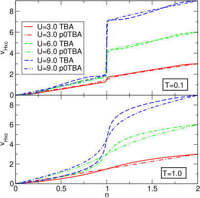
Figure 3: Comparison of the fully numerical TBA Hxc potential with p0TBA parametrization of Eq. (27) for different interactions and two typical temperatures.

We use these observations to design a hierarchy of analytic parametrizations of the fully numerical TBA Hxc potential which can easily be used in practical calculations. In the construction of these parametrization we make use of the simple analytic form of the Hxc potential of the single site model discussed in Sec. II.2.

IV.1 Lowest level single-site-motivated parametrization of the numerical TBA: p0TBA

Our simplest functional is aimed at reproducing the main qualitative features of the full numerical TBA based Hxc potential. These are the point symmetry of the function $v_{\rm Hxc}^{\rm TBA}(n)$ (reflecting the electron-hole symmetry), and the step structure at $n=1$, which gradually washes out at higher temperatures.

Precisely this pattern is also observed in the Hxc potential of the single-site model: in the zero-temperature limit, the Hxc potential $v_{\rm Hxc}^{\rm SSM}(n)$ has a step of height $U$. This almost discontinuous feature at low temperatures crosses over to a smooth one at high temperatures. Hence we will use the analytic form of $v_{\rm Hxc}^{\rm SSM}$ to mimic the step feature in our “lowest level” parametrization of the TBA Hxc potential. We adopt the simplest possible way to reproduce the correct low temperature amplitude of the step. Namely, in the function $v_{\rm Hxc}^{\rm SSM}(n,U,T)$, defined in Eqs. (16)-(17), the parameter $U$ will be replaced by the zero-temperature Mott-Hubbard gap $\Delta_{0}(U)$ of Eq. (26). The reduction of the gap automatically reduces the value of the potential at $n=2$ from the exact value of $U$ down to $\Delta_{0}(U)$. This unwanted behavior is corrected by adding a proper linear function that also ensures the right point symmetry of the Hxc potential. Putting all these arguments together we propose the following simple zero-level parametrization for the TBA Hxc potential (p0TBA)

$$v_{\rm Hxc}^{\rm p0TBA}(n)=\frac{U-\Delta_{0}(U)}{2}n+v_{\rm Hxc}^{\rm SSM}(n,\Delta_{0}(U),T).$$ (27)

The Hxc potential defined by this equation is shown in Fig. 3 together with the full numerical $v_{\rm Hxc}^{\rm TBA}(n)$. We clearly see that for all $T$ and $U$ the parametrization proposed in Eq. (27) overall agrees reasonably well with $v_{\rm Hxc}^{\rm TBA}(n)$. The maximal deviations never exceed unity (i.e., the value of the hopping integral $t$). Obviously the simple linear form of the first term of Eq. (27) is not flexible enough to reproduce the detailed features of the full TBA Hxc potential away from the step (see Fig. 3). However, as long as the difference between the parametrization and the full TBA Hxc potential are small compared to $t$, these inaccuracies are, in most practical cases, of little consequence for the solution of the KS equations, as will be confirmed in Sec. VI. It is also worth noting that a reasonably accurate practical approximation of Eq. (27) does not actually require the solution of the TBA equation. The only input we used was a zero-temperature Mott-Hubbard gap and general symmetry arguments. This observation can be useful to construct local approximations for more complicated, e. g. multidimensional, lattice models for which no exact solutions are available.

Apparently there are cases when the fine structure of the density distribution cannot fully be captured within our simplest zero-level parametrization p0TBA defined by Eq. (27). Therefore it is desirable to design a refined parametrization which further reduces the deviation from the numerical TBA potential. Two successive refinements of the “first-level” (p1TBA), and of the “second level” (p2TBA) are described in the next two subsections.

IV.2 First-level refined parametrization correcting the temperature dependence: p1TBA

Fig. 3 clearly shows that the temperature dependence of our simple p0TBA potential Eq. (27) is not perfect. At higher temperatures the step in the function $v_{\rm Hxc}^{\rm p0TBA}(n)$ washes out too fast as compared to the numerical $v_{\rm Hxc}^{\rm TBA}(n)$. There is an obvious physical reason for this deficiency. When the temperature $T$ increases and becomes larger than unity (in units of the hopping integral $t$), the kinetic energy contribution to the partition function becomes less and less important. Therefore at $T>1$, and independently of $U$, the system should behave more or less like a collection of independent sites with the Hxc potential given by the pure SSM expression of Eqs. (16)-(17).

In our first-level refinement (p1TBA) we take into account this physics by replacing $\Delta_{0}(U)$ in Eq. (27) with a “temperature-dependent gap” $\Delta_{1}(U,T)$

$$v_{\rm Hxc}^{\rm p1TBA}(n)=\frac{U-\Delta_{1}(U,T)}{2}n+v_{\rm Hxc}^{\rm SSM}(n,\Delta_{1}(U,T),T).$$ (28)

The function $\Delta_{1}(U,T)$ reduces to $\Delta_{0}(U)$ at $T\ll 1$ and approaches $U$ in the opposite limit of $T\gg 1$. The two limits are connected by a smooth function which is determined by comparison with the numerical TBA data. We have found that the following Padé-like form does the required job

$$\Delta_{1}(U,T)=\frac{\Delta_{0}(U)+a^{(1)}(T)T+UT^{2}}{1+T^{2}}$$ (29)

with

$$a^{(1)}(T)=\frac{a_{1}^{(1)}T+a_{2}^{(1)}}{T^{2}+a_{3}^{(1)}}\,.$$

Here $a_{1}^{(1)}=0.95,a_{2}^{(1)}=-0.08,a_{3}^{(1)}=0.13$.

From Fig. 4 we see that the first-level parametrization p1TBA, Eqs. (28)-(29), produces an Hxc potential which is practically indistinguishable from the full numerical $v_{\rm Hxc}^{\rm TBA}(n)$, provided that $T$ is not too small. However, there are still some deviations in the low-temperature regime. This point is addressed at the last step in our three-level hierarchy of parametrizations.

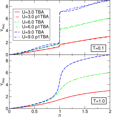
Figure 4: Comparison of the fully numerical TBA Hxc potential with the first-level refined p1TBA parametrization of Eq. (28) for two typical temperatures.

IV.3 Second-level refinement – the best analytic fit to numerical TBA: p2TBA

The only feature missing in the first-level p1TBA parametrization is a low-temperature nonlinearity of $v_{\rm Hxc}^{\rm TBA}(n)$ away from the half filling (see upper panel of Fig. 4). Physically the nonlinearity should be attributed to a nontrivial density of states in the Hubbard bands. According to our experience the remaining inaccuracy in the Hxc potential has practically no effect on the density distribution. On the other hand, we cannot exclude that in some situations (steep external potentials and/or small number of particles) the low-temperature inaccuracy of $v_{\rm Hxc}^{\rm p1TBA}(n)$ will produce visible (thought definitely not large) errors in the density. To avoid such problems we go to the last step in our hierarchy and introduce a nonlinear correction term. A very satisfactory fit to the numerical $v_{\rm Hxc}^{\rm TBA}(n)$ can be achieved with the following (p2TBA) form

$$v_{\rm Hxc}^{\rm p2TBA}(n)=\frac{U-\Delta_{2}(U,T)}{2}n+v_{\rm Hxc}^{\rm SSM}(n,\Delta_{2}(U,T),T)$$ (30)

$$-A(U,T)\sin[2\pi(n-1)]-B(U,T)\sin[\pi(n-1)].$$

We note that the analytic form of the correction term in Eq. (30) automatically preserves the point symmetry of the potential and the exact values at the end points, $n=0$ and $n=2$. Note also that we use a new function $\Delta_{2}(U,T)$ defined by

$$\Delta_{2}(U,T)=\frac{\Delta_{0}(U)+a^{(2)}(T)T+UT^{2}}{1+T^{2}}$$ (31)

with

$$a^{(2)}(T)=\frac{a_{1}^{(2)}T+a_{2}^{(2)}}{T+a_{3}^{(2)}}$$

and the coefficients are $a_{1}^{(2)}=-0.28$, $a_{2}^{(2)}=2.2$, and $a_{3}^{(2)}=0.50$. As before, in the zero-temperature limit $\Delta_{2}(U,T)$ reduces to the correct zero-temperature gap $\Delta_{0}(U)$ while in the high-temperature limit it becomes $U$. The interaction and temperature dependent coefficients $A(U,T)$ and $B(U,T)$ in Eq. (30) are parametrized as follows

$$A(U,T)=\frac{A_{1}(T)U^{2}}{U^{2}+A_{2}(T)},\,B(U,T)=\frac{B_{1}(T)U^{2}}{U^{2}+B_{2}(T)}\,,$$ (32)

with

$$A_{1}(T)=\frac{A_{11}}{T^{2}+A_{12}},\,A_{2}(T)=\frac{A_{21}}{T^{2}+A_{22}}\,,$$ (33)

$$B_{1}(T)=\frac{B_{11}}{T^{2}+B_{12}},\,B_{2}(T)=\frac{B_{21}}{T^{2}+B_{22}}\,.$$ (34)

Here $A_{11}=0.09,A_{12}=0.25,A_{21}=705.5,A_{22}=24.95$ and $B_{11}=0.05,B_{12}=0.13,B_{21}=0.65,B_{22}=0.01$. The accuracy of this parametrization can be appreciated in Fig. 5: at the scale of the plot, the parametrization p2TBA and the full numerical TBA Hxc potentials are essentially indistinguishable.

Our parametrization of the finite-temperature TBA results generalizes earlier parametrizations LimaSilvaOliveiraCapelle:03 ; FrancaVieiraCapelle:12 valid for zero temperature. Close comparison of the Hxc potential of our p2TBA parametrization of Eq. (30) in the zero-temperature limit with the FVC parametrization of Ref. FrancaVieiraCapelle:12, and exact zero-temperature results reveals that the p2TBA parametrization in some density ranges can be marginally less accurate than FVC. As pointed out before, however, in contrast to FVC our parametrization by construction incorporates the exact zero-temperature gap. Since the most prominent feature of the Hxc potential as function of density is precisely the discontinuity at half-filling, i.e., the zero-temperature gap, in some situations the incorrect gap of FVC might lead to spurious features as will be shown below.

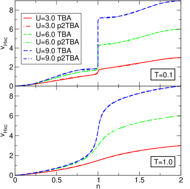
Figure 5: Comparison of the fully numerical TBA Hxc potential with the second-level refined p2TBA parametrization of Eq. (30) for two typical temperatures.

V Self-consistency with rapidly varying functionals using bisection

In the previous Section we presented a hierarchy of explicit local approximations for the Hxc potential of lattice DFT, which at low temperatures are rapidly varying functions of the density close to half-filling. In Sec. II we have pointed out the difficulties in converging the usual self-consistency cycle for solving the KS equation (1) with such functionals. In the present Section we show how to avoid the convergence problem and present a numerically feasible algorithm to obtain the self-consistent solution based on bisection techniques.

We begin by writing again the self-consistency equation for the density at site $i$, Eq. (24), in a form of a fixed point problem, i. e., making explicit its dependence on the densities at all other sites:

$$n_{i}=\sum_{\alpha}f(\varepsilon_{\alpha}({\bf n}))|\varphi^{(\alpha)}_{i}({\bf n})|^{2}\equiv G_{i}[{\bf n}]$$ (35)

where

$${\bf n}=(n_{1},n_{2},\ldots,n_{N_{s}})$$ (36)

and the orbitals are calculated from the KS equation (23) using the KS potential

$$v_{i}^{\rm KS}(n_{i})=v_{i}+v_{\rm Hxc}^{\rm mod}(n_{i})\;.$$ (37)

The set of equations (35) for $i\in{1,\ldots,N_{s}}$ constitute a coupled set of $N_{s}$ nonlinear equations for the $N_{s}$ ground-state densities $n_{i}$, $i=1,\ldots,N_{s}$. As we have argued in Sec. II, the numerical solution of these equations by plain iterations produces a non-converging sequence. Obviously more elaborate iterative schemes, such as the Newton-Rhapson method, which incorporates information on derivatives of the equations with respect to the unknown variables are also not appropriate because those derivatives may become very large (in the low-temperature regime). This again leads to convergence problems in the iterative solution of the coupled nonlinear equations.

Here we propose a solution scheme based on bisection. The main idea of our algorithm is inspired by the exactly solvable single-site KS problem described in Sec. II.2. Therefore we first explain it for this simple, but very illuminating case. Instead of iteratively searching for the fixed point of function $G(n)$ in Eq. (18) we rewrite this equation as

$$n-G(n)=0,$$ (38)

and search for zeros of the left hand side. From the uniqueness of the solution we know that there is only one zero, and, by construction, the l.h.s. of Eq. (38) has different signs at the end points, $n=0$ and $n=2$, of the density interval. Therefore the standard bisection method PressTeukolskyVetterlingFlannery:86 is applicable. Starting from the end points and using bisections we can bracket the solution to any desired accuracy.

For the general lattice KS problem we need to solve a system of Eqs. (35). In this case the following straighforward multidimensional generalization of the standard bisection method can be used. We start with an initial guess $n_{i}^{(0)}$ for the densities at sites $i\in\{2,\ldots,N_{s}\}$. We then define the density vector

$${\bf n}^{(1)}=\left(n_{1},n_{2}^{(0)},\ldots,n_{N_{s}}^{(0)}\right)\;,$$ (39)

insert this density vector in the rhs of Eq. (35) for $i=1$ and solve the resulting nonlinear equation for the density $n_{1}=n_{1}^{(1)}$ with the usual 1D bisection method. Then we choose the density vector

$${\bf n}^{(2)}=\left(n_{1}^{(1)},n_{2},n_{3}^{(0)},\ldots,n_{N_{s}}^{(0)}\right)\;,$$ (40)

insert it into Eq. (35) for $i=2$ and solve for $n_{2}=n_{2}^{(1)}$ again by bisection. In the next step we take

$${\bf n}^{(3)}=\left(n_{1}^{(1)},n_{2}^{(1)},n_{3},n_{4}^{(0)},\ldots,n_{N_{s}}^{(0)}\right)$$ (41)

and solve Eq. (35) for $i=3$ for $n_{3}=n_{3}^{(0)}$. We continue the procedure until we have exhausted the $N_{s}$ equations (35). Then we start the cycle all over but now with the initial guess for the density ${\bf n}^{(N_{s}+1)}$ as Eq. (39) but with the $n_{i}^{(0)}$ replaced by $n_{i}^{(1)}$. The whole process is continued until convergence is achieved.

In Fig. 6 we illustrate the iterative procedure for a symmetric three-site problem, i.e., for $v_{1}=v_{3}$ and by symmetry also $v_{1}^{\rm KS}=v_{3}^{\rm KS}$. We then need to solve two coupled nonlinear equations of the form

$$n_{1} - G_{1}(n_{1},n_{2})=0,$$ (42)

$$n_{2} - G_{2}(n_{1},n_{2})=0.$$ (43)

In Fig. 6 we show the $(n_{1},n_{2})$ plane and zero lines for the l.h.s. of Eqs. (42) and (43). The overall solution of the problem is given by the intersection of these two lines. Furthermore, the dashed line in Fig. 6 shows how our iterative scheme converges to this solution.

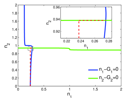
Figure 6: Solution lines of $n_{i}-G_{i}(n_{1},n_{2})=0$, $i=1,2$, for the symmetric three-site problem. The intersection of these two lines is the solution to the system of Eqs. (42)-(43). The parameters are $U=8$, $\mu=0.5$, $v_{1}=2$, $v_{2}=0$, and $T=0.5$.

From this example we can also understand that in some cases the proposed scheme, as is, may not converge. If the zero lines close to the intersection become just straight lines then, depending on the slopes of these lines, the iterative scheme may follow a rectangular path encircling the solution point but never reaching it. However, in this case one additional Newton-Rhapson step (using information on the derivatives) will directly lead to the solution point.

As is common in DFT, we have used the densities as fundamental variables in Eq. (35). It is also possible to implement the bisection scheme in terms of the KS potentials. To this end we write the vector of Hxc potentials at sites $i$ as

$${\bf v}_{\rm Hxc}=\left(v_{{\rm Hxc},1},\ldots,v_{{\rm Hxc},N_{s}}\right)$$ (44)

and consider both the KS orbitals and eigenvalues as functions of this vector, i.e., $\varphi^{(\alpha)}=\varphi^{(\alpha)}({\bf v}_{\rm Hxc})$ and $\varepsilon^{(\alpha)}=\varepsilon^{(\alpha)}({\bf v}_{\rm Hxc})$. Therefore, also the density at site $i$ can be considered a function of ${\bf v}_{\rm Hxc}$ through

$$n_{i}({\bf v}_{\rm Hxc})=\sum_{\alpha}f(\varepsilon_{\alpha}({\bf v}_{\rm Hxc}))|\varphi^{(\alpha)}_{i}({\bf v}_{\rm Hxc})|^{2}\;.$$ (45)

For our local approximations to the Hxc potentials the set of nonlinear equations to be solved by bisection then becomes

$$v_{{\rm Hxc},i}=v_{\rm Hxc}^{\rm mod}(n_{i}({\bf v}_{\rm Hxc}))$$ (46)

with the local density $n_{i}({\bf v}_{\rm Hxc})$ given by Eq. (45). In order to solve this set of equations we proceed in an analogous way to the one described above for the density-based procedure but now treating the local Hxc potentials $v_{{\rm Hxc},i}$ at site $i$ as the unknowns to be determined.

VI Numerical applications

In this Section we present some numerical examples demonstrating successful applications of our self-consistency algorithm as well as the accuracy of the local approximation using our different parametrizations.

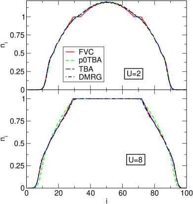
Figure 7: Density distribution of $N=70$ particles in the harmonic potential at $T=0$ (upper panel: $U=2$, lower panel: $U=8$). The strength of the external potential is $V_{\rm ext}=2.5\times 10^{-3}$. We compare the exact DMRG results against DFT results based on different choices for $v_{\rm Hxc}$. They are the parametrization of Ref. FrancaVieiraCapelle:12, (labeled as FVC), our lowest-level parametrization p0TBA of Eq. (27) (labeled as p0TBA), and the full numerical TBA potential (labeled as TBA), respectively. The results obtained with the p2TBA potential of Eq. (30) are indistinguishable from the full TBA results.

We illustrate our theoretical developments by calculating the density distribution of particles confined by an external harmonic potential of the form

$$v_{i}=V_{\rm ext}\;(i-i_{0})^{2}$$ (47)

where $V_{\rm ext}$ is the strength of the trapping potential and $i_{0}=(N_{s}+1)/2$ (we take $V_{\rm ext}$ in units of the hopping parameter $t$). The Hubbard chain with a superimposed harmonic potential is commonly used to model the behavior of cold fermionic gases in 1D optical lattices  RigolMuramatsuBatrouniScalettar:03 ; LiuDrummondHu:05 ; CampoCapelle:05 ; XianlongPoliniTanatarTosi:06 ; Heiselberg:06 ; YamamotoYamadaOkumuraMachida:11 . Therefore our results below have a clear relevance for the physics of cold trapped atoms. However, for our present illustrative purposes, the choice of this particular system is related to one of its specific features, namely the possible coexistence of the Mott insulator phase around the center of the trap and the metallic phase at the trap’s edges RigolMuramatsuBatrouniScalettar:03 ; LiuDrummondHu:05 ; XianlongPoliniTosiCampoCapelleRigol:06 . In the Mott phase the density is pinned at $n=1$ which shows up as an extended plateau in the density distribution. Therefore in trapped systems the appearance of the Mott insulator phase becomes detectable within the “density-only“ DFT concept. On the other hand, at the level of DFT functionals the Mott physics is solely related to the discontinuity of the xc potential. Thus the Hubbard model with a harmonic confinement is perfectly suited for demonstrating the working power of our algorithm as well as the performance of different parametrizations for the Hxc potentials.

As a first example we study a system with $N=70$ particles on $N_{s}=100$ sites in the presence of the potential given by Eq. (47) with $V_{\rm ext}=2.5\times 10^{-3}$. In Fig. 7 we show self-consistent densities for two different values of the Hubbard interaction, $U=2$ and $U=8$, evaluated at zero temperature. Except for the DMRG results which denotes numerically exact reference results from density matrix renormalization group calculations White:92 ; Schollwoeck:05 ; Albuquerque:07 , all other calculations result from self-consistent DFT calculations with local approximations to the Hxc potential. FVC denotes the zero-temperature BALDA using the parametrization of Ref. FrancaVieiraCapelle:12, , p0TBA denotes results obtained with our low-level parametrization of Eq. (27), the results obtained from our second-level parametrization of Eq. (30) are indistinguishable from those using the exact numerical TBA as input in the local approximation.

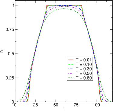
Figure 8: Melting of the Mott phase at finite temperature. The calculations are based on the p2TBA parametrization which produces the results identical to those of the full numerical TBA. The parameters are $U=8$, $V_{\rm ext}=2.5\times 10^{-3}$, $N=70$.

We see that the density profiles are quite similar in the different approaches. For $U=2$ the FVC parametrization exhibits two spurious density plateaus around $i\approx 30$ and $i\approx 70$ which are due to the fact that this parametrization does not incorporate the zero-temperature derivative discontinuity exactly but only approximately. We also see some small differences between the p0TBA and the TBA results in the flanks of the density profile. For stronger interaction, $U=8$, the density exhibits an extended plateau of value unity over a wide range of sites in the center of the well which physically corresponds to the local, incompressible Mott phase. On the other hand, in the density functional picture this plateau is a direct consequence of the extremely rapid variation of the Hxc potentials as function of the density. The small difference in the p0TBA and TBA densities is related to the nonlinearity of Hxc potential away from the half filling (see Sec. IV.3). This deficiency is corrected in our second level parametrization p2TBA of Eq. (30). As a result the density calculated with the p2TBA Hxc potential is completely indistinguishable from that obtained using the full numerical TBA potential. This also holds true for all interactions, temperatures and trapping potentials we have tried. Hence in practice in all figures the results denoted as TBA have been actually produced using the p2TBA potential defined after Eq. (30). At strictly zero temperature, the KS potential has a real discontinuity at integer filling $n=1$ and, therefore, it is undefined in this point. For practically solving Eqs. (35)-(37) in this case we replace the discontinuity by a linear function when $n\in[1-\Delta n,1+\Delta n]$ with $\Delta n=10^{-3}$. Further decreasing $\Delta n$ will not hamper the convergency and the final results. In general, the densities from the DFT calculations are remarkably close to the numerically exact quantum Monte-carlo/DMRG result RigolMuramatsuBatrouniScalettar:03 ; XianlongPoliniTosiCampoCapelleRigol:06 ; HuWangXianlongOkumuraIgarashiYamadaMachida:10 .

Unlike earlier work LimaSilvaOliveiraCapelle:03 ; FrancaVieiraCapelle:12 , our parametrization is valid for arbitrary temperature and thus allows to study finite temperature effects. As a first application of this feature, in Fig. 8 we show how the density plateau due to the local Mott phase “melts away” when increasing the temperature.

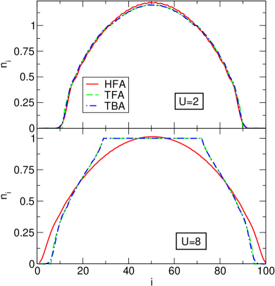
Figure 9: Comparison of the density distributions at $T=0$ obtained using Hartree-Fock approximation (HFA), Thomas-Fermi approximation (TFA) against DFT results based on the TBA potential (TBA). The parameters are the same as in Fig. 7.

We have also calculated (Fig. 9) the density profiles at zero temperature in the Hartree-Fock (HFA) and Thomas-Fermi approximation (TFA). Here, by TFA we mean that the non-interacting kinetic energy is not treated exactly as in the Kohn-Sham scheme but at the level of a local approximation. It is important to note, however, that exchange-correlation effects are also included at the level of the local density approximation (in Ref. XianlongPoliniTosiCampoCapelleRigol:06, this approximation has been denoted as “total-energy LDA (TLDA)”). The top panel of Fig. 9 shows that for small values of $U$ both the HFA and the TFA give a reasonably accurate density profile when compared to DMRG. For larger values of $U$ ($U=8$, lower panel of Fig. 9), however, the situation is different: HFA completely misses the development of the density plateau while TFA (due to the local Hxc potential) does exhibit this plateau. Moreover, in HFA the density is more spread out as compared to the exact result.

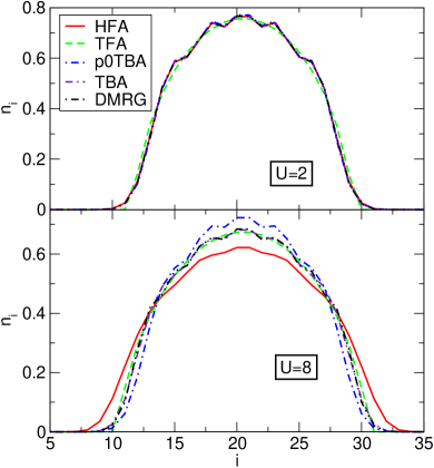
Figure 10: Density distribution of $N=10$ particles in a harmonic trap at temperature $T=0$ in Hartree-Fock (HFA) and Thomas-Fermi approximations (TFA), compared to DFT results based on TBA and DMRG. Upper panel: $U=2$, lower panel: $U=8$. The external potential is $V_{\rm ext}=2.5\times 10^{-2}$.

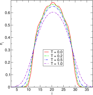
Figure 11: Effects of finite temperatures on the density profile of $N=10$ particles in a harmonic trap. The calculation is based on the full numerical TBA. The parameters are $U=8$, $V_{\rm ext}=2.5\times 10^{-2}$.

The differences between TFA and both the DMRG as well as the full KS results with the TBA functional are more pronounced for smaller number of particles. In Fig. 10 we show the density profile for $N=10$ electrons on $N_{s}=40$ sites in the harmonic external potential of Eq. (47) with $V_{\rm ext}=2.5\times 10^{-2}$. Not surprisingly, the TFA approximation completely misses the quantum oscillations in the density profile both for small and large values of $U$. In contrast, HFA captures these oscillations well for small $U$ since the kinetic energy is treated at a quantum level. In contrast, for $U=8$ the correlation effects are too strong to be captured by HFA which, again, shows a density distribution which is too spread out. On the other hand, the KS calculation using the TBA again is in extremely good agreement with the DMRG results. The lower panel of Fig. 10 also shows that for this case our simplest p0TBA parametrization of the TBA results can sometimes lead to inaccuracies. Finally, in Fig. 11, solving the KS equations with the TBA functional, we show the effect of temperature on the density profile: one can see that the quantum oscillations due to the relatively small number of particles seen for zero temperature are quickly suppressed when increasing the temperature.

VII Conclusions

In this work we have suggested a way to deal with convergence problems in self-consistent KS calculations when dealing with (local) approximations for the xc potential which exhibit rapid variations as function of the density. Working in the framework of lattice DFT, we have formulated the KS self-consistency cycle as a fixed point problem and shown that for rapidly varying functionals the fixed point in the usual prcedure is not attractive. Instead, we rephrased the search for the self-consistent KS potential in terms of finding the roots of a set of coupled nonlinear equations. To find these solutions, we then suggested an iterative algorithm based on successive application of the well-known bisection method for finding roots of nonlinear equations in one dimension. The scheme has been successfully tested for model systems of electrons in a harmonic trap interacting via a Hubbard interaction. We have used a newly designed local approximation for the xc functional based on the thermodynamic Bethe ansatz solution of the uniform Hubbard model. Based on these results we constructed simple, yet accurate parametrizations for arbitrary temperatures, thus generalizing earlier parametrizations suggested for zero temperature. This paves the way for further investigations on the performance of finite-temperature DFT for one-dimensional lattice models.

*

Appendix A Hartree-exchange-correlation free energy per site for the TBA parametrizations

In Sec. IV we have suggested a local density approximation for one-dimensional lattice systems based on the numerical solution of the TBA for the uniform Hubbard model. The parametrizations we proposed were constructed from insights gained on the numerical results for the Hxc potential. However, typically the construction of local DFT approximations starts by modelling the xc energy per site and the corresponding xc potential is then obtained by differentiation. In this Appendix we derive the expressions for the Hxc free energies per site for the different parametrizations suggested in Sec. IV.

We start with the derivation of the exact LDA Hxc free energy per site at finite temperature, expressed in terms of general thermodynamic quantities. As usual, a crucial ingredient of the general construction of LDA is a reference system of interacting particles with uniform density for which the grand canonical potential per site, $\Omega(\mu)$, is written as function of the chemical potential $\mu$. The partition function for the reference system is

$$Z(\mu)=\exp(-\beta\Omega(\mu))$$ (48)

from which we can derive the density as function of $\mu$,

$$n(\mu)=-\frac{\partial\Omega(\mu)}{\partial\mu}=\frac{1}{\beta}\frac{\partial\ln Z(\mu)}{\partial\mu}\;.$$ (49)

This function can be inverted to give the chemical potential as function of density, $\mu=\mu(n)$. By Legendre transformation we can then obtain the free energy per site of the reference system as function of density as

$$F(n)=\Omega(\mu(n))+\mu(n)n\;.$$ (50)

We can repeat the same steps for the corresponding non-interacting reference with the same uniform density $n$ with grand canonical potential per site $\Omega_{s}(\mu_{s})$ and the corresponding expression for the free energy per site

$$F_{s}(n)=\Omega_{s}(\mu_{s}(n))+\mu_{s}(n)n\;.$$ (51)

The Hxc free energy per site is then simply given by

$$F_{\rm Hxc}(n)=F(n)-F_{s}(n)$$ (52)

$$= -\frac{1}{\beta}\ln\left(\frac{Z(\mu_{s}(n)+v_{\rm Hxc}(n))}{Z_{s}(\mu_{s}(n))}\right)+nv_{\rm Hxc}(n)$$

where we have defined the Hxc potential as

$$v_{\rm Hxc}(n)=\mu(n)-\mu_{s}(n)$$ (53)

(see also Eq. (25)).

Applying Eq. (52) to the single-site model of Section II.2, we obtain for the Hxc free energy per site of that model

$$F_{\rm Hxc}^{\rm SSM}(n,U,T)=nv_{\rm Hxc}^{\rm SSM}(n,U,T)$$ (54)

$$-\frac{1}{\beta}\ln\left(\frac{Z^{\rm SSM}(\mu_{s}^{\rm SSM}(n,T)+v_{\rm Hxc}^{\rm SSM}(n,U,T))}{Z_{s}^{\rm SSM}(\mu_{s}^{\rm SSM}(n,T))}\right)$$

where the Hxc potential of the SSM model, $v_{\rm Hxc}^{\rm SSM}(n,U,T))$, is given by Eq. (16) and we have made explicit the dependence on the temperature $T$ and the on-site interaction $U$. It remains to find the dependence of $Z^{\rm SSM}$ and $Z_{s}^{\rm SSM}$ on the density. This can be done by performing the program described above with the interacting and non-interacting partition functions of the SSM model given in Eqs. (11) and (14). Actually, we have already calculated the dependence of the chemical potential on the density (see Eq. (15))

$$\mu_{s}^{\rm SSM}(n,T)=-\tilde{v}_{s}(n)=\frac{1}{\beta}\ln\left(\frac{n}{2-n}\right)$$ (55)

which, when inserted back into Eq. (14), yields the non-interacting partition function of the SSM model in terms of the density

$$Z_{s}^{\rm SSM}(n)=\left(\frac{2}{2-n}\right)^{2}\;.$$ (56)

Finally, the interacting partition function of the SSM model (see Eq. (11)) may be written in terms of the density as

$$Z^{\rm SSM}(n,U,T)=1+\frac{2n}{2-n}\exp\left(\beta v_{\rm Hxc}^{\rm SSM}(n,U,T)\right)$$ (57)

$$+\frac{n^{2}}{(2-n)^{2}}\exp\left(\beta(2v_{\rm Hxc}^{\rm SSM}(n,U,T)-U)\right)$$

which leads to the final result for the Hxc free energy per site of the SSM model

$$F_{\rm Hxc}^{\rm SSM}(n,U,T)=nv_{\rm Hxc}^{\rm SSM}(n,U,T)$$ (58)

$$-\frac{1}{\beta}\ln\Bigg{[}\left(1-\frac{n}{2}\right)^{2}+n\left(1-\frac{n}{2}\right)\exp\left(\beta v_{\rm Hxc}^{\rm SSM}(n,U,T)\right)$$

$$\;\;\;\;\;\;\;\;\;\;\;\;\;\;\;+\frac{n^{2}}{4}\exp\left(\beta(2v_{\rm Hxc}^{\rm SSM}(n,U,T)-U)\right)\Bigg{]}\;.$$

By construction, the derivative of this expression with respect to the density yields the SSM Hxc potential of Eq. (16).

Using this result it is now easy to express the Hxc free energies per site for our different parametrizations of the TBA results. For the lowest-level parametrization (p0TBA) of the TBA the resulting expression reads

$$F_{\rm Hxc}^{\rm p0TBA}(n,U,T)=\frac{U-\Delta_{0}(U)}{4}n^{2}+F_{\rm Hxc}^{\rm SSM}(n,\Delta_{0}(U),T)$$ (59)

where $\Delta_{0}(u)$ is the exact zero-temperature gap of the uniform Hubbard model given by Eq. (26). For the first-level refinement (p1TBA), it has the same form except that $\Delta_{0}(U)$ is replaced by $\Delta_{1}(U,T)$ of Eq. (29), i.e.,

$$F_{\rm Hxc}^{\rm p1TBA}(n,U,T) = \frac{U-\Delta_{1}(U,T)}{4}n^{2}$$ (60)

$$+F_{\rm Hxc}^{\rm SSM}(n,\Delta_{1}(U,T),T)\;.$$

Finally, for the second refined parametrization (p2TBA) we have

$$F_{\rm Hxc}^{\rm p2TBA}(n,U,T)=\frac{U-\Delta_{2}(U,T)}{4}n^{2}$$ (61)

$$+F_{\rm Hxc}^{\rm SSM}(n,\Delta_{2}(U,T),T)+\frac{A(U,T)}{2\pi}\left(\cos(2\pi(n-1))-1\right)$$

$$+\frac{B(U,T)}{\pi}\left(\cos(\pi(n-1))+1\right)$$

with $\Delta_{2}(U,T)$ given by Eq. (31) and the functions $A(U,T)$ and $B(U,T)$ given by Eq. (32).

It is worth mentioning that for zero temperature, since $\Delta_{2}(U,0)=\Delta_{1}(U,0)=\Delta_{0}(U)$, the contributions to the Hxc free energy per site coming from the single-site model in all our parametrizations (59)-(61) reduce to the same limit

$$F_{\rm Hxc}^{\rm SSM}(n,\Delta_{0}(U),0)=\Delta_{0}(U)(n-1)\Theta(n-1)$$ (62)

where $\Theta(x)$ is the Heaviside step function.

References

- (1) P. Hohenberg and W. Kohn, Phys. Rev. 136, B864 (1964).
- (2) W. Kohn and L.J. Sham, Phys. Rev. 140, A1133 (1965).
- (3) O. Gunnarsson and K. Schönhammer, Phys. Rev. Lett. 56, 1968 (1986).
- (4) N.A. Lima, M.F. Silva, L.N. Oliveira, and K. Capelle, Phys. Rev. Lett. 90, 146402 (2003).
- (5) G. Xianlong, M. Polini, M.P. Tosi, V.L. Campo, K. Capelle, and M. Rigol, Phys. Rev. B 73, 165120 (2006).
- (6) P.N. Ma, S. Pilati, M. Troyer, and X. Dai, Nat. Phys. 8, 601 (2012).
- (7) D. Jaksch and P. Zoller, Ann. Phys. 315, 52 (2005); M. Lewenstein, A. Sanpera, V. Ahufinger, B. Damski, A. Sen(De), and U. Sen, Adv. Phys. 56, 243 (2007); I. Bloch, J. Dalibard, and W. Zwerger, Rev. Mod. Phys. 80, 885 (2008).
- (8) K. Schönhammer, O. Gunnarsson, and R.M. Noack, Phys. Rev. B 52, 2504 (1995).
- (9) M.F. Silva, N.A. Lima, A.L. Malvezzi, and K. Capelle, Phys. Rev. B 71, 125130 (2005).
- (10) M. Ijäs and A. Harju, Phys. Rev. B 82, 235111 (2010).
- (11) D. Karlsson, A. Privitera, and C. Verdozzi, Phys. Rev. Lett. 106, 116401 (2011).
- (12) N.A. Lima, L.N. Oliveira, and K. Capelle, Europhys. Lett. 60, 601 (2002).
- (13) J.P. Perdew, R.G. Parr, M. Levy, and J.L. Balduz, Phys. Rev. Lett. 49, 1691 (1982).
- (14) G. Xianlong, M. Rizzi, M. Polini, R. Fazio, M.P. Tosi, V.L. Campo, and K. Capelle, Phys. Rev. Lett. 98, 030404 (2007).
- (15) S. Schenk, M. Dzierzawa, P. Schwab, and U. Eckern, Phys. Rev. B 78, 165102 (2008).
- (16) A. Akande and S. Sanvito, Phys. Rev. B 82, 245114 (2010).
- (17) A. Akande and S. Sanvito, J. Phys. Condens. Matter 24, 055602 (2012).
- (18) C. Verdozzi, Phys. Rev. Lett. 101, 166401 (2008); W. Li, G. Xianlong, C. Kollath, and M. Polini, Phys. Rev. B 78, 195109 (2008).
- (19) D. Karlsson, C. Verdozzi, M.M. Odashima, and K. Capelle, Europhys. Lett. 93, 23003 (2011).
- (20) S. Kurth, G. Stefanucci, E. Khosravi, C. Verdozzi, and E.K.U. Gross, Phys. Rev. Lett. 104, 236801 (2010).
- (21) N. Mermin, Phys. Rev. 137, A1441 (1965).
- (22) G. Stefanucci and S. Kurth, Phys. Rev. Lett. 107, 216401 (2011).
- (23) F. Evers and P. Schmitteckert, Phys. Chem. Chem. Phys. 13, 14417 (2011).
- (24) E.H. Lieb and F.Y. Wu, Phys. Rev. Lett 20, 1445 (1968).
- (25) M. Takahashi, Prog. Theor. Phys. 47, 69 (1972).
- (26) N. Kawakami, T. Usuki, and A. Okiji, Phys. Lett. A 137, 287 (1989).
- (27) T. Usuki, N. Kawakami, and A. Okiji, J. Phys. Soc. Jpn 59, 1357 (1990).
- (28) M. Takahashi and M. Shiroishi, Phys. Rev. B 65, 165104 (2002).
- (29) W.H. Press, S.A. Teukolsky, W.T. Vetterling, and B.P. Flannery, Numerical Recipes: The Art of Scientific Computing (Cambridge University Press, New York, 1986).
- (30) V.V. França, D. Vieira, and K. Capelle, New J. Phys. 14, 073021 (2012).
- (31) M. Rigol, A. Muramatsu, G.G. Batrouni, and R.T. Scalettar, Phys. Rev. Lett. 91, 130403 (2003).
- (32) X.-J. Liu, P.D. Drummond, and H. Hu, Phys. Rev. Lett. 94, 136406 (2005).
- (33) V.L. Campo and K. Capelle, Phys. Rev. A 72, 061602(R) (2005).
- (34) G. Xianlong, M. Polini, B. Tanatar, and M.P. Tosi, Phys. Rev. B 73, 161103(R) (2006).
- (35) H. Heiselberg, Phys. Rev. A 74, 033608 (2006).
- (36) A. Yamamoto, S. Yamada, M. Okumura, and M. Machida, Phys. Rev. A 84, 043642 (2011).
- (37) S.R. White, Phys. Rev. Lett. 69, 2863 (1992).
- (38) U. Schollwöck, Rev. Mod. Phys. 77, 259 (2005).
- (39) A.F. Albuquerque et al., J. Magn. Magn. Mater. 310, 1187 (2007).
- (40) J.-H. Hu, J.-J. Wang, G. Xianlong, M. Okumura, R. Igarashi, S. Yamada, and M. Machida, Phys. Rev. B 82, 014202 (2010).