Deterministic Team Problems with Signaling Incentive

Abstract

This paper considers linear quadratic team decision problems where the players in the team affect each other’s information structure through their decisions. Whereas the stochastic version of the problem is well known to be complex with nonlinear optimal solutions that are hard to find, the deterministic counterpart is shown to be tractable. We show that under a mild assumption, where the weighting matrix on the controller is chosen large enough, linear decisions are optimal and can be found efficiently by solving a semi-definite program.

Notation

$\mathbb{S}^{n}$	The set of $n\times n$ symmetric matrices.
$\mathbb{S}^{n}_{+}$	The set of $n\times n$ symmetric positive
	semidefinite matrices.
$\mathbb{S}^{n}_{++}$	The set of $n\times n$ symmetric positive
	definite matrices.
$\mathcal{C}$	The set of functions $\mu:\mathbb{R}^{p}\rightarrow\mathbb{R}^{m}$ with
	$\mu(y)=(\mu_{1}(y_{1}),\mu_{2}(y_{2}),...,\mu_{N}(y_{N}))$,
	$\mu_{i}:\mathbb{R}^{p_{i}}\rightarrow\mathbb{R}^{m_{i}}$, $\sum_{i}m_{i}=m$, $\sum_{i}p_{i}=p$.
$\mathbb{K}$	$\{K\in\mathbb{R}^{m\times p}|K=\oplus\sum K_{i},K_{i}\in\mathbb{R}^{m_{i}\times p_{i}}\}$
$A^{\dagger}$	Denotes the pseudo-inverse of the
	square matrix $A$.
$A_{\perp}$	Denotes the matrix with minimal number
	of columns spanning the nullspace of $A$.
$A_{i}$	The $i$th block row of the matrix $A$.
$A_{ij}$	The block element of $A$ in position$(i,j)$.
$\succeq$	$A\succeq B$ $\Longleftrightarrow$ $A-B\in\mathbb{S}^{n}_{+}$.
$\succ$	$A\succ B$ $\Longleftrightarrow$ $A-B\in\mathbb{S}^{n}_{++}$.
$\mathbf{Tr}$	$\mathbf{Tr}[A]$ is the trace of the matrix $A$.
$\mathcal{N}(m,X)$	The set of Gaussian variables with
	mean $m$ and covariance $X$.

I Introduction

The team problem is an optimization problem, where a number of decision makers (or players) make up a team, optimizing a common cost function with respect to some uncertainty representing nature. Each member of the team has limited information about the global state of nature. Furthermore, the team members could have different pieces of information, which makes the problem different from the one considered in classical optimization, where there is only one decision function that has access to the entire information available about the state of nature.

Team problems seemed to possess certain properties that were considerably different from standard optimization, even for specific problem structures such as the optimization of a quadratic cost in the state of nature and the decisions of the team members. In stochastic linear quadratic decision theory, it was believed for a while that certainty-equvalence holds between estimation and optimal decision with complete information, even for team problems. The certainty-equivalence principle can be briefly explained as follows. First assume that every team member has access to the information about the entire state of nature, and find the corresponding optimal decision for each member. Then, each member makes an estimate of the state of nature, which is in turn combined with the optimal decision obtained from the full information assumption. It turns out that this strategy does not yield an optimal solution (see [9]).

A general solution to static stochastic quadratic team problems was presented by Radner [9]. Radner’s result gave hope that some related problems of dynamic nature could be solved using similar arguments. But in 1968, Witsenhausen [11] showed in his well known paper that finding the optimal decision can be complex if the decision makers affect each other’s information. Witsenhausen considered a dynamic decision problem over two time steps to illustrate that difficulty. The dynamic problem can actually be written as a static team problem:

minimize $$\mathbf{E}\hskip 2.84526pt\left\{k_{0}u_{0}^{2}+(x+u_{0}-u_{1})^{2}\right\}$$

subject to $$u_{0}=\mu_{0}(x),\hskip 5.69054ptu_{1}=\mu_{1}(x+u_{0}+w),$$

where $x$ and $w$ are Gaussian with zero mean and variance $X$ and $W$, respectively. Here, we have two decision makers, one corresponding to $u_{0}$, and the other to $u_{1}$. Witsenhausen showed that the optimal decisions $\mu_{0}$ and $\mu_{1}$ are not linear because of the signaling/coding incentive of $u_{0}$. Decision maker $u_{1}$ measures $x+u_{0}+w$, and hence, its measurement is affected by $u_{0}$. Decision maker $u_{0}$ tries to encode information about $x$ in its decision, which makes the optimal strategy complex.

The problem above is actually an information theoretic problem. To see this, consider the slightly modified problem

minimize $$\mathbf{E}\hskip 2.84526pt(x-u_{1})^{2}$$

subject to $$u_{0}=\mu_{0}(x),\hskip 5.69054pt\mathbf{E}\hskip 2.84526ptu_{0}^{2}\leq 1,\hskip 5.69054ptu_{1}=\mu_{1}(u_{0}+w)$$

The modification made is that we removed $u_{0}$ from the objective function, and instead added a constraint $\mathbf{E}\hskip 2.84526ptu_{0}^{2}\leq 1$ to make sure that it has a limited variance (of course we could set an arbitrary power limitation on the variance). The modified problem is exactly the Gaussian channel coding/decoding problem (see Figure 1)! The optimal solution to Witsenhausens counterexample is still unknown. Even if we would restrict the optimization problem to the set of linear decisions, there is still no known polynomial-time algorithm to find optimal solutions. Another interesting counterexample was recently given in [7].

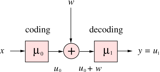
Figure 1: Coding-decoding diagram over a Gaussian channel.

In this paper, we consider the problem of distributed decision making with information constraints under linear quadratic settings. For instance, information constraints appear naturally when making decisions over networks. These problems can be formulated as team problems. Early results considered static team theory in stochastic settings [8], [9], [5]. In [2], the team problem with two team members was solved. The solution cannot be easily extended to more than two players since it uses the fact that the two members have common information; a property that doesn’t necessarily hold for more than two players. [2] uses the result to consider the two-player problem with one-step delayed measurement sharing with the neighbors, which is a special case of the partially nested information structure, where there is no signaling incentive. Also, a nonlinear team problem with two team members was considered in [1], where one of the team members is assumed to have full information whereas the other member has only access to partial information about the state of the world. Related team problems with exponential cost criterion were considered in [6]. Optimizing team problems with respect to affine decisions in a minimax quadratic cost was shown to be equivalent to stochastic team problems with exponential cost, see [3]. The connection is not clear when the optimization is carried out over nonlinear decision functions. In [4], a general solution was given for an arbitrary number of team members, where linear decision were shown to be optimal and can be found by solving a linear matrix inequality. In the deterministic version of Witsenhausen’s counterexample, that is minimizing the quadratic cost with respect to the worst case scenario of the state $x$ (instead of the assumption that $x$ is Gaussian), the linear decisions where shown to be optimal in [10].

We will show that for static linear quadratic minimax team problems, where the players in the team affect each others information structure through their decisions, linear decisions are optimal in general, and can be found by solving a linear matrix inequality.

II Main Results

The deterministic problem considered is a quadratic game between a team of players and nature. Each player has limited information that could be different from the other players in the team. This game is formulated as a minimax problem, where the team is the minimizer and nature is the maximizer. We show that if there is a solution to the static minimax team problem, then linear decisions are optimal, and we show how to find a linear optimal solution by solving a linear matrix inequality.

III Deterministic Team Problems with Signaling Incentive

Consider the following team decision problem

$$\inf_{\mu}\sup_{v\in\mathbb{R}^{p},0\neq w\in\mathbb{R}^{q}} \frac{L(w,u)}{\|w\|^{2}+\|v\|^{2}}$$ (1)

subject to $$y_{i}=\sum_{j=1}^{N}D_{ij}u_{j}+E_{i}w+v_{i}$$

$$u_{i}=\mu_{i}(y_{i})$$

$$\text{for }i=1,...,N,$$

where $u_{i}\in\mathbb{R}^{m_{i}}$ and $E_{i}\in\mathbb{R}^{p_{i}\times q}$, for $i=1,...,N$,

$L(w,u)$ is a quadratic cost given by

$$L(w,u)=\left[\begin{matrix}w\\ u\end{matrix}\right]^{T}\left[\begin{matrix}Q_{ww}&Q_{wu}\\ Q_{uw}&Q_{uu}\end{matrix}\right]\left[\begin{matrix}w\\ u\end{matrix}\right],$$

$Q_{uu}\in\mathbb{S}^{m}_{++}$, $m=m_{1}+\cdots+m_{N}$, and

$$\left[\begin{matrix}Q_{ww}&Q_{wu}\\ Q_{uw}&Q_{uu}\end{matrix}\right]\in\mathbb{S}^{m+n}_{+}.$$

The players $u_{1}$,…, $u_{N}$ make up a team, which plays against nature represented by the vector $w$, using $\mu\in\mathcal{C}$. This problem is more complicated than the static team decision problem studied in [4], since it has the same flavour as that of the Witsenhausen counterexample that was presented in the introduction. We see that the measurement $y_{i}$ of decision maker $i$ could be affected by the other decision makers through the terms $D_{ij}u_{j}$, $j=1,...,N$.

Note that we have the equality $y=Du+Ew+v$ which is equivalent to $v=Du+Ew-y$. Using this substitution of variable, the team problem (1) is equivalent to

$$\inf_{\mu\in\mathcal{C}}\sup_{y\in\mathbb{R}^{p},0\neq w\in\mathbb{R}^{q}} \frac{L(w,\mu(y))}{||D\mu(y)+Ew-y||^{2}+\|w\|^{2}}$$ (2)

Assumption 1

$$\gamma^{\star}\leq\bar{\gamma}:=\inf_{Du\neq 0}\hskip 2.84526pt\frac{u^{T}Q_{uu}u}{u^{T}D^{T}Du}.$$

Theorem 1

Let $\gamma^{\star}$ be the value of the game (1) and suppose that Assumption 1 holds. Then the following statements hold:

• There exist linear decisions $\mu_{i}(y_{i})=K_{i}y_{i}$, $i=1,...,N$, where the value $\gamma^{\star}$ is achieved.

• If $\gamma^{\star}<\bar{\gamma}$, then for any $\gamma\in[\gamma^{\star}~{},~{}\bar{\gamma})$, a linear decision $Ky$ with $K\in\mathbb{K}$ that achieves $\gamma$ is obtained by solving the linear matrix inequality

  find $$K$$

  subject to $$K=\text{diag}(K_{1},...,K_{N})$$

  $$C=\left[\begin{matrix}I&0\end{matrix}\right]\in\mathbb{R}^{p\times(p+q)},\hskip 8.53581ptQ_{uu}(\gamma)\in\mathbb{S}^{m\times m}$$

  $$\left[\begin{matrix}Q_{xx}(\gamma)&Q_{xu}(\gamma)\\ Q_{ux}(\gamma)&Q_{uu}(\gamma)\end{matrix}\right] =\left[\begin{matrix}Q_{ww}&0&Q_{wu}\\ 0&0&0\\ Q_{uw}&0&Q_{uu}\end{matrix}\right]-\gamma\left[\begin{matrix}E^{T}E&-E^{T}&-E^{T}D\\ -E&I&-D\\ -D^{T}E&-D^{T}&D^{T}D\par\end{matrix}\right]$$

  $$\left[\begin{matrix}Q_{xx}(\gamma)+Q_{xu}(\gamma)KC+C^{T}K^{T}Q_{ux}(\gamma)&C^{T}K^{T}\\ KC&-Q_{uu}^{-1}(\gamma)\end{matrix}\right]\preceq 0,$$

Proof:

($i$) Note that

$$y=Du+Ew+v\Longleftrightarrow v=y-Du-Ew\Rightarrow$$

$$\Rightarrow\frac{L(w,u)}{||v||^{2}+\|w\|^{2}}=\frac{L(w,u)}{||y-Du-Ew||^{2}+\|w\|^{2}}.$$

Now introduce $x\in\mathbb{R}^{n}$, $n=p+q$, such that

$$x=\left[\begin{matrix}w\\ y\end{matrix}\right],$$

and

$$Q =\left[\begin{matrix}Q_{ww}&0&Q_{wu}\\ 0&0&0\\ Q_{uw}&0&Q_{uu}\end{matrix}\right],$$ (3)

$$R =\left[\begin{matrix}E^{T}E&-E^{T}&-E^{T}D\\ -E&I&-D\\ -D^{T}E&-D^{T}&D^{T}D\par\end{matrix}\right].$$

Then,

$$J(x,u) :=\left[\begin{matrix}x\\ u\end{matrix}\right]^{T}Q\left[\begin{matrix}x\\ u\end{matrix}\right]=L(w,u),$$

$$F(x,u) :=\left[\begin{matrix}x\\ u\end{matrix}\right]^{T}R\left[\begin{matrix}x\\ u\end{matrix}\right]=||y-Du-Ew||^{2}+\|w\|^{2},$$

and $y=Cx.$ Hence, we have that

$$\frac{L(w,u)}{||v||^{2}+\|w\|^{2}}=\frac{L(w,u)}{||y-Du-Ew||^{2}+\|w\|^{2}}=\frac{J(x,u)}{F(x,u)}.$$

Then, for any $\gamma\in(\gamma^{\star}~{},~{}\bar{\gamma})$, there exists a decision function $\mu\in\mathcal{C}$ such that

$$J(x,\mu(Cx))-\gamma F(x,\mu(Cx))=\left[\begin{matrix}x\\ \mu(Cx)\end{matrix}\right]^{T}\left[\begin{matrix}Q_{xx}(\gamma)&Q_{xu}(\gamma)\\ Q_{ux}(\gamma)&Q_{uu}(\gamma)\end{matrix}\right]\left[\begin{matrix}x\\ \mu(Cx)\end{matrix}\right]\leq 0$$

for all $x$. Under Assumption 1, we have that

$$Q_{uu}(\gamma)=Q_{uu}-\gamma D^{T}D\succ 0$$

for any $\gamma\in(\gamma^{\star}~{},~{}\bar{\gamma}]$. Thus, we can apply Theorem 1 in [4], which implies that there must exist linear decisions that can achieve any $\gamma\in(\gamma^{\star}~{},~{}\bar{\gamma}]$. By compactness, there must exist linear decisions that achieve $\gamma^{\star}$.

($ii$) Let $\mu(Cx)=KCx$ for $K\in\mathbb{K}$. Then

$$\left[\begin{matrix}x\\ KCx\end{matrix}\right]^{T}\left[\begin{matrix}Q_{xx}(\gamma)&Q_{xu}(\gamma)\\ Q_{ux}(\gamma)&Q_{uu}(\gamma)\end{matrix}\right]\left[\begin{matrix}x\\ KCx\end{matrix}\right]\leq 0,~{}~{}\forall x$$

$$\Updownarrow$$

$$\left[\begin{matrix}I\\ KC\end{matrix}\right]^{T}\left[\begin{matrix}Q_{xx}(\gamma)&Q_{xu}(\gamma)\\ Q_{ux}(\gamma)&Q_{uu}(\gamma)\end{matrix}\right]\left[\begin{matrix}I\\ KC\end{matrix}\right]\preceq 0$$

$$\Updownarrow$$

$$Q_{xx}(\gamma)+Q_{xu}(\gamma)KC+C^{T}K^{T}Q_{ux}(\gamma)+C^{T}K^{T}Q_{uu}(\gamma)KC\preceq 0$$

$$\Updownarrow$$

$$\left[\begin{matrix}Q_{xx}(\gamma)+Q_{xu}(\gamma)KC+C^{T}K^{T}Q_{ux}(\gamma)&C^{T}K^{T}\\ KC&-Q_{uu}^{-1}(\gamma)\end{matrix}\right]\preceq 0,$$

and the proof is complete. ∎

IV Linear Quadratic Control with Arbitrary Information Constraints

Consider the dynamic team decision problem

$$\inf_{\mu}\sup_{w,v\neq 0} \frac{\sum_{k=1}^{M}\left[\begin{matrix}x(k)\\ u(k)\end{matrix}\right]^{T}\left[\begin{matrix}Q_{xx}&Q_{xu}\\ Q_{ux}&Q_{uu}\end{matrix}\right]\left[\begin{matrix}x(k)\\ u(k)\end{matrix}\right]}{\sum_{k=1}^{M}\|w(k)\|^{2}+\|v(k)\|^{2}}$$ (4)

subject to $$x(k+1)=Ax(k)+Bu(k)+w(k)$$

$$y_{i}(k)=C_{i}x(k)+v_{i}(k)$$

$$u_{i}(k)=[\mu_{k}]_{i}(y_{i}(k)),i=1,...,N.$$

Now write $x(t)$ and $y(t)$ as

$$x(t) =\sum_{k=1}^{t}A^{k}Bu(M-k)+\sum_{k=1}^{t}A^{k}w(M-k),$$

$$y_{i}(t) =\sum_{k=1}^{t}C_{i}A^{k}Bu(M-k)+\sum_{k=1}^{t}C_{i}A^{k}w(M-k)+v_{i}(k).$$

It is easy to see that the optimal control problem above is equivalent to a static team problem of the form (1). Thus, linear controllers are optimal under Assumption 1.

Example 1

Consider the deterministic version of the Witsenhausen counterexample presented in the introduction:

$$\inf_{\mu_{1},\mu_{2}} \gamma$$

s. t. $$\frac{{k^{2}}\mu_{1}^{2}(y_{1})+({x_{1}}-\mu_{2}(y_{2}))^{2}}{x_{0}^{2}+w^{2}}\leq\gamma$$

$${y_{1}=x_{0}}$$

$${x_{1}}={x_{0}}+\mu_{1}(y_{1})$$

$$y_{2}=x_{1}+w={x_{0}}+\mu_{1}(y_{1})+w$$

Substitue $x_{0}=y_{1}$, $x_{1}=y_{1}+\mu_{1}(y_{1})$ and $w^{2}=({x_{0}}+\mu_{1}(y_{1})-y_{2})^{2}$ in the inequality

$$\ {k^{2}}\mu_{1}^{2}(y_{1})+({x_{1}}-\mu_{2}(y_{2}))^{2}\leq\gamma({x_{0}^{2}}+w^{2}).$$

Then, we get the equivalent problem

$$\inf_{\mu_{1},\mu_{2}} \gamma$$

s. t. $${k^{2}}\mu_{1}^{2}(y_{1})+(y_{1}+\mu_{1}(y_{1})-\mu_{2}(y_{2}))^{2}\leq\gamma(y_{1}^{2}+(y_{1}+\mu_{1}(y_{1})-y_{2})^{2})$$

Completing the squares gives the following equivalent inequality

$$\left[\begin{matrix}y_{1}\\ y_{2}\\ \mu_{1}(y_{1})\\ \mu_{2}(y_{2})\end{matrix}\right]^{T}\left[\begin{matrix}1-2\gamma&\gamma&1-\gamma&-1\\ \gamma&-\gamma&\gamma&0\\ 1-\gamma&\gamma&{1+k^{2}-\gamma}&{-1}\\ -1&0&{-1}&{1}\end{matrix}\right]\left[\begin{matrix}y_{1}\\ y_{2}\\ \mu_{1}(y_{1})\\ \mu_{2}(y_{2})\end{matrix}\right]\leq 0$$

For $k^{2}=0.1$, we can search over $\gamma<\bar{\gamma}=k^{2}=0.1$, and we can use Theorem 1 to deduce that linear decisions are optimal, and can be computed by iteratively solving a linear matrix inequality, where the iterations are done with respect to $\gamma$. We find that

$${\gamma^{\star}\approx 0.0901},$$

$${\mu_{1}(y_{1})=-0.9001y_{1}},$$

$${\mu_{2}(y_{2})=-0.0896y_{2}}.$$

For $k^{2}=1$, we iterate with respect to $\gamma<1$, and we find optimal linear decisions given by

$${\mu_{1}(y_{1})} {=}{-0.3856y_{1}}$$

$${\mu_{2}(y_{2})} {=}{0.3840y_{2}}$$

$$\Downarrow$$

$$\gamma^{\star}=0.3820$$

Example 2

Consider the deterministic counterpart of the multi-stage finite-horizon stochastic control problem that was considered in [7]:

$$\inf_{\mu_{k}:\mathbb{R}\rightarrow\mathbb{R}}\sup_{x_{0},v_{0},...,v_{m-1}\in\mathbb{R}}\frac{(x_{m}-x_{0})^{2}+\sum_{k=0}^{m-2}\mu^{2}_{k}(y_{k})}{x_{0}^{2}+v_{0}^{2}+\cdots+v_{m-1}^{2}}$$

subject to the dynamics

$$x_{k+1} =\mu_{k}(y_{k})$$

$$y_{k} =x_{k}+v_{k}.$$

It is easy to check that $\bar{\gamma}=1$ and $Q_{uu}-\gamma D^{T}D\succ 0$ for $\gamma<\bar{\gamma}$ (compare with Assumption 1) . Thus, linear decisions are optimal. This is compared to the stochastic version, where linear decisions where not optimal for $m>2$.

V Conclusions

We have considered the static team problem in deterministic linear quadratic settings where the team members may affect each others information. We have shown that decisions that are linear in the observations are optimal and can be found by solving a linear matrix inequality.

For future work, it would be interesting to consider the case where the measurements are given by $y=Du+Ew+Fv$, for an arbitrary matrix $F$.

VI Acknowledgements

The author is grateful to Professor Anders Rantzer, Professor Bo Bernhardsson, and the reviewers for valuable comments and suggestions.

This work is supported by the Swedish Research Council.

References

• [1] P.Β Bernhard and N.Β Hovakimyan. Nonlinear robust control and minimax team problems. International Journal of Robust and Nonlinear Control, 9(9):239–257, 1999.
• [2] G.Β Didinsky and T.Β Basar. Minimax decentralized controllers for discrete-time linear systems. In 41st Conference on Decision and Control, pages 481–486, 1992.
• [3] C.Β Fan, J.Β L. Speyer, and C.Β R. Jaensch. Centralized and decentralized solutions of the linear-exponential-gaussian problem. IEEE Trans. on Automatic Control, 39(10):1986–2003, 1994.
• [4] A.Β Gattami, B.Β Bernhardsson, and A.Β Rantzer. Robust team decision theory. IEEE Tran. Automatic Control, 57(3):794 – 798, march 2012.
• [5] Y.-C. Ho and K.-C. Chu. Team decision theory and information structures in optimal control problems-part i. IEEE Trans. on Automatic Control, 17(1), 1972.
• [6] J.Β Krainak, J.Β L. Speyer, and S.Β I. Marcus. Static team problems-part i. IEEE Trans. on Automatic Control, 27(4):839–848, 1982.
• [7] G.Β M. Lipsa and N.Β C. Martins. Finite horizon optimal memoryless control of a delay in gaussian noise: A simple counterexample. In IEEE Conference on Decision and Control, pages 1628–1635, December 2008.
• [8] J.Β Marschak. Elements for a theory of teams. Management Sci., 1:127–137, 1955.
• [9] R.Β Radner. Team decision problems. Ann. Math. Statist., 33(3):857–881, 1962.
• [10] M.Β Rotkowitz. Linear controllers are uniformly optimal for the Witsenhausen counterexample. In IEEE Conference on Decision and Control, pages 553–558, 2006.
• [11] H.Β S. Witsenhausen. A counterexample in stochastic optimum control. SIAM Journal on Control, 6(1):138–147, 1968.