Analog readout for optical reservoir computers

Abstract

Reservoir computing is a new, powerful and flexible machine learning technique that is easily implemented in hardware. Recently, by using a time-multiplexed architecture, hardware reservoir computers have reached performance comparable to digital implementations. Operating speeds allowing for real time information operation have been reached using optoelectronic systems. At present the main performance bottleneck is the readout layer which uses slow, digital postprocessing. We have designed an analog readout suitable for time-multiplexed optoelectronic reservoir computers, capable of working in real time. The readout has been built and tested experimentally on a standard benchmark task. Its performance is better than non-reservoir methods, with ample room for further improvement. The present work thereby overcomes one of the major limitations for the future development of hardware reservoir computers.

${}^{\text{1}}$Service OPERA-photonique, Université Libre de Bruxelles (U.L.B.), 50 Avenue F. D. Roosevelt, CP 194/5, B-1050 Bruxelles, Belgium

${}^{\text{2}}$Department of Electronics and Information Systems (ELIS), Ghent University, Sint-Pietersnieuwstraat 41, 9000 Ghent, Belgium.

${}^{\text{3}}$Laboratoire d’Information Quantique (LIQ), Université Libre de Bruxelles (U.L.B.), 50 Avenue F. D. Roosevelt, CP 225, B-1050 Bruxelles, Belgium

1 Introduction

The term “reservoir computing” encompasses a range of similar machine learning techniques, independently introduced by H. Jaeger [1] and by W. Maass [2]. While these techniques differ in implementation details, they share the same core idea: that one can leverage the dynamics of a recurrent nonlinear network to perform computation on a time dependent signal without having to train the network itself. This is done simply by adding an external, generally linear readout layer and training it instead. The result is a powerful system that can outperform other techniques on a range of tasks (see for example the ones reported in [3, 4]), and is significantly easier to train than recurrent neural networks. Furthermore it can be quite easily implemented in hardware [5, 6, 7], although it is only recently that hardware implementations with performance comparable to digital implementations have been reported [8, 9, 10].

One great advantage of this technique is that it places almost no requirements on the structure of the recurrent nonlinear network. The topology of the network, as well as the characteristics of the nonlinear nodes, are left to the user. The only requirements are that the network should be of sufficiently high dimensionality, and that it should have suitable rich dynamics. The last requirement essentially means that the dynamics allows the exploration of a large number of network states when new inputs come in, while at the same time retaining for a finite time information on the previous inputs [11]. For this reason, the reservoir computers appearing in literature use widely different nonlinear units, see for example [1, 2, 5, 12] and in particular the time multiplexing architecture proposed in [7, 8, 9, 10].

Optical reservoir computers are particularly promising, as they can provide an alternative path to optical computing. They could leverage the inherent high speeds and parallelism granted by optics, without the need for strong nonlinear interaction needed to mimic traditional electronic components. Very recently, optoelectronic reservoir computers have been demonstrated by different research teams [10, 9], conjugating good computational performances with the promise of very high operating speeds. However, one major drawback in these experiments, as well as all preceding ones, was the absence of readout mechanisms: reservoir states were collected on a computer and post-processed digitally, severely limiting the processing speeds obtained and hence the applicability.

An analog readout for experimental reservoirs would remove this major bottleneck, as pointed out in [13]. The modular characteristics of reservoir computing imply that hardware reservoirs and readouts can be optimized independently and in parallel. Moreover, an analog readout opens the possibility of feeding back the output of the reservoir into the reservoir itself, which in turn allows the use of different training techniques [14] and to apply reservoir computing to new categories of tasks, such as pattern generation [15, 16].

In this paper we present a proposal for the readout mechanism for opto-electronic reservoirs, using an optoelectronic intensity modulator. The design that we propose will drastically cut down their operation time, specially in the case of long input sequences. Our proposal is suited to optoelectronic or all-optical reservoirs, but the concept can be easily extended to any experimental time-multiplexed reservoir computer. The mechanism has been tested experimentally using the experimental reservoir reported in [10], and compared to a digital readout. Although the results are preliminary, they are promising: while not as good as those reported in [10], they are however already better than non-reservoir methods for the same task [16].

2 Reservoir computing and time multiplexing

2.1 Principles of Reservoir Computing

The main component of a reservoir computer (RC) is a recurrent network of nonlinear elements, usually called “nodes” or “neurons”. The system typically works in discrete time, and the state of each node at each time step is a function of the input value at that time step and of the states of neighboring nodes at the previous time step. The network output is generated by a readout layer - a set of linear nodes that provide a linear combination of the instantaneous node states with fixed coefficients.

The equation that describes the evolution of the reservoir computer is

$$x_{i}(n)=f(\alpha m_{i}u(n)+\beta\sum_{j=1}^{N}w_{ij}x_{j}(n-1))$$ (1)

where $x_{i}(n)$ is the state of the $i$-th node at discrete time $n$, $N$ is the total number of nodes, $u(n)$ is the reservoir input at time $n$, $m_{i}$ and $w_{ij}$ are the connection coefficients that describe the network topology, $\alpha$ and $\beta$ are two parameters that regulate the network’s dynamics, and $f$ is a nonlinear function. One generally tunes $\alpha$ and $\beta$ to have favorable dynamics when the input to be treated is injected in the reservoir. The network output $y(n)$ is then constructed using a set of readout weights $W_{i}$ and a bias weight $W_{b}$, as

$$y(n)=\sum_{i=1}^{N}W_{i}x_{i}(n)+W_{b}$$ (2)

Training a reservoir computer only involves the readout layer, and consists in finding the best set of readout weights $W_{i}$ and bias $W_{b}$ that minimize the error between the desired output and the actual network output. Unlike conventional recurrent neural networks, the strength of connections $m_{i}$ and $w_{ij}$ are left untouched. As the output layer is made only of linear units, given the full set of reservoir states $x_{i}(n)$ for all the time steps $n$, the training procedure is a basic, regularized linear regression.

2.2 Time multiplexing

The number of nodes in a reservoir computer determines an upper limit to the reservoir performance [17]; this can be an obstacle when designing physical implementations of RCs, which should contain a high number of interconnected nonlinear units. A solution to this problem proposed in [7, 8], is time multiplexing: the $x_{i}(n)$ are computed one by one by a single nonlinear element, which receives a combination of the input $u(n)$ and a previous state $x_{j}(n-1)$. In addition an input mask $m_{i}$ is applied to the input $u(n)$, to enrich the reservoir dynamics. The value of $x_{i}(n)$ is then stored in a delay line to be used at a later time step $n+1$. The interaction between different neurons can be provided by either having a slow nonlinear element which couples state $x_{i}$ to the previous states $x_{i-1},x_{i-2},...$ [8], or by using an instantaneous nonlinear element and desynchronizing the input with respect to the delay line [10].

2.3 Hardware RC with digital readout

The hardware reservoir computer we use in the present work is identical to the one reported in [10] (see also [9]). It uses the time-multiplexing with desynchronisation technique described in the previous paragraph. We give a brief description of the experimental system, represented in the left part of Figure 1. It uses a $LiNbO_{3}$ Mach-Zehnder (MZ) modulator, operating on a constant power 1560 nm laser, as the nonlinear component. A MZ modulator is a voltage controlled optoelectronic device; the amount of light that it transmits is a sine function of the voltage applied to it. The resulting state $x_{i}(n)$ is encoded in a light intensity level at the MZ output. It is then stored in a spool of optical fiber, acting as delay line of duration $T=8.5\mu s$, while all the subsequent states $x_{i}(n)$ are being computed by the MZ modulator. When a state $x_{i}(n)$ reaches the end of the fiber spool it is converted into a voltage by a photodiode.

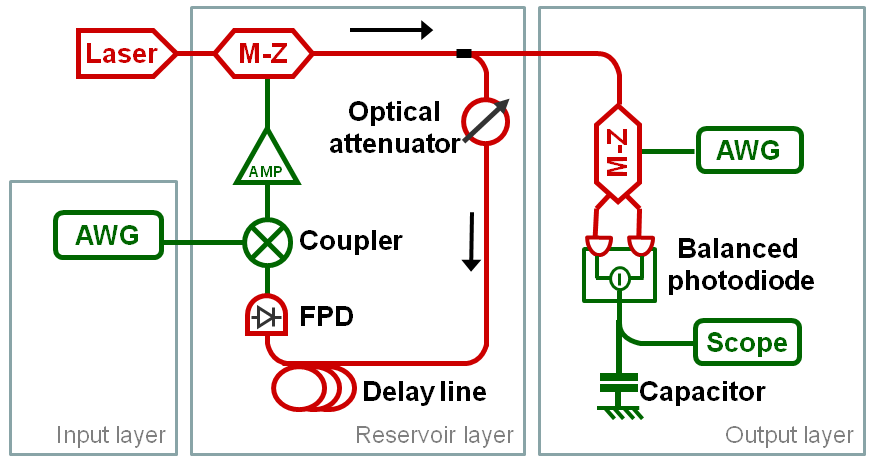
Figure 1: Scheme of the experimental setup, including the optoelectronic reservoir (’Input’ and ’Reservoir’ layers) and the analog readout (’Output’ layer). The red and green parts represent respectively the optical and electronic components. “AWG”: Arbitrary waveform generator. “M-Z”: $LiNbO_{3}$ Mach-Zehnder modulator. “FPD”: Feedback photodiode. “AMP”: Amplifier. “Scope”: NI PXI acquisition card.

The input $u(n)\mbox{ }$is multiplied by the input mask $m_{i}$ and encoded in a voltage level by an Arbitrary Waveform Generator (AWG). The two voltages corresponding to the state $x_{i}(n)$ at the end of the fiber spool and the input $m_{i}u(n)$ are added, amplified, and the resulting voltage is used to drive the MZ modulator, thereby producing the state $x_{j}(n+1)$, and so on for all values of $n$.

In the experiment reported in [10] a portion of the light coming out of the MZ is deviated to a second photodiode (not shown in Figure 1), that converts it into a voltage and sends it to a digital oscilloscope. The Mach-Zehnder output can be represented as “steps” of light intensities of duration $\theta$ (see Figure 2a), each one representing the value of a single node state $x_{i}$ at discrete time $n$. The value of each $x_{i}(n)$ is recovered by taking an average of the measured voltage for each state at each time step. The optimal readout weights $W_{i}$ and bias $W_{b}$ are then calculated on a computer from a subset (training set) of the recorded states, using ridge regression [18], and the output $y(n)$ is then calculated using equation 2 for all the states collected. The performance of the reservoir is then calculated by comparing the reservoir output $y(n)$ with the desired output $\hat{y}(n)$.

3 Analog readout

Readout scheme

Developing an analog readout for the reservoir computer described in section 2 means designing a device that multiplies the reservoir states shown in Figure 2a by the readout weights $W_{i}$, and that sums them together in such a way that the reservoir output $y(n)$ can be retrieved directly from its output. However, this is not straightforward to do, since obtaining good performance requires positive and negative readout weights $W_{i}.$ In optical implementations [10, 9] the states $x_{i}$ are encoded as light intensities which are always positive, so they cannot be subtracted one from another. Moreover, the summation over the states must include only the values of $x_{i}$ pertaining to the same discrete time step $n$ and reject all other values. This is difficult in time-multiplexed reservoirs, where the states $x_{N}(n)$ and $x_{1}(n+1)$ follow seamlessly.

Here we show how to resolve both difficulties using the scheme depicted in the right panel of Figure 1. Reservoir states encoded as light intensities in the optical reservoir computer and represented in Figure 2a are fed to the input of a second MZ modulator with two outputs. A second function generator governs the bias of the second Mach-Zehnder, providing the modulation voltage $V(t)$. The modulation voltage controls how much of the input light passing through the readout Mach-Zehnder is sent to each output, keeping constant the sum of the two output intensities. The two outputs are connected to the two inputs of a balanced photodiode, which in turn gives as output a voltage level proportional to the difference of the light intensities received at its two inputs. This allows us to multiply the reservoir states by both positive and negative weights.

The time average of the output voltage of the photodiode is obtained by using a capacitor. The characteristic time of the analog integrator $\tau$ is proportional to the capacity $C$. The role of this time scale is to include in the readout output all the pertinent contributions and exclude the others. The final output of the reservoir is the voltage across the capacitor at the end of each discretized time $n$.

What follows is a detailed description of the readout design.

Multiplication by arbitrary weights

The multiplication of the reservoir states by arbitrary weights, positive or negative, is realized by the second MZ modulator followed by the balanced photodiode. The modulation voltage $V(t)$ that drives the second Mach Zehnder is piecewise constant, with a step duration equal to the duration $\theta$ of the reservoir states; transitions in voltages and in reservoir states are synchronized. The modulation voltage is also a periodic function of period $\theta N$, so that each reservoir state $x_{i}(n)$ is paired with a voltage level $V_{i}$ that doesn’t depend on $n$. The light intensities $O_{1}(t)$ and $O_{2}(t)$ at the two outputs of the Mach-Zehnder modulator are

$$O_{1}(t)=I(t)\frac{1+\cos((V(t)+V_{bias})\frac{\pi}{V_{\pi}}+\varphi)}{2},O_{2}(t)=I(t)\frac{1-\cos((V(t)+V_{bias})\frac{\pi}{V_{\pi}}+\varphi)}{2},$$ (3)

where $I(t)$ is the light intensity coming from the reservoir, $V_{bias}$ is a constant voltage that drives the modulator, $\varphi$ is an arbitrary, constant phase value, and $V_{\pi}$ is the half-wave voltage of the modulator. Neglecting the effect of any bandpass filter in the photodiode, and choosing $V_{bias}$ appropriately, the output $P(t)$ from the photodiode can be written as

$$P(t)=G(O_{1}(t)-O_{2}(t))=I(t)(G\sin(\frac{V(t)\pi}{V_{\pi}}))=I(t)W(t)$$ (4)

with $G\mbox{ }$a constant gain factor. In other words, by setting the right bias and driving the modulator with a voltage $V(t)$, we multiply the signal $I(t)$ by an arbitrary coefficient $W(t)$. Note that, if $V(t)$ is piecewise constant, then $W(t)$ is as well. This allows us to achieve the multiplication of the states $x_{i}(n)$, encoded in the light intensity $I(t)$, by the weights $W_{i}$, just by choosing the right voltage $V(t)$, as shown in Figure 2b.

Summation of weighted states

To achieve the summation over all the states pertaining to the same discrete time step $n,$ which according to equation 2 will give us the reservoir output minus the bias $W_{b}$, we use the capacitor at the right side of the Output layer in Figure 1. The capacitor provides the integration of the photodiode output given by eq. 4 with an exponential kernel and time constant $\tau$. If $\tau$ is significantly less than the amount of time $\theta N$ needed for the system to process all the nodes relative to a single time step, we can minimize the crosstalk between node states relative to different time steps.

Let us consider the input $I(t)$ of the readout, and let $t=0$ be the instant where the state of the first node for a given discrete time step $n$ begins to be encoded in $I(t)$ . Using equation 4, we can write the voltage $Q(t)$ on the capacitor at time $\theta N$ as

$$Q(\theta N)=Q(0)e^{-\frac{\theta N}{\tau}}+\int_{0}^{\theta N}I(s)W(s)e^{-\frac{\theta N-s}{\tau}}ds$$ (5)

For $0<t<\theta N$, we have

$$I(t)=x_{i}(n),W(t)=w_{i},\>\mbox{for}\>\theta(i-1)<t<\theta i$$ (6)

Integrating equation 5 yields

$$Q(\theta N)=Q(0)e^{-\frac{\theta N}{\tau}}+\sum_{i=1}^{N}x_{i}(n)\eta_{i}w_{i},\>\>\eta_{i}=e^{-\frac{\theta(N-i)}{\tau}}(1-e^{-\frac{\theta}{\tau}})\tau$$ (7)

Equation 7 shows that, at time $\theta N$, the voltage on the capacitor is a linear combination of the reservoir states for the discrete time $n$, with node-dependent coefficients $\eta_{i}w_{i}$, plus a residual of the voltage at time $0$, multiplied by an extinction coefficient $e^{-\frac{\theta N}{\tau}}$. At time $2\theta N$ the voltage on the capacitor would be a linear combination of the states for discrete time $n+1$, multiplied by the same coefficients, plus a residual of the voltage at time $\theta N$, and so on for all values of $n$ and corresponding multiples of $\theta N$.

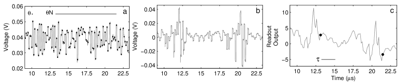
Figure 2: a) Reservoir output $I(t)$. The gray line represents the output as measured by a photodiode and an oscilloscope. We indicated for reference the time $\theta=130ns$ used to process a single node and the duration $\theta N=8.36\mu s$ of the whole set of states. b) Output $P(t)$ of the balanced photodiode (see equation 4), with the trace of panel a) as input, before integration. c) Voltage $Q(t)$ on the capacitor for the same input (see equation 5). The integration time $\tau$ is indicated for reference. The black dots indicate the values at the end of each discretized time $n$, taken as the output $y(n)$of the analog readout.

A simple procedure would encode the weights $w_{i}=\frac{W_{i}}{\eta_{i}}$ onto the voltage $V(t)$ that drives the modulator , provide an external, constant bias $W_{b}$, and have the output $y(n)$ of the reservoir, defined by equation 2, effectively encoded on the capacitor. This simple procedure would however be unsatisfactory because unavoidably some of the $\eta_{i}$ would be very small, and therefore the $w_{i}$ would be large, spanning several orders of magnitude. This is undesirable, as it requires a very precise control of the modulation voltage $V(t)$ in order to recreate all the $w_{i}$ values, leaving the system vulnerable to noise and to any non-ideal behavior of the modulator itself.

To mitigate this, we adapt the training algorithm based on ridge regression to our case. We redefine the reservoir states as $\xi_{i}(n)=x_{i}(n)\eta_{i}$; we then calculate the weights $\omega_{i}$ that, applied to the states $\xi_{i}$, give the best approximation to the desired output $\hat{y}(n)$. The advantage here is that ridge regression keeps the norm of the weight vector to a minimum; by redefining the states, we can take the $\eta_{i}$ into account without having big values of $w_{i}$ that force us to be extremely precise in generating the readout weights.

A sample trace of the voltage on the capacitor is shown in Figure 2c.

Hardware implementation

To implement the analog readout, we started from the experimental architecture described in Section 2, and we added the components depicted in the right part of Figure 1. For the weight multiplication, we used a second Mach-Zehnder modulator (Photline model MXDO-LN-10 with bandwidth in excess of 10GHz and $V_{\pi}=5.9V$), driven by a Tabor 2074 Arbitrary Waveform Generator (maximum sampling rate 200 MSamples/s). The two outputs of the modulator were fed into a balanced photodiode (Terahertz technologies model 527 InGaAs balanced photodiode, bandwidth set to 125MHz, response set to 1000V/W), whose output was read by the National Instruments PXI digital acquisition card (sampling rate 200 MSamples/s).

In most of the experimental results described here, the capacitor at the end of the circuit was simulated and not physically inserted into the circuit: this allowed us to quickly cycle in our experiments through different values of $\tau$ without taking apart the circuit every time. The external bias $W_{b}$ to the output, introduced in equation 2, was also provided after the readout. The reasoning behind these choices is that both these implementations are straightforward, while the use of a modulator and a balanced photodiode as a weight generator is more complex: we chose to focus on the latter issue for now, as our goal is to validate the proposed architecture.

4 Results

As a benchmark for our analog readout, we use a wireless channel equalization task, introduced in 1994 [19] to test adaptive bilinear filtering and subsequently used by Jaeger [16] to show the capabilities of reservoir computing. This task is becoming a standard benchmark task in the reservoir computing community, and has been used for example in [20]. It consists in recovering a sequence of symbols transmitted along a wireless channel, in presence of multiple reflections, noise and nonlinear distortion; a more detailed description of the task can be found in the Appendix. The performance of the reservoir is usually measured in Symbol Error Rate (SER), i.e. the rate of misinterpreted symbols, as a function of the amount of noise in the wireless channel.

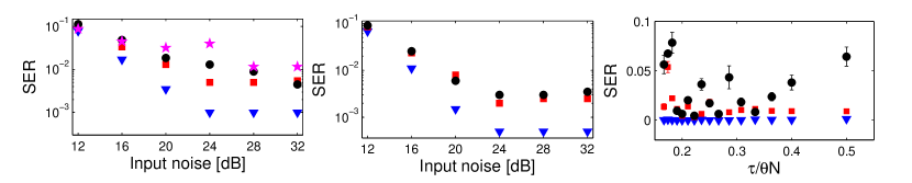
Figure 3: Performance of the analog readout. Left: Performance as a function of the input SNR, for a reservoir of 28 nodes, with $\tau/\theta N=0.18$. Middle: Performance for the same task, for a reservoir of 64 nodes, $\tau/\theta N=0.18$. Right: Performance as a function of the ratio $\tau/\theta N$, at constant input noise level (28 dB SNR) for a reservoir of 64 nodes. The performance is measured in Signal Error Rate (SER). Blue triangles: reservoir with digital readout. Red squares: reservoir with ideal analog readout. Black circles: reservoir with experimental analog readout (simulated capacitor). Purple stars in the left panel: reservoir where a physical capacitor has been used.

Figure 3 shows the performance of the experimental setup of [10] for a network of 28 nodes and one of 64 nodes, for different amounts of noise. For each noise level, three quantities are presented. The first is the performance of the reservoir with a digital readout (blue triangles), identical to the one used in [10]. The second is the performance of a simulated, ideal analog readout, which takes into account the effect of the $\eta_{i}$ coefficients introduced in equation 7, but no other imperfection. It produces as output the discrete sum $\omega_{b}+\sum_{i=1}^{N}\xi_{i}\omega_{i}$ (red squares). This is, roughly speaking, the goal performance for our experimental readout. The third and most important is the performance of the reservoir as calculated on real data taken from the analog reservoir with the analog output, with the effect of the continuous capacitive integration computed in simulation (black circles).

As can be seen from the figure, the performance of the analog readout is fairly close to its ideal value, although it is significantly worse than the performance of the digital readout. However, it is already better than the non-reservoir methods reported in [19] and used by Jaeger as benchmarks in [16]. It can also handle higher signal-to-noise ratios. As expected, networks with more nodes have better performance; it should be noted, however, that in experimental reservoirs the number of nodes cannot be raised over a certain threshold. The reason is that the total loop time $\theta N$ is determined by the experimental hardware (specifically, the length of the delay line); as $N$ increases, the length $\theta$ of each node must decrease. This leaves the experiment vulnerable to noise and bandpass effect, that may lead, for example, to an incorrect discretization of the $x_{i}(n)$ values, and an overall worse performance.

We did test our readout with a $70nF$ capacitor, with a network of 28 nodes, to prove that the physical implementation of our concept is feasible: the performance of this setup is shown in the left panel of Figure 3. The results are comparable to those obtained in simulation, even if, at low levels of noise in the input, the performance of the physical setup is slightly worse.

The rightmost panel of figure 3 shows the effects of the choice of the capacitor at the end of the circuit, and therefore of the value of $\tau$. The plot represents the performance at 28 dB SNR for a network of 64 nodes, for different values of the ratio $\tau/\theta N$, obtained by averaging the results of 10 tests. It is clear that the choice of $\tau$ has a complicated effect on the readout performance; however, some general rules may be inferred. Too small values of $\tau$ mean that the contribution from the very first nodes is vanishingly small, effectively decreasing the reservoir dimensionality, which has a strong impact on the performance both of the ideal and the experimental reservoir. On the other hand, larger values of $\tau$ impact the performance of the experimental readout, as the residual term in equation 7 gets larger. A compromise value of $\tau/\theta N=0.222$ seems to give the best result, corresponding in our case to a capacity of about $70$ nF.

5 Discussion

To our knowledge, the system presented here is the first analog readout for an experimental reservoir computer. While the results presented here are preliminary, and there is much optimization of experimental parameters to be done, the system already outperforms non-reservoir methods. We expect to extend easily this approach to different tasks, already studied in [9, 10], including a spoken digit recognition task on a standard dataset.

Further performance improvements can reasonably be expected from fine-tuning of the training parameters: for instance the amount of regularization in the ridge regression procedure, that here is left constant at $1\cdot 10^{-4}$, should be tuned for best performance. Adaptive training algorithms, such as the ones mentioned in [21], could also take into account nonidealities in the readout components. Moreover the choice of $\tau,$ as Figure 3 shows, is not obvious and a more extensive investigation could lead to better performance.

The architecture proposed here is simple and quite straightforward to realize. It is very modular, meaning that it can be added at the output of any preexisting time multiplexing reservoir with minimal effort, whether it is based on optics or electronics. The capacitor at the end of the circuit could probably be substituted with a more complicated, active electronic circuit performing the summation of the incoming signal before resetting itself. This would eliminate the problem of residual voltages, and allow better performance at the cost of increased complexity of the readout.

The main interest of the analog readout is that it allows optoelectronic reservoir computers to fully leverage their main characteristic, which is the speed of operation. Indeed, removing the need for slow, offline postprocessing is indicated in [13] as one of the major challenges in the field. Once the training is finished, optoelectronic reservoirs can process millions of nonlinear nodes per second [10]; however, in the case of a digital readout, the node states must be recovered and postprocessed to obtain the reservoir outputs. It takes around $1.6$ seconds for the digital readout in our setup to retrieve and digitize the states generated by a 9000 symbol input sequence. The analog readout removes the need for postprocessing, and can work at a rate of about $8.5$ $\mu s$ per input symbol, five orders of magnitude faster than the electronic reservoir reported in [8].

Finally, having an analog readout opens the possibility of feedback - using the output of the reservoir as input or part of an input for the successive time steps. This opens the way for different tasks to be performed [15] or different training techniques to be employed [14].

Appendix: Nonlinear Channel Equalization task

What follows is a detailed description of the channel equalization task used to test the reservoir performance. The goal for this task is to reconstruct a sequence $d(n)$ of symbols taken from $\{-3,-1,1,3\}$. The symbols in $d(n)$ are mixed together in a new sequence $q(n)$ given by

$$q(n) = 0.08d(n+2)-0.12d(n+1)+d(n)+0.18d(n-1)-0.1d(n\text{-}2)$$

$$+0.091d(n-3)\text{-}0.05d(n-4)+0.04d(n-5)+0.03d(n-6)+0.01d(n\text{-}7)$$

which models a wireless signal reaching a receiver through different paths with different traveling times. A noisy, distorted version $u(n)$ of the mixed signal $q(n)$, simulating the nonlinearities and the noise sources in the receiver, is created by having $u(n)=q(n)+0.036q(n)^{2}-0.011q(n)^{3}+\nu(n)$, where $\nu(n)$ is an i.i.d. Gaussian noise with zero mean adjusted in power to yield signal-to-noise ratios ranging from 12 to 32 dB. The sequence $u(n)$ is then fed to the reservoir as an input; the output of the readout $R(n)$ is rounded off to the closest value among $\{-3,-1,1,3\}$, and then compared to the desired symbol $d(n)$. The performance is usually measured in Signal Error Rate (SER), or the rate of misinterpreted symbols.

References

- [1] Jaeger, H. The "echo state" approach to analysing and training recurrent neural networks. Technical report, Technical Report GMD Report 148, German National Research Center for Information Technology, 2001.
- [2] Maass, W., Natschlager, T., and Markram, H. Real-time computing without stable states: A new framework for neural computation based on perturbations. Neural computation, 14(11):2531–2560, 2002.
- [3] Schrauwen, B., Verstraeten, D., and Van Campenhout, J. An overview of reservoir computing: theory, applications and implementations. In Proceedings of the 15th European Symposium on Artificial Neural Networks, pages 471–482, 2007.
- [4] Lukosevicius, M. and Jaeger, H. Reservoir computing approaches to recurrent neural network training. Computer Science Review, 3(3):127–149, 2009.
- [5] Fernando, C. and Sojakka, S. Pattern recognition in a bucket. Advances in Artificial Life, pages 588–597, 2003.
- [6] Schurmann, F., Meier, K., and Schemmel, J. Edge of chaos computation in mixed-mode vlsi - a hard liquid. In In Proc. of NIPS. MIT Press, 2005.
- [7] Paquot, Y., Dambre, J., Schrauwen, B., Haelterman, M., and Massar, S. Reservoir computing: a photonic neural network for information processing. volume 7728, page 77280B. SPIE, 2010.
- [8] Appeltant, L., Soriano, M. C., Van der Sande, G., Danckaert, G., Massar, S., Dambre, J., Schrauwen, B., Mirasso, C. R., and Fischer, I. Information processing using a single dynamical node as complex system. Nature Communications, 2:468, 2011.
- [9] Larger, L., Soriano, M. C., Brunner, D., Appeltant, L., Gutierrez, J. M., Pesquera, L., Mirasso, C. R. , and Fischer, I. Photonic information processing beyond Turing: an optoelectronic implementation of reservoir computing. Optics Express, 20(3):3241, 2012.
- [10] Paquot, Y., Duport, F., Smerieri, A., Dambre, J., Schrauwen, B., Haelterman, M., and Massar, S. Optoelectronic reservoir computing. Scientific reports, 2:287, January 2012.
- [11] Legenstein, R. and Maass, W. What makes a dynamical system computationally powerful? In Simon Haykin, José C. Principe, Terrence J. Sejnowski, and John McWhirter, editors, New Directions in Statistical Signal Processing: From Systems to Brain. MIT Press, 2005.
- [12] Vandoorne, K., Fiers, M., Verstraeten, D., Schrauwen, B., Dambre, J., and Bienstman, P. Photonic reservoir computing: A new approach to optical information processing. In 2010 12th International Conference on Transparent Optical Networks, pages 1–4. IEEE, 2010.
- [13] Woods, D. and Naughton, T. J. Optical computing: Photonic neural networks. Nature Physics, 8(4):257–259, April 2012.
- [14] Sussillo, D. and Abbott, L. F. Generating coherent patterns of activity from chaotic neural networks. Neuron, 63(4):544–57, 2009.
- [15] Jaeger, H., Lukosevicius, M., Popovici, D., and Siewert, U. Optimization and applications of echo state networks with leaky-integrator neurons. Neural networks : the official journal of the International Neural Network Society, 20(3):335–52, 2007.
- [16] Jaeger, H. and Haas, H. Harnessing nonlinearity: predicting chaotic systems and saving energy in wireless communication. Science, 304(5667):78–80, 2004.
- [17] Verstraeten, D., Dambre, J., Dutoit, X., and Schrauwen, B. Memory versus non-linearity in reservoirs. In The 2010 International Joint Conference on Neural Networks (IJCNN), pages 1–8. IEEE, 2010.
- [18] Wyffels, F. and Schrauwen, B. Stable output feedback in reservoir computing using ridge regression. Artificial Neural Networks-ICANN, pages 808–817, 2008.
- [19] Mathews. V. J. Adaptive algorithms for bilinear filtering. Proceedings of SPIE, 2296(1):317–327, 1994.
- [20] Rodan, A., and Tino, P. Minimum complexity echo state network. IEEE transactions on neural networks, 22(1):131–44, January 2011.
- [21] Legenstein, R., Chase, S. M., Schwartz, A. B., and Maass, W. A reward-modulated hebbian learning rule can explain experimentally observed network reorganization in a brain control task. The Journal of neuroscience : the official journal of the Society for Neuroscience, 30(25):8400–10, 2010.