Condensation of the scalar field with Stuckelberg and Weyl Corrections in the background of a planar AdS-Schwarzschild black hole

Abstract

We study analytical properties of the Stuckelberg holographic superconductors with Weyl corrections. We obtain the minimum critical temperature as a function of the mass of the scalar field $m^{2}$. We show that in limit of the $m^{2}=-3$,$T^{Min}_{c}\approx 0.158047\sqrt[3]{\rho}$ which is close to the numerical estimate $T_{c}^{Numerical}\approx 0.170\sqrt[3]{\rho}$. Further we show that the mass of the scalar field in bounded from below by the $m^{2}>m_{c}^{2}$ where $m_{c}^{2}=-5.40417$. This lower bound is weaker and different from the previous lower bound $m^{2}=-3$ predicted by stability analysis. We show that in the Breitenlohner-Freedman bound, the critical temperature remains finite. Explicitly, we prove that here there is exist a linear relation between $<O_{\Delta}>$ and the chemical potential.

I Introduction

The anti de Sitter/conformal field theory (AdS/CFT) correspondence conjecture maldacena is a very powerful tool for condensed matter physics specially for critical behavior of systems(see for instance condencesd1 ; condencesd2 and references therein) in high temperature superconductors super1 ; super2 . Different kinds of the holographic superconductors have been studied in Einstein theory GR1 ; GR2 or extended versions such as Gauss-Bonnet (GB)GB1 ; GB2 ; GB3 ; GB4 ; GB5 and even in Horava-Lifshitz theory HL1 ; HL2 . Further the effect of magnetic fields on superconductors have been discussed wen1 ; wen2 ; epl1 . There are some other types of superconductors with non linear Maxwell fields born1 ; born2 or with Chern-Simon terms cs . Also holographic superconductor models with the Maxwell field strength corrections have been investigated maxwell . Even, recently the holographic approach has been used for Josephson Junction effect cai2012 .
AdS/CFT can also describe superfluid states in which the condensing operator is a vector and hence rotational symmetry is broken, such states are termed p-wave superfluid states pwave1 ; pwave2 ; pwave3 . Here the CFT has a global $SU(2)$ symmetry and hence three conserved currents $J^{\mu}_{a}$ , where $a=1,2,3$ label the generators of $SU(2)$. Many of these works are based on a numerical analysis of the equations of motion (EOM) near the horizon and the asymptotic limit by a suitable shooting method. The pioneering work on analytic methods in this topic was by Hertzog herzog . He showed that at least in probe limit, by solving equations analytically (the perturbation theory), one can obtain the critical exponent and the expectation values of the dual operators. Near the critical point the value of the scalar field $\psi$ is small and consequently we can treat the expectation values of the dual boundary operators $\epsilon\equiv<O_{\Delta_{\pm}}>$ as a perturbation parameter. This method has been used recently by Kanno for investigating the GB superconductors even away from the probe limit kanno . Applying the analytical methods has lead to new trends (see for example analytic1 ; analytic2 and the references in it). There is a much more beatiful variational method to study the critical behavior of holographic superconductors analytic1 ; analytic2 . Instead of using shooting numerical algorithms, we can obtain the critical temperature $T_{c}$ and the exponent of the criticality by computing a simple variational approach. They studied different modes of super criticality s-wave, p-wave and even d-wave. Thus as we know, there are two major methods for analytical study of superconductors:

1- The small parameter perturbation theory herzog 2- The Sturm Liouville variational method analytic1 ; analytic2 . We must mention here that, the variational method, which has been used in the present work, gives only the minimum value of the critical temperature $T^{Min}_{c}$ for a model with a typical parameter. For example if we focus on Weyl corrections to holographic superconductors, as shown in weyl , for a large range of the coupling value $-\frac{1}{16}<\gamma<\frac{1}{24}$, there is a universal relation for the critical temperature $T_{c}\simeq\sqrt[3]{\rho}$. The proportionality constant depends on the Weyl coupling $\gamma$ and can be computed . In this case we found that temperature $T^{Min}_{c}=0.170\sqrt[3]{\rho}$ corresponds to the value $\gamma=-0.06$. In a recent paper, we showed that this critical temperature can be obtained from the variational method mpla .
Recently there is much interest on GB and Weyl corrected and specially the Stuckelberg superconductors, even in the presence of the external magnetic fields jian2010 . Recently, we investigated the p-wave holographic superconductors with Weyl corrections epl2 . The Stuckelberg holographic superconductors with Weyl corrections have been studied recently plb2011 . They studied the problem numerically. Our program in this paper is studying the Weyl corrections to the Stuckelberg superconductors analytically.

Our plan is organized as follows. In section 2, we construct the basic model of the $3+1$ holographic superconductor with Weyl corrections. In section 3 we present the analytical results for the condensation and minimum value of the critical temperature for different scaling and the critical exponent $\beta$ via variational bound. Conclusions and discussions follow in section 4.

II Weyl corrected Stuckelberg holographic superconductors

The s-wave Stuckelberg holographic superconductors constructed from an Abelian $U(1)$ gauge field coupled to a massive charged (complex) scalar field. The simplest form of the action in five dimensions ($3+1$ holographic picture) with Weyl corrections is plb2011

$$S=\int dtd^{4}x\sqrt{-g}(R+\frac{12}{l^{2}}-L).$$ (1)

with modified matter Lagrangian and Stuckelberg potental function $F(\psi)$,

$$L=\frac{1}{4}(F^{\mu\nu}F_{\mu\nu}-4\gamma C^{\mu\nu\rho\sigma}F_{\mu\nu}F_{\rho\sigma})+\frac{\partial_{\mu}\psi\partial^{\mu}\psi}{2}+\frac{m^{2}\psi^{2}}{2}+\frac{1}{2}F(\psi)A_{\mu}A^{\mu}.$$ (2)

The general form of the function $F(\psi)$ is

$$F(\psi)=\psi^{2}+c_{\alpha}\psi^{\alpha}+c_{4}\psi^{4}.$$ (3)

Here $3\leq\alpha\leq 4$ and $c_{4},c_{\alpha}$ are two constants of order $O(1)$. We write the action in units $2\kappa^{2}=1,$ in which the anti de-Sitter (AdS) radius $l=1$, the negative cosmological constant in this units is just $12$, charge $e=1$, $F_{\mu\nu}=\partial_{\mu}A_{\nu}-\partial_{\nu}A_{\mu}$. The gauge field $A_{\mu}$ lives in bulk and produces a conserved current $J^{\mu}$. This current corresponds to a global $U(1)$ symmetry. For this reason, $\psi$ is a real function. About the action (1) we can say that since the background geometry will be an Einstein metric, we will argue that there is a unique tensorial structure correcting the Maxwell term at leading order in derivatives, arising from a coupling to the Weyl tensor and leading to the dimension-six operator in (1) parametrized by the constant $\gamma$. Other curvature couplings simply provide constant shifts when considering linearized gauge field fluctuations about the background. There is another reason for considering the Weyl correction, which is related to the quantum corrections. In any background in which additional charged matter fields are integrated out below their mass threshold, the Weyl coupling $C^{\mu\nu\rho\sigma}F_{\mu\nu}F_{\rho\sigma}$ is generated at 1-loop, with a coefficient $\gamma=\frac{\alpha}{m^{2}}$ first computed (for four dimension) by Drummond and Hathrell qc . The Weyl’s coupling $\gamma$ is limited since its value lies in the interval $-\frac{1}{16}<\gamma<\frac{1}{24}$. In the probe limit, we neglect from the back reactions and in this case, the gravity sector is effectively decoupled from the matter field’s sector. In this probe limit, the exact solution for Einstein equations is a planer AdS-Schwarzschild black hole given by

$$ds^{2}=r^{2}(-fdt^{2}+dx^{i}dx_{i})+\frac{dr^{2}}{r^{2}f},$$ (4)

here

$$f=1-(\frac{h}{r})^{4},$$ (5)

and the horizon is located at $r=h$. This solution is asymptotically anti-de Sitter. The temperature of the dual conformal field theory is nothing but the Hawking temperature $T=\frac{h}{\pi}$. The numerical analysis of the phase transition for this model has been discussed recently plb2011 . When the temperature of the black hole falls below a critical value $T_{c}$, a phase transition occurs between the normal phase and a new phase, in which the scalar field $\psi$ condenses. If the model has this solution, we conclude that our field theory has a superfluid phase. We choose a gauge as $\psi=\psi(r),A_{t}=\varphi(r)$. It is more convenient to work in terms of the dimensionless parameter $\xi=\frac{h}{r}$, in which the horizon is $\xi=1$ and the boundary at infinity located at $\xi=0$. The resulting equations for metric (4) are given by plb2011

$$\psi^{\prime\prime}+\Big{(}\frac{f^{\prime}}{f}+\frac{5}{r}\Big{)}\psi^{\prime}+\frac{\phi^{2}}{2r^{4}f^{2}}\frac{dF}{d\psi}-\frac{m^{2}\psi}{r^{2}f}=0$$ (6)

$$\ \ \Big{(}1-\frac{24\gamma h^{4}}{r^{4}}\Big{)}\phi^{\prime\prime}+\Big{(}\frac{3}{r}+\frac{24\gamma h^{4}}{r^{5}}\Big{)}\phi^{\prime}-\frac{F}{r^{2}f}\phi=0$$ (7)

where prime denotes derivative with respect to $r$. In terms of the $\xi$, Eqs. (6), (7) become

$$\frac{d}{d\xi}\Big{(}\xi^{2}\frac{d\psi}{d\xi}\Big{)}-\frac{\xi(5-\xi^{4})}{1-\xi^{4}}\frac{d\psi}{d\xi}+\frac{\phi^{2}\xi^{2}}{2h^{2}(1-\xi^{4})^{2}}\frac{dF(\psi)}{d\psi}-\frac{m^{2}}{1-\xi^{4}}\psi=0,$$ (8)

$$\ \ (1-24\gamma\xi^{4})\frac{d}{d\xi}\Big{(}\xi^{2}\frac{d\phi}{d\xi}\Big{)}-3\xi(1+8\gamma\xi^{4})\frac{d\phi}{d\xi}-\frac{F(\psi)\phi}{1-\xi^{4}}=0$$ (9)

It is helpful to compare the analytical results with numerical results presented in plb2011 . For stability of the theory, we fix the mass of the scalar field above the Breitenlohner-Freedman (BF) bound BF . This BF bound is a lower bound on the mass of the scalar field $m^{2}$. For a theory defined in $d+1$ dimensions, the upper bound on the mass reads $m_{BF}^{2}=-\frac{d(d-1)}{4}$. This bound comes from the stability analysis. In this paper, from holographic picture of s-wave superconductors we will present another upper bound independent from this bound. Back to our model, the adequate and sufficient boundary conditions for these equations can be written on horizon $\xi=1$, the bulk’s boundary $\xi=0$. On the horizon we have $\varphi(1)=0,\psi^{\prime}(1)=\frac{2}{3}\psi(1)$ and on the boundary of bulk, the asymptotic forms of the solutions are

$$\varphi\approx\mu-\frac{\rho}{h}\xi^{2}$$ (10)

$$\psi\approx\epsilon\xi^{\Delta_{\pm}}=\psi^{(1)}\xi^{\Delta_{+}}+\psi^{(3)}\xi^{\Delta_{-}},$$ (11)

here

$$\epsilon=\frac{<O_{\Delta_{\pm}}>}{\sqrt{2}h^{\Delta_{\pm}}}$$

$\mu$ and $\rho$ are dual to the chemical potential and charge density of the boundary CFT, $\psi^{(1)}$ and $\psi^{(3)}$ are dual to the source and expectation value of the boundary operator $O$ respectively. $<O_{\Delta_{\pm}}>$ are the condensation with dimension $\Delta_{\pm}$ where

$$\Delta_{\pm}\equiv\Delta=\{3,1\}.$$ (12)

The conformal scaling dimension $\Delta\geq 1$ is related to the mass and the de Sitter radius by $m^{2}=\triangle(\triangle-4)$.

III Analytical results for the condensation and critical temperature

We know that there is a second order continuous phase transition at the critical temperature, the solution of Eq.(9) at $T_{c}$ is

$$\phi=\lambda h_{c}(1-\xi^{2})$$ (13)

where $h_{c}$ is the radius of the horizon at $T=T_{c}$. As $T\rightarrow T_{c}$, the scalar filed’s equation of motion (8) takes the following form

$$-\psi^{\prime\prime}+g(z)\psi^{\prime}+\frac{m^{2}}{\xi^{2}(1-\xi^{4})}\psi=\frac{\lambda^{2}}{2(1+\xi^{2})^{2}}\frac{dF}{d\psi},$$ (14)

here $\lambda=\frac{\rho}{h_{c}^{3}}$, and

$$g(\xi)=\frac{\xi^{4}+3}{\xi(1-\xi^{4})}$$

By solving the equation (14), we can obtain the value of $T_{c}$. To match the behavior at the boundary, we can define

$$\psi(\xi)=\epsilon\xi^{\Delta}\Omega(\xi)$$ (15)

where, according to Eq.(8), $\Omega$ is normalized as $\Omega(0)=1$. We deduce

$$-\Omega^{\prime\prime}+(g(\xi)-\frac{2\Delta}{\xi})\Omega^{\prime}+(\frac{\Delta g(\xi)}{\xi}-\frac{\Delta(\Delta-1)}{\xi^{2}}+\frac{m^{2}}{\xi^{2}(1-\xi^{4})})\Omega=\frac{\lambda^{2}\xi^{-\Delta}}{2(1+\xi^{2})^{2}}\frac{dF}{d\psi}|_{\psi(\xi)=\epsilon\xi^{\Delta}\Omega(\xi)}$$ (16)

when $\xi\rightarrow 0$, $\frac{\Omega^{\prime}}{\xi}$ should be finite, so this equation is to be solved subject to the auxiliary boundary condition $\Omega^{\prime}(0)=0$.

III.1 Variational approach

Now we use the variation method to solve the Sturm Liouville (S-L) problem. The (S-L) eigenvalue problem is to solve the equation (16)

$$\frac{d}{d\xi}[k(\xi)\frac{d\Omega}{d\xi}]-q(\xi)\Omega(\xi)+\frac{\lambda^{2}\rho(\xi)}{2}\Phi^{\prime}(\Omega(\xi))=0$$ (17)

with boundary condition

$$k(\xi)\Omega(\xi)\Omega^{\prime}(\xi)|^{1}_{0}=0$$ (18)

The (S-L) problem can be converted to a functional minimize problem

$$F[\Omega(\xi)]=\frac{\int^{1}_{0}d\xi(k(\xi)\Omega^{\prime}(\xi)^{2}+q(\xi)\Omega(\xi)^{2})}{\int^{1}_{0}d\xi\rho(\xi)\Phi(\Omega(\xi))}$$ (19)

Then $n^{\prime}$th eigenvalue $\lambda_{n}$ can also be obtained by variation of Eq. (19). This eigenvalue is the minimum value of a sequence of the eigenvalues $\{\lambda_{n}\}^{\infty}_{0}$ i.e. we obtain $\lambda_{0}<\lambda_{n}$. It is a familiar result from the functional theory. For Eq.(16) we immediately obtain

$$k(\xi)=\xi^{2\Delta-3}(1-\xi^{4})$$ (20)

$$q(\xi)=-k(\xi)(\frac{\Delta g(\xi)}{\xi}-\frac{\Delta(\Delta-1)}{\xi^{2}}+\frac{m^{2}}{\xi^{2}(1-\xi^{4})})$$ (21)

$$\rho(\xi)=\xi^{\Delta-3}\frac{1-\xi^{2}}{1+\xi^{2}}$$ (22)

$$\Phi(\Omega(\xi))\equiv F(\Omega(\xi))=(\epsilon\xi^{\Delta}\Omega(\xi))^{2}\Big{(}1+c_{4}(\epsilon\xi^{\Delta}\Omega(\xi))^{2}+c_{\alpha}(\epsilon\xi^{\Delta}\Omega(\xi))^{\alpha-2}\Big{)}$$ (23)

We will follow this method in next section.

III.2 Analytical results for $\Delta=3$

If we fix $\Delta=3$, then the boundary condition (18) reads as

$$\xi^{3}(1-\xi^{4})\Omega(\xi)\Omega^{\prime}(\xi)|^{1}_{0}=0$$ (24)

We use a trial function as follows

$$\Omega(\xi)=1-\beta\xi^{2}$$ (25)

We expand (19) as a power series of $O(\epsilon^{2})$ (remember that $3<\alpha<4$), obtain

$$\lambda^{2}(\beta,m^{2},\alpha)=-\frac{20.4855\left(m^{2}\beta^{2}-3m^{2}\beta+3m^{2}+6.8\beta^{2}-22.5\beta+18\right)}{\left(\beta^{2}-2.96617\beta+2.41891\right)\epsilon^{2}}$$ (26)

Recall that near the critical point $T\rightarrow T_{0}$, the quantity $\epsilon\propto<O_{\Delta}>$ is small kanno . The minimum of $\lambda^{2}(\beta,m^{2},\alpha)$ exists at $\beta=0.304936$, with the value

$$|\lambda_{min}|^{2}=\frac{12.7445\left(2.17818m^{2}+11.7713\right)}{\epsilon^{2}}$$

The minimum critical temperature $T^{Min}_{c}$ is

$$T^{Min}_{c}=\frac{h_{c}}{\pi}=\frac{1}{\pi}\sqrt[3]{\frac{\rho\epsilon}{\sqrt{12.7445\left(2.17818m^{2}+11.7713\right)}}}$$ (27)

From (27) we observe that the mass of the scalar field must be

$$m^{2}>m_{c}^{2}$$

Where $m_{c}^{2}=-5.40417$. It’s in the range of the BF bound. This inequality gives a lower bound for the $m^{2}$. Further, it is not related to stability. It’s just back to the real value of the $T_{c}$. It ’s very interesting that we investigate the dynamical properties of the superconductor near this lower bound. At first, we observed that the critical temperature $T_{c}$ remains finite.

Specially for $m^{2}=-3$ we have

$$T^{Min}_{c}=0.158047\sqrt[3]{\rho\epsilon}$$ (28)

The numerical value of the critical temperature plb2011 for $m^{2}=-3$, $\gamma=-0.06$ is

$$T_{c}^{Min-Numerical}\approx 0.170\sqrt[3]{\rho}$$

Our analytical result

$$T_{c}^{Min-Analytical}\approx 0.158047\sqrt[3]{\rho\epsilon}$$

is a lower bound for the numerical estimation. Since $\epsilon$ may be any value, if we put $\epsilon\approx 1.25$, the results coincide to each other. In Figure.1 we plot the $\frac{T_{c}}{\sqrt[3]{\rho}}$ as a function of $m^{2}$. From figure we concluded that when the mass of the scalar field $m^{2}$ grows, the value of the critical temperature increases.

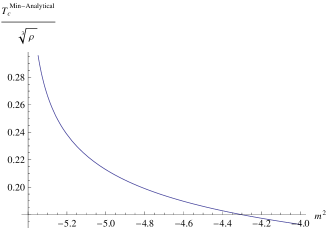
Figure 1: Plot of the $\frac{T_{c}^{Min-Analytical}}{\sqrt[3]{\rho}}$ as a function of the $m^{2}$ for $m_{c}^{2}<m^{2}\leq-4$. The lower and upper BF bounds are $\Big{(}m^{lower}_{BF}\Big{)}^{2}=-4,\ \ \Big{(}m^{upper}_{BF}\Big{)}^{2}=-3$.

We tabulated different values of the critical temperature in Table I. Specially it is interesting that when the mass of the scalar field reaches the BF bound i.e. $m^{2}=m_{BF}^{2}=-4$, the critical temperature $T_{c}$ remains finite. The values of this table are in good agreement with the numerical data plb2011 .

Table 1: Variation of the $\frac{T_{c}}{\sqrt[3]{\rho}}$ as a function of $m^{2}$ for $m_{c}^{2}<m^{2}\leq m_{BF}^{2}$.

$m^{2}=-5.4$	$m^{2}=-5$	$m^{2}=-4.8$	$m^{2}=-4.2$	$m^{2}=m_{BF}^{2}$
0.653067	0.142186	0.124354	0.0988134	0.0938797

III.3 linear relation between $<O_{\Delta}>$ and the chemical potential

In this section we want to obtain the linear relation between $<O_{\Delta}>$ and the chemical potential. For this reason, firstly we rewrite the (9) near the critical point $T\rightarrow T_{c}$, with the solution (11)

$$\phi^{\prime\prime}+s(\xi)\phi^{\prime}=\frac{(\epsilon\xi^{\Delta}\Omega(\xi))^{2}\Big{(}1+c_{4}(\epsilon\xi^{\Delta}\Omega(\xi))^{2}+c_{\alpha}(\epsilon\xi^{\Delta}\Omega(\xi))^{\alpha-2}\Big{)}}{\xi^{2}(1-\xi^{4})(1-24\gamma\xi^{4})}\phi$$ (29)

Here

$$s(\xi)=-\frac{(1+72\gamma\xi^{4})}{\xi(1-24\gamma\xi^{4})}$$

Near the critical point, we must keep only terms of order $\epsilon^{4}$. Since $3<\alpha<4$, thus it’s not necessary to keep all the terms with coefficients. For example now we put $c_{4}\cong 0$, and only we keep the $c_{\alpha}$ term. We write the following approximated solution cai

$$\phi(\xi)\approx\mu_{c}+\epsilon\chi(\xi)$$ (30)

Where $\chi(\xi)$ is a general function, with this auxiliary condition $\chi(0)=1$. the equation for $\chi$ reads

$$\chi^{\prime\prime}(\xi)+s(\xi)\chi^{\prime}(\xi)\approx\mu_{c}\frac{\epsilon(\xi^{\Delta}\Omega(\xi))^{2}\Big{(}1+c_{\alpha}(\epsilon\xi^{\Delta}\Omega(\xi))^{\alpha-2}\Big{)}}{\xi^{2}(1-\xi^{4})(1-24\gamma\xi^{4})}$$ (31)

The solution for $\chi(\xi)$ reads

$$\chi^{\prime}(\xi)=e^{-\int s(\xi)d\xi}(C+\epsilon\int j(\xi)e^{\int s(\xi)d\xi}d\xi)$$ (32)

Where

$$j(\xi)=\mu_{c}\frac{(\xi^{\Delta}\Omega(\xi))^{2}\Big{(}1+c_{\alpha}(\epsilon\xi^{\Delta}\Omega(\xi))^{\alpha-2}\Big{)}}{\xi^{2}(1-\xi^{4})(1-24\gamma\xi^{4})}\\ ,\ \ e^{\int s(\xi)d\xi}=\frac{-1+24\gamma\xi^{4}}{\xi}$$

Now we have

$$\chi^{\prime}(\xi)=\frac{\xi}{24\gamma\xi^{4}-1}(C+\epsilon\int\frac{j(\xi)(24\gamma\xi^{4}-1)}{\xi}d\xi)$$ (33)

Finally we obtain

$$\chi(0)=\frac{\sqrt{6}\pi C}{48\sqrt{\gamma}}$$ (34)

Also, we can expand the $\phi$ near $\xi=0$ as a series solution as the follows

$$\phi\approx\mu-\frac{\rho}{h}\xi^{2}\approx\mu_{c}+\epsilon(\chi(0)+\chi^{\prime}(0)\xi+\frac{1}{2}\chi^{\prime\prime}(0)\xi^{2}+...)$$ (35)

comparing the coefficients of order $\xi^{0}$ we get

$$\mu-\mu_{c}\approx\epsilon\chi(0)$$ (36)

Using (34) we obtain

$$\mu-\mu_{c}\approx\epsilon\Big{(}\frac{\sqrt{6}\pi C}{48\sqrt{\gamma}}\Big{)}$$

Now we obtain

$$\mu-\mu_{c}\approx<O_{\Delta}>\Big{(}\frac{\sqrt{6}\pi C}{48\sqrt{\gamma}}\Big{)}$$

Such linear relation between $<O_{\Delta}>$ and the chemical potential has been discussed previously in s-wave and p-wave superconductors cai .

IV Conclusions

In this paper,we studied the analytical properties of the Stuckelberg holographic superconductors with Weyl corrections, using a variational method. Firstly we reduced the problem to a variational Sturm-Liouville equation near the critical point. We written a suitable functional, and using some trial functions, we obtained the lower bound of the critical temperature $T_{c}$. We showed that, when the expectation value of the dual operators with conformal dimension $\Delta=3$ near the critical point $T=T_{c}$ remain small, we can calculate the $T_{c}$ easily. The expression for $T_{c}$ is a function of the $m^{2}$. We obtained that for positive $T_{c}$, we must have $m^{2}>m_{c}^{2}$. This new lower bound on $m^{2}$ is completely different from the same value of the lower bound obtained from the stability. We discussed the relation between the $T_{c}$ and $m^{2}$. We showed that when $m^{2}$ increases, the $T_{c}$ decreases and the condensation becomes weaker. Further we show that near the BF bound, i.e. when $m^{2}=m^{2}_{BF}$, the $T_{c}$ remains finite. It is shown that there is no divergence near the BF bound for $T_{c}$. Further we obtained that there is a linear relation between $<O_{\Delta}>$ and the chemical potential.

V Acknowledgment

The authors would like to thank Jian Pin Wu (Beijing Normal University-China) , Wen-Yu Wen (Chung Yuan Christian University-Taiwan) and Mubasher Jamil (Center for Advanced Mathematics and Physics -Pakistan) for reading manuscript and helpful discussions and useful comments. We would like to thank anonymous referees for giving useful comments to improve this paper.

References

- (1) J. M. Maldacena, Adv. Theor. Math. Phys. 2, 231 (1998).
- (2) C. P. Herzog, J. Phys. A 42 (2009) 343001 .
- (3) S. A. Hartnoll, Class. Quant. Grav. 26 (2009) 224002.
- (4) G. Policastro, D. T. Son, A. O. Starinets, Phys. Rev. Lett. 87, 081601 (2001).
- (5) P. Kovtun, D. T. Son, A. O. Starinets, JHEP10 (2003) 064.
- (6) S. A. Hartnoll, C. P. Herzog, G. T. Horowitz, JHEP 12 (2008) 015.
- (7) G. T. Horowitz , M. M. Roberts, Phys. Rev. D 78, 126008 (2008).
- (8) R. Gregory, S. Kanno , J. Soda, JHEP10 ,010(2009) .
- (9) Y. Brihaye , B. Hartmann, Phys. Rev. D 81, 126008 (2010).
- (10) R.-G. Cai, Z.-Y. Nie,. H.-Q. Zhang, Phys. Rev. D 82, 066007 (2010).
- (11) Q. Pan , B. Wang, Phys. Lett. B. 693 (2010) 159.
- (12) Q. Pan, J. Jing, B. Wang, JHEP 11 (2011) 088;
- (13) R.-G. Cai , H.-Q. Zhang, Phys. Rev. D81, 066003(2010).
- (14) D. Momeni, M. R. Setare, N. Majd, JHEP 1105 ,118(2011),arXiv:1003.0376 [hep-th].
- (15) E. Nakano, W.-Y. Wen, Phys.Rev.D78,046004(2008).
- (16) D. Momeni, E. Nakano, M. R. Setare, W.-Y. Wen, arXiv:1108.4340v2 [hep-th].
- (17) M. R. Setare, D. Momeni, EPL, 96 (2011) 60006,arXiv:1106.1025.
- (18) Y. Liu, Y. Peng, B. Wang, arXiv:1202.3586 [hep-th].
- (19) Q. Pan, J. Jing, B. Wang, Phys. Rev. D 84, 126020 (2011).
- (20) G. Tallarita, S. Thomas, JHEP 1012:090,2010.
- (21) Q. Pan, J. Jing , B. Wang Phys.Rev. D84, 126020 (2011) .
- (22) Y.-Q. Wang, Y.-X. Liu, R.-G. Cai, S. Takeuchi, H.-Q. Zhang, arXiv:1205.4406 [hep-th].
- (23) S. S. Gubser, S. S. Pufu, JHEP 11 (2008) 033.
- (24) C. P. S. Herzog, S. Pufu, JHEP 0904 (2009) 126.
- (25) M. Ammon , J. Erdmenger , V. Grass, , P. Kerner , A. O’Bannon , Phys. Lett. B 686 ,192(2010) .
- (26) C. P. Herzog, Phys. Rev. D81, 126009 (2010).
- (27) S. Kanno, Class. Quant. Grav. 28, 127001(2011) .
- (28) H.-B. Zeng, X. Gao, Y. Jiang, H.-S. Zong, JHEP 05 (2011) 2.
- (29) Q. Pan, J. Jing , B. Wang , S. Chen ,JHEP, 1206, 087(2012).
- (30) J.-P. Wu, Y. Cao, X.-M. Kuang, W.-J. Li, Phys. Lett. B697, 153 (2011).
- (31) D. Momeni, M.R. Setare, Mod. Phys. Lett. A, 26, 38,2889 (2011), arXiv:1106.0431 .
- (32) J.-P. Wu, arXiv:1006.0456 [hep-th].
- (33) D. Momeni,N. Majd, R. Myrzakulov, EPL, 97 ,61001(2012),arXiv:1204.1246 [hep-th].
- (34) D.-Z. Ma, Y. Cao, J.-P. Wu ,Phys. Lett. B 704, 604(2011) .
- (35) I. T. Drummond , S. J. Hathrell, Phys. Rev. D 22, 343 (1980).
- (36) P. Breitenlohner , D. Z. Freedman, Phys. Lett.B. 115,197 (1982) .
- (37) R.-G. Cai, H.F. Li, H.Q. Zhang, Phys.Rev.D83:126007(2011).