The Smectic $A$ to $C$ Phase Transition in Isotropic Disordered Environments

Abstract

We study theoretically the smectic $A$ to $C$ phase transition in isotropic disordered environments. Surprisingly, we find that, as in the clean smectic $A$ to $C$ phase transition, smectic layer fluctuations do not affect the nature of the transition, in spite of the fact that they are much stronger in the presence of the disorder. As a result, we find that the universality class of the transition is that of the “Random field $XY$ model” ($RFXY$).

The effect of quenched disorder on condensed matter systems has been widely studied for many yearsHarris ; Geoff ; Aharony , both for practical reasons (since disorder is always present in real systems) and fundamental ones. Disorder can destroy many types of long ranged order (e.g., ferromagnetic order in systems with quenched random fields RFferro ), and it can radically change the critical behavior of many phase transitionsAharony .

Such effects have been found in, e.g., superconductorsSC , charge density wavesCDW ; CDWRT , Josephson junction arraysJJunc , superfluid helium in aerogelHelium , and ferromagnetic superconductorsSCferro .

Some of the most novel and dramatic effects of quenched disorder are found in liquid crystals confined in random porous mediaLC ; RT . These intriguing systems exhibit a variety of exotic “Bragg Glass” phases. They also undergo unique types of phase transitionsCT , one of which, the Smectic $A$ to Smectic $C$ (hereafter, $AC$) transitionGP ; ACexp , is the subject of this paper.

In the high temperature phase (the “$A$” phase), the nematic director $\hat{n}$ (which points along the axis of alignment of the constituent long molecules that make up the smectic material), and the normal $\hat{N}$ to the smectic layers , are parallel. In the low temperature phase (the “$C$” phase), $\hat{n}$ and $\hat{N}$ tilt away from each other.

The $AC$ transition in clean systems was first considered by deGennesdeGennesAC , who showed that, if fluctuations of the smectic layers could be neglected, the $AC$ transition should be in the universality class of the ferromagnetic $XY$ modelLubensky .

The effect of layer fluctuations on this result was considered later by Grinstein and Pelcovits GP , who showed that their effect on the $AC$ transition can, in fact, be neglected, and that, therefore, the $AC$ transition in clean systems is $XY$-like.

Unfortunately, for reasons not yet well understood, the critical region of the $AC$ transition in clean systems appears to be extremely small; as a result, most experimental systems exhibit a transition that is accurately described by mean-field theoryMF . As a result, no definitive experimental test of the above predictions has yet been made.

Recently the nature of the $AC$ transition has been studied for a liquid crystal confined in uniaxialCT and biaxialCT2 disordered environments. In these systems, the anisotropy essentially freezes the direction of the molecular axes, and the $AC$ transition can be described entirely in terms of the configuration of the smectic layers CT ; CT2 .

In an isotropic quenched random environment (which can be realized most simply by putting the smectic in aerogelBirAC ), which we study in this paper, the problem is in many ways more difficult, since now both fluctuations of the molecular direction and those of the layers must be addressed. Indeed, it is not even obvious that the two phases between which the transition we wish to study occurs even exist in $d=3$; the stability of the $A$ phase in the presence of even arbitrarily weak disorder remains an open question both theoreticallyRT , and experimentallyLC . Presumably, similar issues arise with the $C$ phase.

However, if we assume that both the $A$ and $C$ phases are stable, then we are able to completely determine the nature of the transition between them. We find that, if this stability assumption is correct, the layer fluctuations do not affect the universality class of this transition, which proves to be just that of the random field $XY$ modeld->d-2 ; Dan Fisher RFXY .

This implies a substantial quantitative change in the universal critical exponents from their values in the clean problem. It is knownd->d-2 that the coefficients in the $\epsilon=6-d$ expansion for the critical exponents of the random field $XY$ model are exactly the same as those for the $\epsilon=4-d$ expansion of the clean (i.e., no random field) problem. However, since $\epsilon=3$ in the physical case $d=3$ for the random field problem, the $\epsilon$-expansion is not quantitatively reliable. It is clear, however, that the exponents will be quite different from those for the clean $XY$ model, as even the first order in $\epsilon$ terms change by a factor of 3.

From a quantitative standpoint, the most useful feature of our result is that it connects the exponents of the $AC$ transition in an isotropic disordered environment to those of a random field $XY$ model, as can be experimentally realized in, e.g., anti-ferromagnets with substitutional disorderbirgRF .

The remainder of this paper is devoted to demonstrating that the $AC$ transition in the presence of isotropic disorder is in the random field $XY$ universality class.

Our starting model is a modification of the model for clean smectics near a Smectic A-Smectic C transitionGP , the Hamiltonian $H=H_{u}+H_{c}+H_{uc}$ for which consists of three parts:

$$H_{u} = {1\over 2}\int d^{d}r\left[K(\nabla^{2}_{\perp}u)^{2}+B\left(\partial_{z}u-{1\over 2}\left|\vec{\nabla}u\right|^{2}\right)^{2}\right],$$

$$H_{c} = {1\over 2}\int d^{d}r\left[K_{1}\left(\vec{\nabla}\cdot\vec{c}\right)^{2}+K_{2}\left(\vec{\nabla}\times\vec{c}\right)^{2}\right.$$

$$\left.+K_{3}\left(\partial\vec{c}\over\partial z\right)^{2}+Dc^{2}+2vc^{4}\right],$$

$$H_{uc} = {1\over 2}\int d^{d}r\left[g_{1}c^{2}\left(\partial_{z}u-{1\over 2}|\vec{\nabla}u|^{2}\right)+g_{2}(\nabla_{\perp}^{2}u)\times\right.$$

$$\left.(\vec{\nabla}\cdot\vec{c})+g_{3}\left(\partial\vec{c}\over\partial z\right)\cdot\left(\partial_{z}\vec{\nabla}_{\perp}u\right)+D(\vec{c}\cdot\vec{\nabla}_{\perp}u)^{2}\right],$$

where we have defined the direction parallel to the averaged layer normal in the $A$ phase as the $\hat{z}$-axis, and the plane perpendicular to $\hat{z}$ as $\perp$. Here $\vec{c}$, which is roughly the projection of $\hat{n}$ onto the layers, is the order parameter for the transition. More precisely, it has only two non-zero components (i.e., $c_{z}(\vec{r})=0$), given by

$$c^{\perp}_{i}(\vec{r}) = \left[\delta_{ij}-N_{i}(\vec{r})N_{j}(\vec{r})\right]n_{j}(\vec{r}),\ \ i\in\perp,$$ (1)

where $\hat{N}(\vec{r})$ denotes the unit vector along the layer normal, given by $\hat{N}={\hat{z}-\vec{\nabla}u\over\mid\hat{z}-\vec{\nabla}u\mid}$. Note that all terms in the Hamiltonian are rotation invariant. This is because the environment is isotropic and rotating the smectic does not cost energy. The pieces $H_{u}$ and $H_{c}$ are, respectively, just the elastic energies for smectic layer fluctuations and molecular reorientations, while $H_{uc}$ couples $u$ and $\vec{c}$.

The fourth term in $H_{c}$ and the last term in $H_{uc}$ , which come from a term $D(T)\mid\hat{N}-\hat{n}\mid^{2}$, induce the $AC$ transition via a sign change in the temperature $T$-dependent coefficient $D(T)$. For $T>T_{AC}$, $D>0$, and the free energy is minimized at $\vec{c}=\vec{0}$, so the system is in the $A$ phase. For $T<T_{AC}$, $D<0$, and the free energy is minimized at $\vec{c}\neq\vec{0}$, so the system is in the $C$ phase.

Now we include disorder. The aerogel exerts a variety of random forces on the molecular axes and the smectic layersRT ; CT ; the most important of them areRT ; CT the “random tilt fields”, which tend to align the local molecules and the local normals with the random aerogel strands. The contribution of these random effects to the free energy can be written asRT ; CT

$$\int d^{d}r\left[\vec{h}(\vec{r})\cdot\vec{\nabla}_{\perp}u+\vec{h}^{c}(\vec{r})\cdot\vec{c}\right],$$ (2)

where the quenched random fields $\vec{h}(\vec{r})$ and $\vec{h}^{c}(\vec{r})$ are taken to have Gaussian distributions of zero mean, with anisotropic short-ranged correlations:

$$\overline{h_{i}(\vec{r})h_{j}(\vec{r}\,^{\prime})}=\Delta\delta^{\perp}_{ij}\delta^{d}(\vec{r}-\vec{r}\,^{\prime}),$$ (3)

$$\overline{h^{c}_{i}(\vec{r})h^{c}_{j}(\vec{r}\,^{\prime})}=\Delta_{c}\delta^{\perp}_{ij}\delta^{d}(\vec{r}-\vec{r}\,^{\prime}),$$ (4)

$$\overline{h^{c}_{i}(\vec{r})h_{j}(\vec{r}\,^{\prime})}=\Delta^{\prime}\delta^{\perp}_{ij}\delta^{d}(\vec{r}-\vec{r}\,^{\prime}).$$ (5)

The first term in equation (2) has been treated in the earlier workRT on the smectic $A$ phase in isotropic disordered environments, where it leads to strong power-law anomalousRT . The second term is just the random field disorder present in the $RFXY$ modelRFferro ; Dan Fisher RFXY .

To cope with the quenched disorder we employ the replica trick Geoff . We assume that the free energy of the system for a specific realization of the disorder is the same as that averaged over many realizations. To calculate the averaged free energy $\overline{F}=\overline{\ln{Z}}$, where $Z$ is the partition function, we use the mathematical identity $\ln{Z}=\lim_{n\to 0}{Z^{n}-1\over n}$. When calculating $\overline{Z^{n}}$, we can first compute the average over the random fields $\vec{h}(\vec{r})$, whose statistics have been given earlier. Implementing this procedure gives a replicated Hamiltonian $H^{r}=H^{r}_{u}+H^{r}_{c}+H^{r}_{uc}$ with the effect of the random fields transformed into couplings between $n$ replicated fields, with the limit $n\rightarrow 0$ corresponding to the original quenched disorder problem:

$$H_{u}^{r} = {1\over 2}\int d^{d}r\sum_{\alpha=1}^{n}\left[B\left(\partial_{z}u_{\alpha}-{1\over 2}\left|\vec{\nabla}u_{\alpha}\right|^{2}\right)^{2}\right.$$

$$\left.+K(\nabla^{2}_{\perp}u_{\alpha})^{2}\right]-{\Delta\over 2k_{B}T}\int d^{d}r\sum_{\alpha,\beta=1}^{n}\vec{\nabla}_{\perp}u_{\alpha}\cdot\vec{\nabla}_{\perp}u_{\beta},$$

$$H_{c}^{r} = {1\over 2}\int d^{d}r\sum_{\alpha=1}^{n}\left[K_{1}\left(\vec{\nabla}\cdot\vec{c}_{\alpha}\right)^{2}+K_{2}\left(\vec{\nabla}_{\perp}\times\vec{c}_{\alpha}\right)^{2}\right.$$ (7)

$$\left.+K_{3}\left(\partial\vec{c}_{\alpha}\over\partial z\right)^{2}+Dc_{\alpha}^{2}+2vc_{\alpha}^{4}\right]$$

$$-{\Delta_{c}\over 2k_{B}T}\int d^{d}r\sum_{\alpha,\beta=1}^{n}\vec{c}_{\alpha}\cdot\vec{c}_{\beta},$$

$$H_{uc}^{r} = {1\over 2}\int d^{d}r\left[\sum_{\alpha=1}^{n}\left(g_{1}c_{\alpha}^{2}\left(\partial_{z}u_{\alpha}-{1\over 2}|\vec{\nabla}u_{\alpha}|^{2}\right)\right.\right.$$ (8)

$$\left.\left.+g_{2}(\nabla_{\perp}^{2}u_{\alpha})(\vec{\nabla}\cdot\vec{c}_{\alpha})+g_{3}\left(\partial\vec{c}_{\alpha}\over\partial z\right)\cdot\left(\partial_{z}\vec{\nabla}_{\perp}u_{\alpha}\right)\right.\right.$$

$$\left.\left.+D(\vec{c}_{\alpha}\cdot\vec{\nabla}_{\perp}u_{\alpha})^{2}\right)\right].$$

If we set $u_{\alpha}=0$, the entire Hamiltonian reduces to Eq. (7), which reduces to the $RFXY$ model if $K_{1}=K_{2}=K_{3}$. An RG analysis shows that departures from this “one constant approximation” (i.e., $K_{1,2,3}=K$) are irrelevantfoot3 ; hence, in the absence of the $u$ field, the transition is in the $RFXY$ universality class.

The piece $H_{u}^{r}$ Eq. (LABEL:Hur) of $H$ which involves $u$ alone is precisely the model for smectics $A$ in isotropic aerogel studied in referenceRT . From the analysis of that reference, we know that the critical dimension of Eq. (LABEL:Hur), below which the anharmonic terms in Eq. (LABEL:Hur) become important, is $5$. On the other hand, the critical dimension of $H_{c}^{r}$ Eq. (7) is well knownRFferro ; Dan Fisher RFXY ; d->d-2 to be $6$. Because of this discrepancy between the two critical dimensions, a standard $\epsilon$-expansion study of the entire model Eqs. (LABEL:Hur-8)” is impossible. Our solution to this quandry is to integrate out only the $u_{\alpha}$ fields perturbatively in a momentum shell RG approach, which is controlled in an $\epsilon=5-d$-expansion, to obtain an effective model that only involves $\vec{c}_{\alpha}$. While unorthodox, this approach is very much in the spirit of more conventional RG’s: we are performing a partial trace over some degrees of freedom to obtain a more tractable Hamiltonian in terms of the degrees of freedom remaining after the trace.

The momentum shell RG procedure consists of tracing over the short wavelength Fourier modes of $u_{\alpha}(\vec{r})$ followed by a rescaling of the length. We initially restrict wavevectors to lie in a bounded Brillouin zone which we take to be the infinite cylinder $0<\mid\vec{q}_{\perp}\mid<\Lambda$, $-\infty<q_{z}<\infty$, where $\Lambda\sim 1/a$ is an ultra-violet cutoff, and $a$ is the smectic layer spacing. The displacement field $u_{\alpha}(\vec{r})$ is separated into high and low wave vector parts $u_{\alpha}(\vec{r})=u_{\alpha}^{<}(\vec{r})+u_{\alpha}^{>}(\vec{r})$, where $u_{\alpha}^{>}(\vec{r})$ has support in the thin wave vector shell $\Lambda e^{-d\ell}<\mid\vec{q}_{\perp}\mid<\Lambda$, $-\infty<q_{z}<\infty$. Here $d\ell$ is a differential parameter $d\ell\ll 1$. We first integrate out $u^{>}_{\alpha}(\vec{r})$. This integration is done perturbatively in the anharmonic terms in $H$ Eqns. (LABEL:Hur)-(8). After this perturbative step, we anisotropically rescale lengths, with $\vec{r}_{\perp}=\vec{r}^{~{}\prime}_{\perp}e^{\ell}$, $r_{z}=r^{\prime}_{z}e^{\omega\ell}$, so as to restore the UV cutoff back to $\Lambda$. This is then followed by rescaling the long wave length part of the field with $u_{\alpha}^{<}(\vec{r})=u^{\prime}_{\alpha}(\vec{r^{\prime}})e^{\chi\ell}$. The underlying rotational invariance insures that the graphical corrections preserve the rotationally invariant operator $\partial_{z}u_{\alpha}-{1\over 2}\left(\vec{\nabla}u_{\alpha}\right)^{2}$ renormalizing it as a whole. It is therefore convenient to choose the dimensional rescaling that also preserves this operator, which is $\chi=2-\omega$.

After this procedure we obtain the following RG flow equations to one-loop order, ignoring the term $D\left(\vec{c}_{\alpha}\cdot\vec{\nabla}_{\perp}u_{\alpha}\right)^{2}$, since we are interested in the critical point where $D$ vanishes:

$${dB\over d\ell} = \left(d+3-3\omega-{3\over 16}g\right)B,$$ (9)

$${dK\over d\ell} = \left(d-1-\omega+{1\over 32}g\right)K,$$ (10)

$${d\Delta\over d\ell} = \left(d+1-\omega+{1\over 64}g\right)\Delta,$$ (11)

$${dg_{1}\over d\ell} = \left(d+1-\omega-{3\over 16}g\right)g_{1},$$ (12)

$${dv\over d\ell} = \left(d-1+\omega-{3g\over 128}{g_{1}^{2}\over Bv}\right)v.$$ (13)

where $g$ is a dimensionless coupling:

$$g\equiv\Delta\left(B\over K^{5}\right)^{1\over 2}C_{d-1}\Lambda^{d-5},$$ (14)

where $C_{d}$ is the surface area of a $d$-dimensional sphere with radius one divided by $(2\pi)^{d}$.

Note that the graphical corrections inside the parenthesis in Eqs. (9) and (12) are the same. This is not just an an approximation to one-loop order, but exact to arbitrary loop order. This can be easily understood by analyzing the structures of the Feynman graphs. In Fig. 1 the upper graph summaries all the possible graphical corrections to $(\partial_{z}u_{\alpha})\mid\vec{\nabla}_{\perp}u_{\alpha}\mid^{2}$; the lower one does for $(\partial_{z}u_{\alpha})c_{\alpha}^{2}$. The parts inside the two square boxes are the same no matter how complicated they are and how many loops they have.

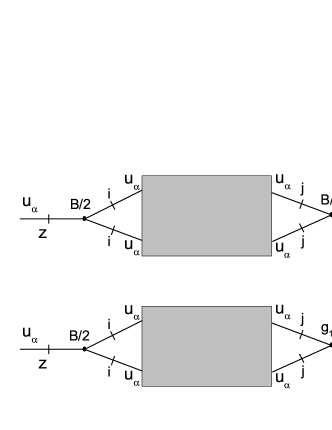
Figure 1: Schematic representation of all Feynman graphs that renormalize $B$ (top diagram) and $g_{1}$ (bottom diagram). In each case the gray box represents all possible ways of connecting the portions of the Feynman graphs shown. These are identical for both graphs; as a result, the graphical corrections to $B$ and $g_{1}$ obey $(dB/dl)_{graph}=(dg_{1}/dl)_{graph}(g_{1}/B)$. This in turn implies that the anomalous elasticity for $g_{1}$ (see text) is identical, up to a multiplicative constant, to that for $B$.

There are no graphical corrections to $(\nabla_{\perp}^{2}u_{\alpha})(\vec{\nabla}\cdot\vec{c}_{\alpha})$, which is also exact to arbitrary-loop order. This is because both terms have one power of $c_{\alpha}$ while all anharmonic terms have even powers of $c_{\alpha}$. Therefore, under renormalization both $g_{2,3}$ flow only as a result of length and field rescaling.

The recursion relations for $B$, $K$, and $\Delta$ are identical with those found for a smectic $A$ in an isotropic disordered medium in referenceRT . This is also exact to all orders, since we have not, in our unusual approach, integrated out the $\vec{c}$ fluctuations. This means that all of the results obtained in RT for the long-wavelength behavior of these quantities also hold here. We will also make use of this fact later.

To analyze these flow equations we introduce an additional dimensionless coupling: $g_{3}\equiv{g_{1}^{2}\over Bv}$. Combining flow Eqs. (9-13) with the definitions of $g$ and $g_{3}$ we find

$${dg\over d\ell} = \epsilon g-{5\over 32}g^{2},$$ (15)

$${dg_{3}\over d\ell} = {3g\over 128}\left(-8+g_{3}\right)g_{3},$$ (16)

where $\epsilon=5-d$. These flow equations have four fixed points: $g^{*}=0\ \ \mbox{or}\ \ {32\over 5}\epsilon,g_{3}^{*}=0\ \ \mbox{or}\ \ 8$. The RG flows of $g$ and $g_{3}$ around these fixed points are illustrated in Fig. 2. Note that $g_{3}^{*}=8$ corresponds to the stability limit of the system. Linearizing Eqs. (15, 16) around the only stable fixed point $g^{*}={32\over 5}\epsilon$, $g_{3}^{*}=0$, we find the graphical corrections to $v$ vanish exponentially as $\ell\to\infty$. This implies that integrating out $u_{\alpha}$ only gives a finite correction to $v$, even at arbitrarily long wavelengths. Hence, these corrections to $v$ coming from the $u_{\alpha}$ fields do not affect the nature of the $AC$ transition.

Figure 2: RG flows of the dimensionless couplings $g$ and $g_{3}$ from equations (15) and (16). All initial models starting to the left of the stability limit $g_{3}=8$ flow into the $g=g^{*}$, $g_{3}=0$ fixed point, which therefore controls the $AC$ transition. All models starting to the right of the stability limit are unstable.

During each RG cycle the integration over $u_{\alpha}^{>}$ also generates terms which do not exist in $H_{c}^{r}$. The most relevant ones are produced in the second cumulant by $(\partial_{z}u_{\alpha})c_{\alpha}^{2}$ and $(\nabla_{\perp}^{2}u_{\alpha})(\vec{\nabla}\cdot\vec{c}_{\alpha})$. Elementary power counting shows that the terms generated by $\left(\partial\vec{c}_{\alpha}\over\partial z\right)\cdot\left(\partial_{z}\vec{\nabla}_{\perp}u_{\alpha}\right)$ are less relevant.

We’ll now show that these terms also do not affect the nature of the $AC$ transition. We start with the terms generated by $(\partial_{z}u_{\alpha})c_{\alpha}^{2}$:

$$\sum_{\alpha,\beta}^{n}\sum_{\vec{q}_{1,2}\vec{k}}g_{1}^{2}(\vec{k})\left[{k_{B}Tk_{z}^{2}G(\vec{k})}\delta_{\alpha\beta}+{\Delta(\vec{k})k_{z}^{2}k_{\perp}^{2}G^{2}(\vec{k})}\right]$$

$$\times c_{\alpha,i}(\vec{q}_{1})c_{\alpha,i}(-\vec{q}_{1}+\vec{k})c_{\beta,i}(\vec{q}_{2})c_{\beta,i}(-\vec{q}_{2}-\vec{k})$$ (17)

where $G(\vec{k})\equiv 1/[B(\vec{k})k_{z}^{2}+K(\vec{k})k_{\perp}^{4}]$. The $\vec{k}$-dependences of $B$, $K$, $\Delta$, and $g_{1}$ arise due to the the nonzero graphical corrections in the recursion relations Eqs. (9-12). Because, as mentioned earlier, Eqs. (9-11) are identical, to all orders, with those for a smectic $A$ in an isotropic disordered environment, we can simply use the results of RT for the wavevector dependences of these quantities. Furthermore, since, as noted earlier, there is an exact relation between the renormalization of $g_{1}$ and that of $B$, the wavevector dependence of $g_{1}$ is identical to that of $B$, up to an overall multiplicative constant.

Using the just noted connections to the work of RT , we can simply quote $\vec{k}$-dependences of $B$, $K$, $\Delta$, and $g_{1}$:

$$B(\vec{k}),g_{1}(\vec{k})\propto\left\{\begin{array}[]{ll}k_{\perp}^{\eta_{B}},&k_{z}\ll k_{\perp}^{\zeta},\\ k_{z}^{\eta_{B}/\zeta},&k_{z}\gg k_{\perp}^{\zeta},\end{array}\right.$$ (20)

$$K(\vec{k}),\Delta(\vec{k})\propto\left\{\begin{array}[]{ll}k_{\perp}^{-\eta_{K,\Delta}},&k_{z}\ll k_{\perp}^{\zeta},\\ k_{z}^{-\eta_{K,\Delta}/\zeta},&k_{z}\gg k_{\perp}^{\zeta},\end{array}\right.$$ (23)

where the anisotropy scaling exponent $\zeta=2-{{\eta_{B}+\eta_{K}}\over 2}$, and $\eta_{B,K,\Delta}>0$. Another result of RT is that the exponents $\eta_{B,K,\Delta}$ are not fully independent, but connected by the exact scaling relation:

$$5-d+\eta_{\Delta}={\eta_{B}\over 2}+{5\over 2}\eta_{K},$$ (24)

which is implied by the fact that $g$ flows to a nonzero stable fixed point RT . Furthermore, there are certain bonds on the values of $\eta_{B,K}$ that must be satisfied in order for the smectic $A$ phase in an isotropic random environment to be stable, which is a prerequisite condition for the existence of a sharp smectic $A$-$C$ transition RT in such environments. It is only meaningful within these bounds to discuss the relevance of the terms in formula (17). These bounds are

$$\eta_{K}+\eta_{B}<2,~{}~{}\eta_{K}<1,~{}~{}\eta_{B}+5\eta_{K}>4.$$ (25)

The first two bounds come from the requirement of long-ranged orientational order and the condition for dislocations to remain confined, respectively. The third bound is obtained by combining $\eta_{\Delta}>0$ with the exact scaling relation (24) in $d=3$.

Using expressions (20, 23) we can write equation (17) in a scaling form:

$$\sum_{\alpha,\beta}^{n}\sum_{\vec{q}_{1,2}\vec{k}}\left[k_{\perp}^{\eta_{B}}f_{1}\left(k_{z}\over k_{\perp}^{\zeta}\right)\delta_{\alpha\beta}+k_{\perp}^{(\eta_{B}-3\eta_{K})/2}f_{2}\left(k_{z}\over k_{\perp}^{\zeta}\right)\right]$$

$$\times c_{\alpha,i}(\vec{q}_{1})c_{\alpha,i}(-\vec{q}_{1}+\vec{k})c_{\beta,i}(\vec{q}_{2})c_{\beta,i}(-\vec{q}_{2}-\vec{k}),~{}~{}~{}$$ (26)

where $f_{1,2}(x)$ are scaling functions. Clearly, as $\vec{k}\to\vec{0}$ the replica-diagonal term (i.e., the one which contains $\delta_{\alpha\beta}$) in (26) is irrelevant compared to the quartic ($v$) term in $H_{c}^{r}$, since its coefficient vanishes like $k_{\perp}^{\eta_{B}}$.

To decide whether the off-diagonal piece is relevant, we treat it as a perturbation and calculate its contributions to $D$:

$$\delta D = \int d^{d}k\ \ k_{\perp}^{(\eta_{B}-3\eta_{K})/2}f_{2}\left(k_{z}\over k_{\perp}^{\zeta}\right){1\over ck^{2}+D}$$

$$= \int d^{d}k\ \ k_{\perp}^{(\eta_{B}-3\eta_{K})/2}f_{2}\left(k_{z}\over k_{\perp}^{\zeta}\right){1\over ck^{2}}\left(1-{D\over ck^{2}}\right).$$

It is readily shown that this integral converges for $d$ near $6$ if the exponents $\eta_{B,K}$ satisfy the bounds (25). Therefore, this off-diagonal piece is also irrelevant.

Now we discuss the terms generated by $(\nabla_{\perp}^{2}u_{\alpha})(\vec{\nabla}\cdot\vec{c}_{\alpha})$, which also have a diagonal and an off-diagonal part:

$$\sum_{\alpha,\beta}^{n}\sum_{\vec{q}} g_{2}^{2}\left[k_{B}T{q_{\perp}^{4}G(\vec{q})}\delta_{\alpha\beta}+{\Delta(\vec{q})q_{\perp}^{6}G^{2}(\vec{q})}\right]\times$$ (27)

$$q_{i}q_{j}c_{\alpha,i}(\vec{q})c_{\beta,j}(-\vec{q}).$$

Here, unlike $g_{1}$, $g_{2}$ has no dependence on $\vec{q}$ since there are no graphical corrections to $(\nabla_{\perp}^{2}u_{\alpha})(\vec{\nabla}\cdot\vec{c}_{\alpha})$. Again we can rewrite Eq. (27) in a scaling form:

$$\sum_{\alpha,\beta}^{n}\sum_{\vec{q}} g_{2}^{2}\left[q_{\perp}^{\eta_{K}}f_{3}\left(q_{z}\over q_{\perp}^{\zeta}\right)\delta_{\alpha\beta}+q_{\perp}^{-\left(\eta_{B}+3\eta_{K}\right)/2}f_{4}\left(q_{z}\over q_{\perp}^{\zeta}\right)\right]$$ (28)

$$\times q_{i}q_{j}c_{\alpha,i}(\vec{q})c_{\beta,j}(-\vec{q}),$$

where $f_{3,4}(x)$ are scaling functions similar to $f_{1,2}(x)$. Clearly, both terms are subdominant to the quadratic terms in $H_{c}^{r}$ as $q\to 0$ provided that $\eta_{B,K}$ are within the stability bounds.

Therefore, we conclude that integrating out $u_{\alpha}$ only gives minor corrections to $H_{c}^{r}$, which do not affect the nature of the transition. Therefore, the universality class of the transition is just that of the random field $XY$ model, as it would be were the full Hamiltonian just $H_{c}^{r}$.

In summary, in this paper we’ve studied the smectic $A$ to $C$ phase transition in isotropic disordered environment. Our analysis shows that if the smectic phases are stable against fluctuations and unbinding of dislocations, the universality class of the transition is that of the “Random Field $XY$ Model”. Surprisingly, in spite of the fact that the smectic layer fluctuations are large due to the disorder, they have no effect on the nature of the transition; that is, if the layers can be frozen by some experimental means the universality class of the transition still remains the same. During this study we developed a“partial renormalization group” strategy which proves to be very successful. We expect this strategy to be useful in dealing with many problems with anharmonic Hamiltonians which involve multiple fields with different critical dimensions.

We thank G. Grinstein for valuable discussions, and for leading JT to the ice cream place under the Brooklyn Bridge. We’re both also grateful to the MPIPKS, Dresden, where a portion of this work was done, for their support (financial and otherwise) and hospitality. JT thanks the U.S. National Science Foundation for their financial support through awards # EF-1137815 and 1006171; LC acknowledges support by the National Science Foundation of China (under Grant No. 11004241) and the Fundamental Research Funds for the Central Universities (under Grant No. 2010LKWL09). LC also thanks the China Scholarship Fund for supporting his visit to the University of Oregon, where a portion of this work was done. He is also grateful to the University of Oregon’s Physics Department and Institute for Theoretical Science for their hospitality.

References

- (1) A.B. Harris, J. Phys. C 7, 1671 (1974).
- (2) G. Grinstein and A. H. Luther, Phys. Rev. B 13, 1329 (1976).
- (3) A. Aharony in Multicritical Phenomena, edited by R. Pynn and A. Skjeltorp (Plenum, New York, 1984), p. 309.
- (4) Y. Imry and S. Ma, Phys. Rev. Lett. 35, 1399 (1975).
- (5) See, e.g., D. S. Fisher, M. P. A. Fisher, and D. A. Ḣuse, Phys. Rev. B. 43, 130 (1991); C. Ebner and D. Stroud, ibid. 31, 165 (1985); D. A. Huse and H. S. Seung, ibid. 42, 1059(1990).
- (6) See, e.g., Charge Density Waves in Solids, edited by L. P. Gorkov and G. Gruner (Elsevier, Amsterdam, 1989);.
- (7) Disorder effects can actually be exploited to make a novel “current effect transistor”; see: L. Radzihovsky and J. Toner, Phys. Rev. Lett. 81, 3711 (1998), for the theoretical prediction; and N. Markovic, M. A. H. Dohmen, and H. S. J. van der Zant, Phys. Rev. Lett. 84, 534 (2000) , for the experimental confirmation.
- (8) See, e.g., E. Granato and J. M. Kosterlitz, Phys. Rev. B. 33, 6533 (1986); Phys. Rev. Lett. 62, 823 (1989).
- (9) See, e.g., M. Chan et al., Phys. Today 49, No. 8, 30 (1996).
- (10) See, e.g., L. Radzihovsky, A. M. Ettouhami, K. Saunders, and J. Toner, Phys. Rev. Lett. 87, 027001 (2001); K. Saunders, L. Radzihovsky and J. Toner, Phys. Rev. Lett. 85, 4309 (2000).
- (11) T. Bellini, L. Radzihovsky, J. Toner, and N. Clark, Science, 294, 1074 (2001); P. S. Clegg, R. J. Birgeneau, S. Park, C. W. Garland, G. S. Iannacchione, R. L. Leheny and M. E. Neubert; Phys. Rev. E, 68, 031706 (2003); R. Guégan, D. Morineau, C. Loverdo, W. Béziel and M. Guendouz, ibid. 73, 011707 (2006), D. Liang and R. L. Leheny, ibid. 75, 031705 (2007); .
- (12) L. Radzihovsky and J. Toner, Phys. Rev. Lett. 78, 23 (1997); Phys. Rev. B. 60, 206 (1999).
- (13) L. Chen and J. Toner, Phys. Rev. Lett. 94, 137803 (2005); Phys. Rev. E. 79, 031703 (2009); ibid. 85, 031703 (2012).
- (14) See, e.g., G. Grinstein and R. A. Pelcovits, Phys. Rev. A. 26, 2196 (1982).
- (15) See, e.g., H. Y. Liu, C. C. Huang, Ch. Bahr, and G. Heppke, Phys. Rev. Lett. 61, 345 (1988).
- (16) P. G. de Gennes, C. R. Acad. Sci. 274, 758 (1972); Mol. Cryst. Liq. Cryst. 21, 49 (1973).
- (17) See, e.g., P. M. Chaikin and T. C. Lubensky, Principles of Condensed Matter Physics, (University Press, Cambridge, 2001).
- (18) P. M. Johnson, C. C. Huang, E. Gorecka, and D. Pociecha, Phys. Rev. E 58, R1207 (1998); C. R. Safinya, M. Kaplan, J. Als-Nielsen, R. J. Birgeneau, D. Davidov, J. D. Litster, D. L. Johnson, and M. Neubert, Phys. Rev. B 21, 4149 (1980); C. C. Huang and J. Viner, Phys. Rev. A 25, 3385 (1982); C. C. Huang and S. C. Lien, ibid.31, 2621 (1985); F. Yang, G. W. Bradberry, and J. R. Sambles, Phys. Rev. E 50, 2834 (1994); I. Musevic, M. Skarabot, R. Blinc, W. Schranz, and P. Dolinar, Liq. Cryst. 20, 771 (1996), and references therein.
- (19) L. Chen and J. Toner, Phys. Rev. E 85, 031703 (2012).
- (20) See, e.g., G. Cordoyiannis, G. Nounesis, V. Bobnar, S. Kralj, and Z. Kutnjak, Phys. Rev. Lett. 94, 027801 (2005); and B. Freelon, M. Ramazanoglu, P. J. Chung, R. N. Page, Yuan-Tse Lo, P. Valdivia, C. W. Garland, and R. J. Birgeneau, Phys. Rev. E 84, 031705 (2011).
- (21) A. Aharony, Y. Imry, and S.-k. Ma, Phys. Rev. Lett. 37, 1364 (1976).
- (22) D. S. Fisher, Phys. Rev. Lett. 78, 1964 (1997).
- (23) H. Yoshizawa, R. A. Cowley, G. Shirane, R. J. Birgeneau, H. J. Guggenheim, and H. Ikeda, Phys. Rev. Lett. 48, 438 (1982).
- (24) The RG analysis is similar to the pure case GP . We find that, in an expansion, the eigenvalue of this perturbation is , where denotes the number of components of .