Exact solution of two friendly walks above a sticky wall with single and double interactions

Abstract

We find, and analyse, the exact solution of two friendly directed walks, modelling polymers, which interact with a wall via contact interactions. We specifically consider two walks that begin and end together so as to imitate a polygon. We examine a general model in which a separate interaction parameter is assigned to configurations where both polymers touch the wall simultaneously, and investigate the effect this parameter has on the integrability of the problem. We find an exact solution of the generating function of the model, and provide a full analysis of the phase diagram that admits three phases with one first-order and two second-order transition lines between these phases. We argue that one physically realisable model would see two phase transitions as the temperature is lowered.

1 Introduction

The adsorption of polymers on a sticky wall, and confined between two walls, has been the subject of continued interest [1, 2, 3, 4, 5, 6, 7, 8, 9, 10, 11, 12]. This has been in part due to the advent of experimental techniques able to micro-manipulate single polymers [13, 14, 15] and the connection to modelling DNA denaturation [16, 17, 18, 19, 20, 21, 22, 23].

Consider a polymer in a dilute solution of good solvent, so that it is in a swollen state [24]. If such a polymer is then attached to a wall at one end the rest of the polymer drifts away due to entropic repulsion. On the other hand, if the wall has an attractive contact potential, so that it becomes ‘sticky’ to the monomers, the polymer can be made to stay close to the wall by a sufficiently strong potential, or for low enough temperatures. The phase transition between these two states is the adsorption transition. The high temperature state is desorbed while the low temperature state is adsorbed. This pure adsorption transition has been well studied [1, 2, 25, 3, 26] exactly and numerically, and has been demonstrated to be second-order.

There has been recent interest [9] in ring polymers, modelled by self-avoiding polygons, being adsorbed onto the walls of a two-dimensional slit. In that work, models in which both sides of the polygon could interact with each of the walls were considered. This provides us with one of the motivations for the model here, where we consider two directed walks that begin and end together, so forming a polygon. We consider directed walks because they often admit exact solutions, while the more realistic self-avoiding walks do not. Moreover, we consider such a pair of walks interacting with a sticky wall, allowing different interactions when one or both walks are near the wall. To allow for a simple realisation of the model we consider so-called friendly directed walks (rather than the ubiquitous vicious walks) where the two walks may share edges of the lattice. However, we do not allow the walks to cross and so there is always an upper walk/polymer and a lower walk/polymer.

Other physical motivations for two-walk models have appeared in the literature. In particular, one may model DNA-denaturation in this way — for example the Poland-Scheraga models [27, 28]. It would be interesting to see if the techniques described below could be used to find exact solutions of the DNA unzipping transition in the presence of an adsorbing wall, such as that discussed in [29]. To do so we would add a contact interaction between the two walks, rather than the double-visit interaction discussed here. A manuscript on this topic is in preparation [30].

As we investigated the model another motivation for its interest became apparent; the full two parameter model is not amenable to one of the standard methods of solving multiple walk models. The Lindström-Gessel-Viennot lemma [31, 32] (which was also considered earlier in a probabilistic context by Karlin and McGregor [33]) decomposes the solution of models of multiple vicious walks into combinations of single walk problems. The lemma implies that the generating function of a multiple walk model would be governed by a D-finite (Differentiably-Finite) function, but the solution of our model is not D-finite. Despite this, we are still able to solve the model.

We have solved our model in two ways. Firstly, we use the obstinate kernel method (see [34] for an overview of the technique) to give a formal solution of a functional equation as a constant term formula. This constant term can then be evaluated explicitly. Secondly, we also use a ‘primitive piece’ decomposition that allows us to give an explicit solution in terms of hypergeometric-type sums.

Our solution allows us to fully analyse the model and we find a rich phase diagram. In particular, we find three phases that meet at a special point. There are three phase boundaries; two are second-order and one is first-order. Intriguingly, we find that arguably the most physically realisable one-parameter case of our model would have two phase transitions on lowering the temperature.

In the next section (Section 2), we formally define our model. In Section 3, we formulate a functional equation obeyed by an extended generating function and provide a ‘constant term’ solution in Section 4 via the obstinate kernel method. We provide an alternate explicit solution in Section 5 that illustrates an underlying structure in the solution which arises combinatorially. In Section 6, we analyse the phase structure and phase transitions of the model. In the final section (Section 7) we discuss the functional nature of the solution and summarise our results by recasting them in terms of some physical parameters of a family of single parameter models.

2 Model

We consider a pair of directed walks above a wall on the upper half-plane of the square lattice, taking steps $(1,1)$ or $(1,-1)$. These walks may touch but not cross; such walks are sometimes called friendly walks. Further, we consider those pairs of walks that begin at the point $(0,0)$ and have equal length. Let $\varphi$ be a pair of such walks and the set of all such walks be $\Omega$. We define $|\varphi|$ to be the length of the walks.

To these configurations we add an energy $-\varepsilon_{a}$ for visits of the bottom walk only (single visits) to the wall, and an energy $-\varepsilon_{d}$ when both walks visit a site on the wall simultaneously (double visits), excluding the first vertex of the walks. The number of single visits to the wall will be denoted $m_{a}({\varphi})$, while the number of double visits will be denoted $m_{d}({\varphi})$.

Later in the paper we will specialise to those configurations, $\widehat{\varphi}$ in which both walks start and end on the wall. Since every such configuration has at least one double visit (the final vertex), we have $m_{d}(\widehat{\varphi})\geq 1$. The partition function for our model is

$$Z_{n}(a,d)=\sum_{\widehat{\varphi}\,\ni\,|\widehat{\varphi}|=n}e^{\left(m_{a}(\widehat{\varphi})\cdot\varepsilon_{a}+m_{d}(\widehat{\varphi})\cdot\varepsilon_{d}\right)/k_{B}T}$$ (2.1)

where $T$ is the temperature and $k_{B}$ the Boltzmann constant, and associated Boltzmann weights are denoted $a=e^{\varepsilon_{a}/k_{B}T}$ and $d=e^{\varepsilon_{d}/k_{B}T}$. The thermodynamic reduced free energy of our model is given in the usual fashion as

$$\kappa(a,d)=\lim_{n\rightarrow\infty}n^{-1}\log\left(Z_{n}(a,d)\right).$$ (2.2)

A configuration of length $10$ in our model with single and double visits marked appears in Figure 1.

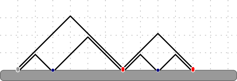
Figure 1: Two directed walks of length 10 of our model that begin and end on the surface. There are two single and two double visits marked. The left-most (start) vertex of the two walks on the wall is not counted as a double visit.

To find the free energy we will instead solve for the generating function

$$G(a,d;z)=\sum_{n=0}^{\infty}Z_{n}(a,d)z^{n}.$$ (2.3)

The radius of convergence of the generating function $z_{c}(a,d)$ is directly related to the free energy via

$$\kappa(a,d)=\log(z_{c}(a,d)^{-1}).$$ (2.4)

3 Functional Equations

To find $G$, we consider walks $\varphi$ in the larger set, where each walk can end at any possible height. Let us first consider $a=d=1$. In this case we construct the expanded generating function

$$F(r,s;z)\equiv F(r,s) =\sum_{\varphi\in\Omega}z^{|\varphi|}r^{\lfloor\varphi\rfloor}s^{\lceil\varphi\rceil/2},$$ (3.1)

where $z$ is conjugate to the length ${|\varphi|}$ of the walk, $r$ is conjugate to the distance ${\lfloor\varphi\rfloor}$ of the bottom walk from the wall and $s$ is conjugate to half the distance ${\lceil\varphi\rceil}$ between the final vertices of the two walks. Since the distance between the endpoints of the walks changes by $0$ or $\pm 2$ with each step, and the endpoints start together, it is always an even number. Further, we let $[r^{j}s^{k}]F(r,s)$ denote the coefficient of $r^{j}s^{k}$ in the generating function $F(r,s)$. We use $[r^{j}]F(r,s)$ to denote the coefficient of $r^{j}$ in $F(r,s)$ which is a function of $s$ and similarly $[s^{k}]F(r,s)$ gives a function of $r$.

Let us now return to general $a$ and $d$. All pairs of walks can then be built using a standard column-by-column construction. Translating this into its action on the generating function gives the following functional equation

$$F(r,s)= 1+z\left(r+\frac{1}{r}+\frac{s}{r}+\frac{r}{s}\right)\cdot F(r,s)$$

$$-z\left(\frac{1}{r}+\frac{s}{r}\right)\cdot[r^{0}]F(r,s)-z\frac{r}{s}\cdot[s^{0}]F(r,s)$$

$$+z(a-1)(1+s)\cdot[r^{1}]F(r,s)+z(d-a)\cdot[r^{1}s^{0}]F(r,s).$$ (3.2)

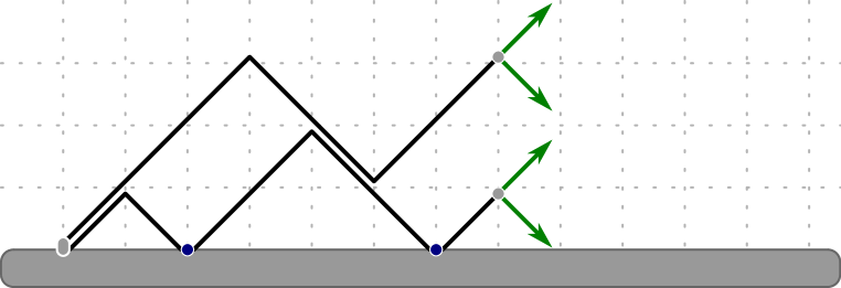
Figure 2: Adding steps to the walks when the walks are away from the wall. There are four possibilities.

We explain each of the terms in this equation.

• The trivial pair of walks of length $0$ gives the initial $1$ in the functional equation.

• Every pair of walks may be extended by appending directed steps to their endpoints in four different ways (see Figure 2).

  Top walk	Bottom walk	Generating Function
  $(1,1)$	$(1,1)$	$r\cdot F(r,s)$
  $(1,1)$	$(1,-1)$	$\frac{s}{r}\cdot F(r,s)$
  $(1,-1)$	$(1,1)$	$\frac{r}{s}\cdot F(r,s)$
  $(1,-1)$	$(1,-1)$	$\frac{1}{r}\cdot F(r,s)$

  

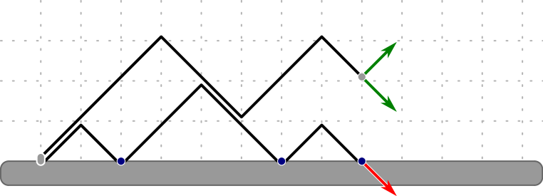
  Figure 3: The first boundary term in the functional equation removes the contribution from the walks that are produced by appending a SE step to the bottom walk when its endpoint is on the wall.

• Appending steps in this way may result in the bottom walk stepping below the wall (Figure 3). Thus, when the bottom walk is at the wall, we cannot append any steps that will decrease the height of the bottom walk. These forbidden configurations are counted by

  $$z\left(\frac{1}{r}+\frac{s}{r}\right)\cdot[r^{0}]F(r,s) =z\left(\frac{1}{r}+\frac{s}{r}\right)\cdot F(0,s).$$ (3.3)

  

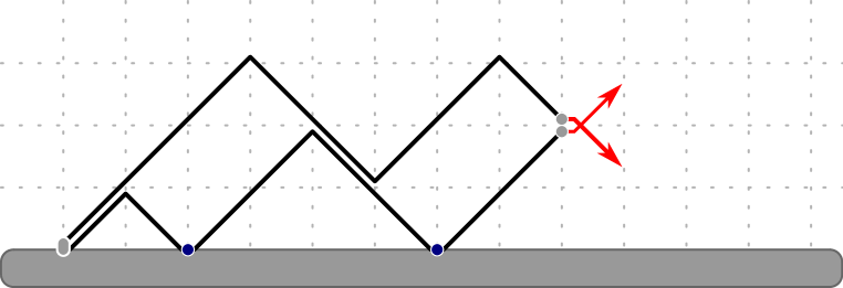
  Figure 4: The second boundary term in the functional equation removes the contribution of walks that cross. Such configurations are produced when one appends steps to walks that end at the same vertex as shown.

• Similarly, at no time can the top walk pass below the bottom walk (Figure 4). Thus, if the two walks are touching, we forbid the distance between them to decrease. These configurations are counted by

  $$z\frac{r}{s}\cdot[s^{0}]F(r,s) =z\frac{r}{s}\cdot F(r,0).$$ (3.4)

• This accounts for the possible pairs of walks without the interaction parameters. We can now incorporate the interaction parameters. In order to do this, we have to add in all walks we want to mark with $a$ and subtract the non-weighted version of those exact same walks from the model (Figure 5 — left). In order for the bottom walk to touch the wall, it must be at height $1$ initially and then step down (with no restriction on the top walk). Hence we get the term

  $$z(a-1)(1+s)\cdot[r^{1}]F(r,s).$$ (3.5)

  

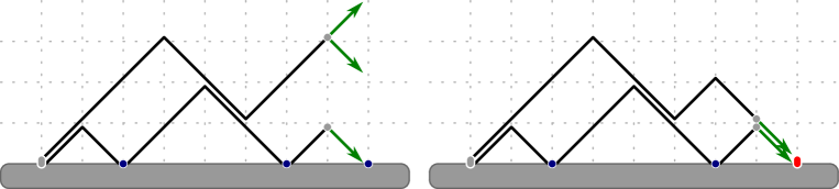
  Figure 5: Configurations that lead to single (left) and double (right) interaction terms.

• A similar method can be used to incorporate $d$ into the model (Figure 5 — right). One step before both walks touch the wall they will both be at height $1$. All such walks have already been accounted for when incorporating $a$ into the model and so must be replaced. This results in

  $$z(d-a)\cdot[r^{1}s^{0}]F(r,s).$$ (3.6)

The functions $[r^{1}]F(r,s)$ and $[r^{1}s^{0}]F(r,s)$ can be simplified in terms of $F(0,0)$ and $F(0,s)$. By extracting the coefficient of $r^{0}s^{0}$ in the functional equation, we obtain

$$F(0,0) =1+zd\cdot[r^{1}s^{0}]F(r,s).$$ (3.7)

At a combinatorial level, this states that a pair of walks that end at the wall is either a trivial configuration or obtained by appending a pair of SE steps to the end of a pair of walks that end at height $1$. Similarly, we can extract the coefficient of $r^{0}$ in the functional equation to obtain

$$F(0,s)=1+za(1+s)\cdot[r^{1}]F(r,s)+z(d-a)\cdot[r^{1}s^{0}]F(r,s).$$ (3.8)

This has a similar combinatorial interpretation to the previous case. These equations can then be combined to simplify the functional equation

$$\left(1-z\left[r+\frac{1}{r}+\frac{s}{r}+\frac{r}{s}\right]\right)\cdot F(r,s)=\\ \frac{1}{d}+\left(1-\frac{1}{a}-\frac{zs}{r}-\frac{z}{r}\right)\cdot F(0,s)-\frac{zr}{s}\cdot F(r,0)+\left(\frac{1}{a}-\frac{1}{d}\right)\cdot F(0,0).$$ (3.9)

We will use the above form of the equation in what follows. The polynomial coefficient on the left hand side is called the kernel $K(r,s;z)\equiv K(r,s)$, and its symmetries play a key role in the solution:

$$K(r,s)=\left[1-z\left(r+\frac{1}{r}+\frac{s}{r}+\frac{r}{s}\right)\right].$$ (3.10)

4 Solution of the functional equations

In what follows we use the obstinate kernel method. The discussion below is self-contained, but we refer the reader to the paper of Bousquet-Mélou and Mishna [34] for a general description of this technique.

4.1 Solution of the functional equations when $a=1$

When $a=1$, the functional equation (3.9) simplifies to

$$K(r,s)\cdot rsdF(r,s)=rs-zsd\left(1+s\right)\cdot F(0,s)-zr^{2}dF(r,0)+rs\left(d-1\right)F(0,0).$$ (4.1)

We use the kernel method which exploits the symmetries of the kernel to remove boundary terms (ie the functions $F(r,0)$ and $F(0,s)$) in the above equation. The kernel is symmetric under the following two transformations:

$$(r,s) \mapsto\left(r,\frac{r^{2}}{s}\right), (r,s) \mapsto\left(\frac{s}{r},s\right).$$ (4.2)

These transformations generate a family of 8 symmetries (sometimes referred to as the ‘group of the walk’ — see [34])

$$(r,s),\left(r,\frac{r^{2}}{s}\right),\left(\frac{s}{r},\frac{s}{r^{2}}\right),\left(\frac{r}{s},\frac{1}{s}\right),\left(\frac{1}{r},\frac{1}{s}\right),\left(\frac{1}{r},\frac{s}{r^{2}}\right),\left(\frac{r}{s},\frac{r^{2}}{s}\right),\text{ and }\left(\frac{s}{r},s\right).$$ (4.3)

We make use of $4$ of these transformations — those which only involve positive powers of $r$. To be precise,

$$K(r,s)\cdot rsdF(r,s) =rs-zsd\left(1+s\right)\cdot F(0,s)-zr^{2}d\cdot F(r,0)+rs\left(d-1\right)\cdot F(0,0);$$ (4.4a)

$$K\left(r,\frac{r^{2}}{s}\right)\cdot\frac{dr^{3}}{s}F\left(r,\frac{r^{2}}{s}\right) =\frac{r^{3}}{s}-\frac{zdr^{2}}{s}\left(1+\frac{r^{2}}{s}\right)\cdot F\left(0,\frac{r^{2}}{s}\right)-zr^{2}d\cdot F(r,0)+\frac{r^{3}}{s}\left(d-1\right)\cdot F(0,0);$$ (4.4b)

$$K\left(\frac{r}{s},\frac{r^{2}}{s}\right)\cdot\frac{dr^{3}}{s^{2}}F\left(\frac{r}{s},\frac{r^{2}}{s}\right) =\frac{r^{3}}{s^{2}}-\frac{zdr^{2}}{s}\left(1+\frac{r^{2}}{s}\right)\cdot F\left(0,\frac{r^{2}}{s}\right)-\frac{zr^{2}d}{s^{2}}\cdot F(\frac{r}{s},0)+\frac{r^{3}}{s^{2}}\left(d-1\right)\cdot F(0,0);$$ (4.4c)

$$K\left(\frac{r}{s},\frac{1}{s}\right)\cdot\frac{dr}{s^{2}}F\left(\frac{r}{s},\frac{1}{s}\right) =\frac{r}{s^{2}}-\frac{zd}{s}\left(1+\frac{1}{s}\right)\cdot F\left(0,\frac{1}{s}\right)-\frac{zdr^{2}}{s^{2}}\cdot F\left(\frac{r}{s},0\right)+\frac{r(d-1)}{s^{2}}\cdot F(0,0).$$ (4.4d)

All of these transformations were chosen so that the kernel remains unchanged, and so that the substitution only involves positive powers of $r$. We can then eliminate the boundary terms by taking an alternating sum of the above equations:

$$\text{Eqn(\ref{eqn symm1})}-\text{Eqn(\ref{eqn symm2})}+\text{Eqn(\ref{eqn symm3})}-\text{Eqn(\ref{eqn symm4})}.$$

(In the case where $a\neq 1$, a similar method holds, except that then we must multiply some of the equations by non-trivial coefficients to eliminate boundary terms.) After simplification we obtain

$$K(r,s)\cdot\left(\text{linear combination of }F\right)=\\ \frac{r(s-1)(s^{2}+s+1-r^{2})}{s^{2}}\left(1+(d-1)F(0,0)\right)\\ -zd(1+s)sF(0,s)+\frac{zd(1+s)}{s^{2}}F\left(0,\frac{1}{s}\right).$$ (4.5)

We can now remove the left-hand side of the equation by choosing a value of $r$ that sets the kernel to zero — provided all the $F$’s on the left-hand side remain convergent. The kernel has two roots and we choose the one which gives a positive term power series expansion in $z$ with Laurent polynomial coefficients in $s$:

$$\hat{r}(s;z)\equiv\hat{r} =\frac{s\left(1-\sqrt{1-4\frac{(1+s)^{2}z^{2}}{s}}\right)}{2(1+s)z}=\sum_{n\geq 0}C_{n}\frac{(1+s)^{2n+1}z^{2n+1}}{s^{n}},$$ (4.6)

where $C_{n}=\frac{1}{n+1}\binom{2n}{n}$ is a Catalan number. This is chosen so that $K(\hat{r},s)=0$, and so that all the various substitutions are convergent. More precisely, since $\hat{r}=O(z)$, the functions $F(\hat{r},s),F(\hat{r},\hat{r}^{2}/s),F(\hat{r}/s,\hat{r^{2}}/s)$ and $F(\hat{r}/s,1/s)$ are all formally convergent power series in $z$ with Laurent polynomial coefficients in $s$.

We are not able to use the other root of the kernel (with respect to $r$) since it is $O(z^{-1})$. If we were to substitute this into the functional equation, then $F(r,s),F(r,r^{2}/s),F(r/s,r^{2}/s)$ and $F(r/s,1/s)$ would not converge within the ring of formal power series. This follows since the coefficient of $z^{n}$ in $F(r,s)$ has degree $n$ in $r$ and so substituting $r\mapsto O(z^{-1})$ will map terms in this polynomial to all powers of $z$ including the constant term.

When we make the substitution $r\mapsto\hat{r}$ we can rewrite the coefficients of the right-hand side so as to not explicitly involve $z$ — since now $z=\left(\hat{r}+1/\hat{r}+\hat{r}/s+s/\hat{r}\right)^{-1}$.

$$0 =\frac{\hat{r}(s-1)(s^{2}+s+1-\hat{r}^{2})}{s^{2}}\left(1+(d-1)F(0,0)\right)-\frac{d\hat{r}s^{2}}{s+\hat{r}^{2}}\,F(0,s)+\frac{d\hat{r}}{(s+\hat{r}^{2})s}\,F\left(0,\frac{1}{s}\right).$$ (4.7)

Because we are primarily interested in $F(0,0)$ — the generating function of pairs of walks that start and end on the wall — it is convenient to rewrite the equation so that there are no powers of $s$ or $\hat{r}$ in the denominator of the coefficients and so that the coefficients of $F(0,s)$ and $F(0,1/s)$ are independent of $\hat{r}$.

$$0 =ds^{4}F(0,s)-dsF\left(0,\frac{1}{s}\right)-(s-1)(s^{2}+s+1-\hat{r}^{2})(s+\hat{r}^{2})\left(1+(d-1)F(0,0)\right).$$ (4.8)

Consider the coefficient of $s^{1}$ in the above equation, or rather by dividing the equation by $s$ consider the constant term, that is the coefficient of $s^{0}$ in the equation. This leads us to calculate $F(0,0)$ effectively as a constant term in the variable $s$. For ease of calculation and display we will continue with calculating the coefficient of $s^{1}$ in equation (4.8).

Since $F(0,s)$ is a power series in $z$ with polynomial coefficients in $s$, the term $ds^{4}F(0,s)$ does not contain any coefficients of $s^{1}$. Similarly, $F\left(0,\frac{1}{s}\right)$ is a power series in $z$ with polynomial coefficients in $s^{-1}$, so the term $dsF\left(0,\frac{1}{s}\right)$ contributes only $dF(0,0)$. For the remaining term, we consider the coefficient $[s^{1}](s-1)(s^{2}+s+1-\hat{r}^{2})(s+\hat{r}^{2})$. Expanding the expression and then collecting the exponents of $\hat{r}$ gives:

$$(s-1)\hat{r}^{4}+(1-s+s^{2}-s^{3})\hat{r}^{2}+s(1-s)(s^{2}+s+1).$$ (4.9)

We need to consider the expansion of $\hat{r}^{2}$ and $\hat{r}^{4}$. Lagrange inversion [35] gives:

$$\hat{r}(s;z) =\sum_{n=0}^{\infty}\frac{C_{n}(1+s)^{2n+1}}{s^{n}}z^{2n+1},$$ (4.10a)

$$\hat{r}(s;z)^{2} =\sum_{n=0}^{\infty}\frac{C_{n+1}(1+s)^{2n+2}}{s^{n}}z^{2n+2},$$ (4.10b)

$$\hat{r}(s;z)^{4} =\sum_{n=0}^{\infty}\frac{4}{2n+4}\binom{2n+4}{n}\frac{(1+s)^{2n+4}}{s^{n}}z^{2n+4},$$ (4.10c)

and, more generally,

$$\hat{r}(s;z)^{k} =\sum_{n=0}^{\infty}\frac{k}{2n+k}\binom{2n+k}{n}\frac{(1+s)^{2n+k}}{s^{n}}z^{2n+k}.$$ (4.10d)

Computing the coefficient of a particular power of $s$ in $\hat{r}^{2}$ or $\hat{r}^{4}$ reduces to finding the coefficient of powers of $s$ in $(1+s)^{n}s^{-k}$ which are just binomial coefficients:

$$[s^{1}](s-1)\hat{r}^{4} =\sum_{n=0}^{\infty}-\frac{6(n-1)n}{(n+2)^{2}}C_{n}^{2}z^{2n+2};$$ (4.11a)

$$[s^{1}](1-s+s^{2}-s^{3})\hat{r}^{2} =\sum_{n=0}^{\infty}\frac{6(n^{2}+1)}{(n+2)(n+3)}C_{n}^{2}z^{2n+2};$$ (4.11b)

$$[s^{1}]s(1-s)(s^{2}+s+1) =1;$$ (4.11c)

$$[s^{1}](s-1)(s^{2}+s+1-\hat{r}^{2})(s+\hat{r}^{2}) =1+\sum_{n=0}^{\infty}\frac{12(2n+1)}{(n+2)^{2}(n+3)}C_{n}^{2}z^{2n+2}.$$ (4.11d)

Hence extracting the coefficient of $s^{1}$ in equation (4.8) gives

$$0 =-\left(1+\sum_{n=0}^{\infty}\frac{12(2n+1)}{(n+2)^{2}(n+3)}C_{n}^{2}z^{2n+2}\right)\cdot\left(1+(d-1)F(0,0)\right)-d\cdot F(0,0).$$ (4.12)

Solving the above when $d=1$ gives

$$G(1,1;z) =1+\sum_{n=0}^{\infty}\frac{12(2n+1)}{(n+2)^{2}(n+3)}C_{n}^{2}z^{2n+2},$$ (4.13)

and hence for general $d$ we have

$$F(0,0)=G(1,d;z) =\frac{G(1,1;z)}{d+(1-d)G(1,1;z)}.$$ (4.14)

In Section 5 we will see that the algebraic structure of this solution that gives $G(1,d;z)$ in terms of $G(1,1;z)$ arises naturally from a combinatorial construction. Moreover, this structure extends to the $a\neq 1$ case.

4.2 Solution of the functional equation when $a\neq 1$

The general $a,d$ case can be solved by the method applied above, however, it is sufficient to study the case $d=a$ which can be resolved more cleanly. As mentioned above the algebraic structure that allows $G(1,d;z)$ to be expressed in terms of $G(1,1;z)$ extends to give $G(a,d;z)$ in terms of $G(a,a;z)$. We shall see that explicitly in Section 5. When $d=a$ the functional equation (3.9) simplifies to

$$K(r,s)\cdot F(r,s)a^{2}rs =(ar-r-za-zas)as\cdot F(0,s)-zr^{2}a^{2}\cdot F(r,0)+ars.$$ (4.15)

The symmetries we used above can be reused to remove boundary terms. As above we take an alternating sum of transformed equations, but now we must multiply some of the equations by a non-trivial factor chosen to eliminate boundary terms. The left-hand side becomes

$$LHS =a^{2}rK(r,s)\left(sF(r,s)-\frac{r^{2}}{s}F\left(r,\frac{r^{2}}{s}\right)+\frac{Lr^{2}}{s^{2}}F\left(\frac{r}{s},\frac{r^{2}}{s}\right)-\frac{L}{s^{2}}F\left(\frac{r}{s},\frac{1}{s}\right)\right),$$ (4.16)

where

$$L =\frac{zas-ars+rs+zar^{2}}{zas-ar+r+zar^{2}}.$$ (4.17)

The right-hand side simplifies to

$$RHS=as^{2}(1+s-a)F(0,s)+a(1+s-as)F\left(0,1/s\right)\\ -\frac{(r^{2}+s)a(s-1)(ar^{2}+as-2s-s^{2}-1)}{ar^{2}-r^{2}-s}.$$ (4.18)

Again, we have attempted to massage the functional equation into a form in which the coefficients of $F(0,s)$ and $F(0,1/s)$ are independent of $r$. Unfortunately, we cannot completely clear the denominator of the above functional equation, and we found it simplest to work with the above expression.

Following the method used in the $a=1$ case, we can eliminate the left-hand side further by choosing a value of $r$ that sets the kernel to $0$. We choose the root which gives a positive term power series expansion in $z$ with Laurent polynomial coefficients in $s$. Recall that $\hat{r}$ is given by

$$\hat{r}(s;z)\equiv\hat{r} =\sum_{n\geq 0}C_{n}\frac{(1+s)^{2n+1}z^{2n+1}}{s^{n}}.$$ (4.19)

Substituting $r\mapsto\hat{r}$ eliminates the left-hand side of the functional equation and we again consider the coefficient of $s^{1}$ in the resulting right-hand side. Again, this can be converted into a constant term expression for our generating function. The term $as^{2}(1+s-a)F(0,s)$ does not contribute to $s^{1}$. The term $a(1+s-as)F\left(0,1/s\right)$ contributes $a(1-a)F\left(0,0\right)$. For the remaining term, we consider the expansion of the expression as a series in $a$. The coefficient of $a^{1}$ is

$$[a^{1}]\frac{a(\hat{r}^{2}+s)(s-1)(a\hat{r}^{2}+as-2s-s^{2}-1)}{a\hat{r}^{2}-\hat{r}^{2}-s} =(1-s)(1+s)^{2},$$ (4.20)

and hence

$$[a^{1}s^{1}]\frac{a(\hat{r}^{2}+s)(s-1)(a\hat{r}^{2}+as-2s-s^{2}-1)}{a\hat{r}^{2}-\hat{r}^{2}-s} =-1.$$ (4.21)

Higher powers of $a$ are (for $k\geq 1$)

$$[a^{k+1}]\frac{a(\hat{r}^{2}+s)(s-1)(a\hat{r}^{2}+as-2s-s^{2}-1)}{a\hat{r}^{2}-\hat{r}^{2}-s}\\ \begin{split}=&\frac{(s-1)(\hat{r}-1)(\hat{r}+1)(\hat{r}-s)(\hat{r}+s)}{\hat{r}^{2}}\cdot\left(\frac{\hat{r}^{2}}{s+\hat{r}^{2}}\right)^{k}\\ =&\left(\frac{(s-1)s^{2}}{(s+1)^{2}z^{2}}-(s+1)^{2}(s-1)\right)\cdot\left(\frac{\hat{r}^{2}}{s+\hat{r}^{2}}\right)^{k}\\ =&\left(\frac{(s-1)s^{2}}{(s+1)^{2}z^{2}}\right)\cdot\left(\frac{\hat{r}^{2}}{s+\hat{r}^{2}}\right)^{k}-\left((s+1)^{2}(s-1)\right)\cdot\left(\frac{\hat{r}^{2}}{s+\hat{r}^{2}}\right)^{k}.\end{split}$$ (4.22)

To extract the coefficient of $s^{1}$, we need to consider the expansion of $\left(\frac{\hat{r}^{2}}{s+\hat{r}^{2}}\right)^{k}$ in $z$. This exponential term simplifies, and we can use equation (4.10d) to obtain

$$\left(\frac{\hat{r}^{2}}{s+\hat{r}^{2}}\right)^{k}=z^{k}\left(\frac{1+s}{s}\right)^{k}\hat{r}^{k} =\sum_{p\geq 0}\frac{k}{2p+k}\binom{2p+k}{p}\frac{(s+1)^{2p+2k}}{s^{p+k}}z^{2p+2k}.$$ (4.23)

We will expand the two terms in (4.22) individually. For the first term, we get

$$[s^{1}]\frac{(s-1)s^{2}}{(s+1)^{2}z^{2}}\cdot\left(\frac{\hat{r}^{2}}{s+\hat{r}^{2}}\right)^{k}\\ =\sum_{p\geq 0}\frac{k}{k+2p}\binom{k+2p}{p}\left(\binom{2k-2+2p}{k+p-1}-\binom{2k-2+2p}{k+p-2}\right)z^{2k-2+2p}.$$ (4.24)

We can extract the coefficient of $z^{2n}$ from the above equation by making the substitution $n=k-1+p$. We obtain

$$[z^{2n}s^{1}]\frac{(s-1)s^{2}}{(s+1)^{2}z^{2}}\cdot\left(\frac{\hat{r}^{2}}{s+\hat{r}^{2}}\right)^{k} =\frac{k}{2n-k+2}\binom{2n-k+2}{n+1}\left[\binom{2n}{n}-\binom{2n}{n-1}\right].$$ (4.25)

Therefore

$$[s^{1}]\frac{(s-1)s^{2}}{(s+1)^{2}z^{2}}\cdot\left(\frac{\hat{r}^{2}}{s+\hat{r}^{2}}\right)^{k} =\sum_{n\geq k-1}\frac{k}{2n-k+2}\binom{2n-k+2}{n+1}\left[\binom{2n}{n}-\binom{2n}{n-1}\right]z^{2n}.$$ (4.26)

Following a similar argument for the second term in equation (4.22), we have

$$[s^{1}](s+1)^{2}(s-1)\cdot\left(\frac{\hat{r}^{2}}{s+\hat{r}^{2}}\right)^{k}\\ =\sum_{p\geq 0}\frac{k}{k+2p}\binom{k+2p}{p}\left(\binom{2k+2p+2}{k+p}-\binom{2k+2p+2}{k+p-1}\right)z^{2k+2p}.$$ (4.27)

Making the substitution $n=k+p$, we get

$$[z^{2n}s^{1}](s+1)^{2}(s-1)\cdot\left(\frac{\hat{r}^{2}}{s+\hat{r}^{2}}\right)^{k} =\frac{k}{2n-k}\binom{2n-k}{n}\left[\binom{2n+2}{n+1}-\binom{2n+2}{n}\right].$$ (4.28)

We can then substitute the summation over $p$ with a summation over $n$.

$$[s^{1}](s+1)^{2}(s-1)\cdot\left(\frac{\hat{r}^{2}}{s+\hat{r}^{2}}\right)^{k} =\sum_{n\geq k}\frac{k}{2n-k}\binom{2n-k}{n}\left[\binom{2n+2}{n+1}-\binom{2n+2}{n}\right]z^{2n}.$$ (4.29)

When $n=k-1$ in the above equation, the summand reduces to $0$ when $k>2$. So it is possible to adjust the range of the summation by adjusting for the $k=1,2$ cases separately. In those cases, the combined correction terms are $a^{2}$ and $-4a^{3}z^{2}$ respectively. Thus, we can rewrite

$$[s^{1}](s+1)^{2}(s-1)\cdot\left(\frac{\hat{r}^{2}}{s+\hat{r}^{2}}\right)^{k}\\ =\sum_{n\geq k-1}\frac{k}{2n-k}\binom{2n-k}{n}\left[\binom{2n+2}{n+1}-\binom{2n+2}{n}\right]z^{2n},$$ (4.30)

with known correction terms for $k=1,2$. Combining these summands, we get that for $n\geq k-1$:

$$\frac{k}{2n-k+2}\binom{2n-k+2}{n+1}\left[\binom{2n}{n}-\binom{2n}{n-1}\right]\\ -\frac{k}{2n-k}\binom{2n-k}{n}\left[\binom{2n+2}{n+1}-\binom{2n+2}{n}\right]\\ =\frac{k(k+1)(2+4n-kn-2k)}{(k-1-n)(n+1)^{2}(k-2n)(n+2)}\binom{2n-k}{n}\binom{2n}{n}.$$ (4.31)

Thus taking the coefficient of $s^{1}$ when $r=\hat{r}$ in equation (4.18) and accounting for the correction terms, we get

$$0=a(a-1)F(0,0)-a+a^{2}-4z^{2}a^{3}\\ -\sum_{k\geq 1}a^{k+1}\sum_{n\geq k-1}\frac{k(k+1)(2+4n-kn-2k)}{(k-1-n)(n+1)^{2}(-2n+k)(n+2)}\binom{2n-k}{n}\binom{2n}{n}z^{2n}.$$ (4.32)

We exchange the order of summation to give

$$0=a(a-1)F(0,0)-a+a^{2}-4z^{2}a^{3}\\ -\sum_{n\geq 0}z^{2n}\sum_{k=1}^{n+1}\frac{k(k+1)(2+4n-kn-2k)}{(k-1-n)(n+1)^{2}(-2n+k)(n+2)}\binom{2n-k}{n}\binom{2n}{n}a^{k+1}.$$ (4.33)

The extraction of the coefficient $[a^{k}z^{2n}]F(0,0)$ requires rearranging the $a(a-1)$ coefficient in front of $F(0,0)$. We express the above equation as:

$$0=a(a-1)F(0,0)-\sum_{n\geq 0}z^{2n}\sum_{k^{\prime}=1}^{n+1}Q_{n,k^{\prime}}a^{k^{\prime}+1}$$ (4.34)

for some integers $Q_{n,k^{\prime}}$. This can be rearranged to give:

$$F(0,0) =-\left(\sum_{n\geq 0}z^{2n}\sum_{k^{\prime}=1}^{n+1}Q_{n,k^{\prime}}a^{k^{\prime}}\right)\cdot\frac{1}{1-a}$$ (4.35)

$$=-\left(\sum_{n\geq 0}z^{2n}\sum_{k^{\prime}=1}^{n+1}Q_{n,k^{\prime}}a^{k^{\prime}}\right)\cdot\left(\sum_{k^{\prime\prime}\geq 0}a^{k^{\prime\prime}}\right).$$ (4.36)

The coefficient of $a^{k}$ from the above is summation of all contributions from $k^{\prime}$ and $k^{\prime\prime}$ such that $k^{\prime}+k^{\prime\prime}=k$. Thus:

$$F(0,0)=\sum_{n\geq 0}z^{2n}\sum_{k=1}^{n+1}a^{k}\sum_{k^{\prime}=1}^{k}Q_{n,k^{\prime}}.$$ (4.37)

In other words, extracting the coefficient $[a^{k}z^{2n}]F(0,0)$ requires a summation of a finite number of the $Q_{n,k^{\prime}}$ terms which is obtained from (4.33).

$$[a^{k}z^{2n}]F(0,0) =\sum_{k^{\prime}=0}^{k}\frac{k^{\prime}(k^{\prime}+1)(2+4n-k^{\prime}n-2k^{\prime})}{(k^{\prime}-1-n)(n+1)^{2}(-2n+k^{\prime})(n+2)}\binom{2n-k^{\prime}}{n}\binom{2n}{n}$$ (4.38)

$$=\frac{k(k+1)(k+2)}{(2n-k)(n+1)^{2}(n+2)}\binom{2n-k}{n}\binom{2n}{n}.$$ (4.39)

We finally obtain

$$F(0,0)=G(a,a) =\sum_{n\geq 0}z^{2n}\sum_{k=0}^{n}a^{k}\frac{k(k+1)(k+2)}{(n+1)^{2}(n+2)(2n-k)}\binom{2n}{n}\binom{2n-k}{n}.$$ (4.40)

This agrees with results due to Brak et al.  [36, 37] for a closely related model obtained using very different method — we discuss this more fully in the section 5.

5 Alternate solution

An alternate technique for finding the generating function relies on factoring the pairs of walks at each double-visit. First, let us define

$$G(a,d)\equiv G(a,d;z) =F(0,0;a,d;z).$$ (5.1)

We will frequently hide the $z$ dependence for convenience. Breaking up our configurations into pieces between double visits gives

$$G(a,d;z) =\frac{1}{1-dP(a;z)},$$ (5.2)

where $P(a;z)$ is the generating function of so-called primitive factors. This is quite analogous to the classical factorisation of a single Dyck path. These primitive factors are pairs of friendly Dyck-paths which contain no double-visits to the surface other than their first and last vertices. Rearranging this expression gives

$$P(a;z) =\frac{G(a,d;z)-1}{dG(a,d;z)}=\frac{G(a,a;z)-1}{aG(a,a;z)}.$$ (5.3)

This last expression allows us to calculate $P(a;z)$ from a known expression for $G(a,a;z)$ — such as that given in the previous section. Alternatively, one could use results from previous work by Brak et al.  [36, 37]. In those works, the authors considered a vesicle model which corresponds exactly to the case $d=a$ — their vicious walk model can be transformed into the friendly walk model considered here, by moving the upper vesicle boundary down by 2 units.

Brak et al. use the Lindström-Gessel-Viennot lemma [31, 32] to express the partition function of the pair of walks in terms of the partition function of a single walk. Namely,

$$[z^{n}]G(a,a) =\frac{S_{2n}(1)S_{2n+4}(a)-S_{2n+2}(1)S_{2n+2}(a)}{a^{2}},$$ (5.4)

where $S_{2n}(a)$ is the partition function of a single Dyck path of length $2n$ above a wall, and $a$ is conjugate to the number of visits, ie

$$S_{2n}(a) =[z^{2n}]\,2\left(2-a+a\sqrt{1-4z^{2}}\right)^{-1}$$ (5.5)

$$=\sum_{k=0}^{n}\frac{2k+1}{n+k+1}\binom{2n}{n-k}(a-1)^{k}=\sum_{k=1}^{n}\frac{k}{2n-k}\binom{2n-k}{n}a^{k},$$ (5.6)

where this last formula is taken from [36]. When $a=1$ we recover the well-known Catalan number result, and a well-known central binomial result when $a=2$:

$$S_{2n}(1) =C_{n}=\frac{1}{n+1}\binom{2n}{n}, S_{2n}(2) =\binom{2n}{n}.$$ (5.7)

In light of these simple expressions one can write $G(a,a;z)$ as double sum of products of binomials. Using equation (5.3) we write $G(a,d;z)$ in terms of $G(a,a;z)$

$$G(a,d) =\frac{aG(a,a)}{d+(a-d)G(a,a)},$$ (5.8)

where

$$G(a,a) =a^{-2}\sum_{n=0}^{\infty}\left[C_{n}S_{2n+4}(a)-C_{n+1}S_{2n+2}(a)\right]z^{2n},$$ (5.9)

which simplifies to the expression in equation (4.40) found in the previous section.

5.1 Solutions at $a=0,1$ and $2$

Since the partition function $S_{2n}(a)$ takes simple values at $a=0,1,2$, we have

$$G(1,1;z) =\sum_{n=0}^{\infty}\left[C_{n}C_{n+2}-C_{n+1}^{2}\right]z^{2n},$$

$$=\sum_{n=0}^{\infty}\frac{12(2n+1)}{(n+1)^{2}(n+2)^{2}(n+3)}\binom{2n}{n}^{2}z^{2n},$$ (5.10)

$$G(2,2;z) =\sum_{n=0}^{\infty}C_{n}C_{n+1}z^{2n},$$ (5.11)

and

$$\lim_{a\to 0}\frac{G(a,a;z)-1}{a} =\sum_{n=1}^{\infty}\frac{12(2n-1)}{n^{2}(n+1)^{2}(n+2)}\binom{2n-2}{n-1}^{2}z^{2n}=z^{2}G(1,1;z).$$ (5.12)

We can use these together with equation (5.8) to derive expressions for $G(1,d)$ (that agrees with (4.13) and (4.14)) and $G(2,d)$ by simple substitutions. That is,

$$G(1,d) =\frac{\sum_{n=0}^{\infty}\frac{12(2n+1)}{(n+1)^{2}(n+2)^{2}(n+3)}\binom{2n}{n}^{2}z^{2n}}{d+(1-d)\sum_{n=0}^{\infty}\frac{12(2n+1)}{(n+1)^{2}(n+2)^{2}(n+3)}\binom{2n}{n}^{2}z^{2n}}$$ (5.13)

and

$$G(2,d) =\frac{2\sum_{n=0}^{\infty}C_{n}C_{n+1}z^{2n}}{d+(2-d)\sum_{n=0}^{\infty}C_{n}C_{n+1}z^{2n}}.$$ (5.14)

A little further work also gives

$$G(0,d) =\frac{1}{1-dz^{2}G(1,1)}=\frac{1}{1-dz^{2}\sum_{n=0}^{\infty}\frac{12(2n+1)}{(n+1)^{2}(n+2)^{2}(n+3)}\binom{2n}{n}^{2}z^{2n}}.$$ (5.15)

This last expression can be derived combinatorially by noting that in the limit $a\to 0$ single visits are forbidden. In this limit, the primitive pieces are in bijection with all walks counted by $G(1,1)$; any primitive piece can be transformed into a pair of walks counted by $G(1,1)$ by moving them 1 lattice unit up and gluing edges at the start and end.

6 Analysis of phase structure and transitions

6.1 Phases

We now turn to the phase diagram of the model which is dictated by the radius of convergence of $G(a,d;z)$ as a power series in $z$. Denote the radius of convergence by $z_{c}(a,d)$. Equation (5.2) shows that the singularities of $G(a,d;z)$ are those of $P(a;z)$ and the simple pole at $1-dP(a;z)=0$. Denote this latter singularity by $z_{d}(a,d)$. Equation (5.3) shows that the singularities of $P(a;z)$ are related to those of $G(a,a;z)$ which are known from [36, 37].

In particular, the radius of convergence of $G(a,a;z)$ is

$$\rho(a)=\text{r.o.c }G(a,a;z) =\begin{cases}\frac{1}{4}=z_{b}&a\leq 2,\\ \frac{\sqrt{a-1}}{2a}=z_{a}(a)&a>2.\end{cases}$$ (6.1)

For $a<2$, the thermodynamic phase is related to $z_{b}$ and is the desorbed phase in which the walks drift away from the wall and the mean number of visits is $O(1)$. When $a>2$, $z_{a}(a)$ dominates and the lower walk adsorbs onto the wall and the number of visits is $O(n)$. At $a=2$, there is a second-order phase transition and a jump discontinuity in the specific heat (the second derivative of the free energy). In both of these phases, the upper walk drifts away from the wall, and the number of doubly-visited vertices is $O(1)$.

In the full $a$-$d$ model there are 3 phases, two of which are described in the previous paragraph. In the third phase, associated with the simple pole at $z_{d}(a,d)$, we shall see that the number of doubly-visited vertices is $O(n)$. In what follows, we name these three phases associated with $z_{b},z_{a}$ and $z_{d}$, desorbed, $a$-rich and $d$-rich respectively.

6.2 Desorbed to $a$-rich transition

In [36], it was shown that the asymptotic behaviour of the singular part of $G(a,a;z)$ near its radius of convergence is given by

$$G(a,a;z) \sim\begin{cases}A_{-}(1-4z)^{4}\log(1-4z)&a<2,\\ A_{0}(1-4z)^{2}\log(1-4z)&a=2,\\ A_{+}\left(1-z/z_{a}(a)\right)^{1/2}&a>2,\end{cases}$$ (6.2)

where $z_{a}(a)=\frac{\sqrt{a-1}}{2a}$. It is important to notice that for all $a$, the singularities are convergent and therefore $G(a,a;z)$ is convergent on its radius of convergence $\rho(a)$.

If we fix $d$ at some small value, and then increase $z$ from 0 towards $\rho(a)$, then $P(a;z)$ increases from $0$ to $P(a;\rho(a))$. Since $d$ is small, and $P(a;\rho(a))$ is finite, $1-dP(a;\rho(a)>0$ and so the only singularities of $G(a,d;z)$ will be those of $P(a;z)$ and so those of $G(a,a;z)$.

Thus for small values of $d$ there is a phase transition on moving $a$ through $2$ which describes the transition from the desorbed phase to an $a$-rich phase as occurs in [36]. This adsorption transition has been well-studied previously and is unusual in that it has a jump discontinuity in the second derivative of the free-energy rather than a divergence.

6.3 Desorbed to $d$-rich transition

Let us restrict our attention to $a<2$ and consider the effect of increasing $d$. The argument in the previous subsection breaks down as soon as $1-dP(a;\rho(a))=0$. Call this value $d_{c}(a)=P(a;\rho(a))^{-1}$.

Fix $a<2$ and $d>d_{c}$ and consider increasing $z$ from $0$ towards $\rho(a)=1/4$. The function $P(a;z)$ is an increasing function of $z$ (since it is a positive term power series) and so it increases towards $P(a;\rho(a))$. Since $d>d_{c}$, $P(a;z)$ will reach the value $d^{-1}$ before it reaches $P(a,\rho(a))$ and the simple pole will occur when $z=z_{d}$, where $z_{d}$ is the solution of

$$P(a;z_{d}(a,d)) =d^{-1}$$ (6.3)

and $z_{d}<z_{b}=1/4$ in this region.

Hence, for $a<2$, there is a phase transition where $z_{d}$ and $z_{b}$ coincide at

$$d_{c}(a) =P(a;1/4)^{-1}=\frac{aG(a,a;1/4)}{G(a,a;1/4)-1}.$$ (6.4)

In order to determine the density of the singly- and doubly-visited vertices in the $d>d_{c}$ phase consider the partial derivatives of $z_{d}(a,d)$ with respect to $a$ and $d$. Since $z_{d}(a,d)$ is defined by $dP(a;z_{d}(a,d))=1$, the derivatives of $z_{d}(a,d)$ with respect to $a$ and $d$ are non-zero and so there are positive densities of both singly- and doubly-visited vertices.

Now let us turn to the order of this transition; this can be determined by examining the behaviour of $P(a;z)$ close to $z=1/4$ which is determined by the behaviour of $G(a,a;z)$ — see equation (5.3). Close to $z=1/4$ we can write

$$G(a,a;z) =G_{analytic}(a;z)+G_{singular}(a;z),$$ (6.5)

where the behaviour of $G_{singular}$ is given by equation (6.2). Consider an expansion of $G_{analytic}$ about $z=1/4$

$$G_{analytic}(a;z) \approx G(a,a;1/4)+c_{1}(1-4z)+\cdots$$ (6.6)

for some non-zero constant $c_{1}$. The linear correction dominates the dominant singular term in $G_{singular}$. Expanding equation (6.3) about $z=1/4$ gives

$$\frac{1}{d_{c}}-\frac{1}{d} =P(a;1/4)-P(a;z_{d}),$$

$$\frac{d-d_{c}}{d_{c}^{2}} \approx p_{1}(1-4z_{d})$$ (6.7)

for some non-zero constant $p_{1}$. Hence there is a linear relationship between the location of the $d$-rich singularity, $z_{d}$, and the distance from the phase boundary. Since the free-energy of the system is $-\log z_{d}$, this also implies the free-energy in the $d$-rich phase changes linearly with $d$. On the other hand in the desorbed phase where $z_{b}$ dominates, the free-energy is a constant. From this we see that there is a jump discontinuity in the first derivative of the free-energy and hence this is a first-order transition. Note that the above argument will also work mutatis mutandis at $a=2$.

We can observe at finite length a characteristic bimodal probability distribution in the number of doubly-visited vertices — see Figure 6.

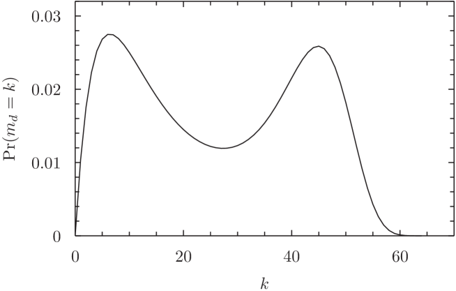
Figure 6: A plot of the probability that a conformation of length 128 has $k$ doubly-visited sites at $a=1,d=10.3$. This value of $d$ corresponds to the approximate location of the peak in the specific heat at this length.

6.4 $a$-rich to $d$-rich transition

The analysis of the previous section can be adapted to the case $a>2$ with some important differences. The transition is driven by the singularities $z_{a}(a)=\frac{\sqrt{a-1}}{2a}$ associated with single-visit adsorption, and the singularity $z_{d}(a,d)$ associated with double-visit adsorption. Again, $z_{d}(a,d)$ is the solution of equation (6.3). These two singularities coincide when $d=d_{c}(a)$ given by

$$d_{c}(a) =P\left(a;\frac{\sqrt{a-1}}{2a}\right)^{-1}=\frac{aG\left(a,a;\frac{\sqrt{a-1}}{2a}\right)}{G\left(a,a;\frac{\sqrt{a-1}}{2a}\right)-1}.$$ (6.8)

Turning to the order of this transition, we again decompose $G(a,a;z)$ into its analytic and singular parts. Observe that close to $z_{a}(a)$, $G_{singular}$, given by equation (6.2), dominates the linear part of $G_{analytic}$. Hence we deduce that

$$d_{c}(a)-d \approx p_{2}\left(\frac{\sqrt{a-1}}{2a}-z_{d}(a,d)\right)^{1/2},$$ (6.9)

$$z_{d}(a,d) \approx\frac{\sqrt{a-1}}{2a}+p_{3}\left(d-d_{c}(a)\right)^{2}$$ (6.10)

for some nonzero constants $p_{2},p_{3}$. Therefore the free-energy has a jump discontinuity in its second derivative on varying $d$ across the transition, and this is a second-order phase transition. This is very similar to the desorbed to $a$-rich transition.

6.5 Phase diagram

We have established that there are 3 thermodynamic phases; desorbed, $a$-rich and $d$-rich. We remind the reader that $m_{a}(\varphi)$ and $m_{d}(\varphi)$ denote the number of single and double visits of $\varphi$.

If we define

$${\cal{A}}(a,d) =\lim_{n\rightarrow\infty}\frac{\langle m_{a}\rangle}{n} {\cal{D}}(a,d) =\lim_{n\rightarrow\infty}\frac{\langle m_{d}\rangle}{n},$$ and (6.11)

then in the desorbed phase we have

$${\cal{A}} ={\cal{D}}=0,$$ (6.12)

while in the $a$-rich phase we have

$${\cal{A}} >0 {\cal{D}}=0,$$ and (6.13)

and in the $d$-rich phase has both

$${\cal{A}} >0 {\cal{D}}>0.$$ and (6.14)

In Figures 7 and  8 we plot $\frac{\langle m_{a}\rangle}{256}$ and $\frac{\langle m_{d}\rangle}{256}$ respectively.

Figure 7: A plot of the density of $a$ visits calculated at length $n=256$. This highlights the region where it tends to a non-zero constant and corresponds well to the regions where $z_{a}$ and $z_{d}$ dominate. Note that for fixed $a$ and increasing, large $d$ we expect that the density of $a$ visits decreases though remains positive.

Figure 8: A plot of the density of $d$ visits calculated at length $n=256$. This highlights the region where it is tends to a non-zero constant and corresponds well to the region where we have shown that $z_{d}$ is the dominant singularity.

The phase boundary between the desorbed and $a$-rich phases occurs at

$$a =2 \mbox{for $d<d_{c}(2)$}.$$ (6.15)

Note that this phase boundary is, unsurprisingly, independent of $d$. We can compute $d_{c}(2)$ exactly using the results of Section 5.1:

$$G(2,2;1/4) =\sum_{n\geq 0}C_{n}C_{n+1}16^{-n}=8-\frac{64}{3\pi};$$ (6.16)

$$d_{c}(2) =\frac{2G(2,2)}{G(2,2)-1}=\frac{16(8-3\pi)}{64-21\pi}\approx 11.55159579.$$ (6.17)

In a similar way we can compute $d_{c}(0)$ and $d_{c}(1)$:

$$d_{c}(0) =\frac{30\pi}{165\pi-512}\approx 14.81234030;$$ (6.18)

$$d_{c}(1) =\frac{8(512-165\pi)}{4096-1305\pi}\approx 13.47187382.$$ (6.19)

The transitions to the $d$-rich phase from the desorbed and $a$-rich phases are given by

$$d_{c}(a) =P(a;\rho(a))^{-1}=\frac{aG(a,a;\rho(a))}{G(a,a;\rho(a))-1},$$ (6.20)

where $\rho(a)$ is given by equation (6.1). We plot $P(a;\rho(a))$ and $G(a,a;\rho(a))$ in Figure 9.

In the limit as $a\to\infty$, $d_{c}(a)\to 2a+o(a)$. As $a\to\infty$, the generating function $G(a,a)$ is dominated by those configurations which have a maximal number of visits. In this case, the lower walk simply zig-zags along the wall and the upper walk is effectively unconstrained by the lower. Hence

$$\lim_{a\to\infty}G(a,a;z) =\sum_{n\geq 0}C_{n}a^{n}z^{2n}=\frac{1-\sqrt{1-4az^{2}}}{2az^{2}}.$$ (6.21)

Substituting $z=\rho(a)$ then gives $G(a,a;\rho(a))=2+o(1)$ from which the asymptotics of $d_{c}(a)$ follows:

$$d_{c}(a)\sim 2\,a\qquad\mbox{ as }\qquad a\rightarrow\infty.$$ (6.22)

In the next section we compute the above asymptotic form in more detail.

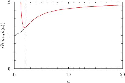
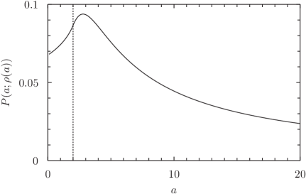
Figure 9: A plot of both $G(a,a;\rho(a))$ and $P(a;\rho(a))$. The dotted line indicates $a=2$. In the plot of $G(a,a;\rho(a))$ we have also marked the asymptotic form computed below.

Combining all of this information gives the phase diagram for our model, which we present in Figure 10. It is interesting to note that the three transition lines meet with the two critical lines forming an angle. Classically this would indicate mean-field like behaviour of a bicritical point. If true, this mean-field behaviour would be interesting to understand.

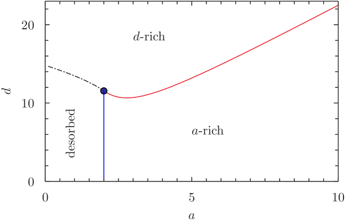
Figure 10: The phase diagram of our model. The three phases are as indicated and the first-order transition is marked with a dashed line, while the two second-order transitions are marked with solid lines. The three boundaries meet at the point $(a,d)=(2,11.55\dots)$.

6.6 Asymptotics of the $d$-rich-$a$-rich phase boundary

We now consider how the $d$-rich $a$-rich phase boundary, $d_{c}(a)$, behaves for large $a$ in more detail. From equation (5.4), we write $[z^{2n}a^{k}]G(a,a;z)$ in closed form

$$[z^{2n}a^{k}]G(a,a;z) =\frac{k(k+1)(k+2)}{(n+1)^{2}(n+2)(2n-k)}\binom{2n}{n}\binom{2n-k}{n}.$$ (6.23)

We seek the asymptotic form of $G(a,a;\rho(a))$ as $a\to\infty$, and so we need to evaluate the asymptotics of

$$G(a,a;\rho(a)) =\sum_{n\geq 0}\frac{(a-1)^{n}}{(n+1)^{2}(n+2)4^{n}a^{2n}}\binom{2n}{n}\sum_{k=0}^{n}\frac{k(k+1)(k+2)}{(2n-k)}\binom{2n-k}{n}a^{k}.$$ (6.24)

Expanding this slightly further gives

$$G(a,a;\rho(a)) =\sum_{n\geq 0}\frac{1}{(n+1)^{2}(n+2)4^{n}a^{2n}}\binom{2n}{n}\sum_{j,k=0}^{n}\frac{(-1)^{j}k(k+1)(k+2)}{(2n-k)}\binom{n}{j}\binom{2n-k}{n}a^{j+k}.$$ (6.25)

Substitute $$j=\ell-k$$ to get

$$=\sum_{n\geq 0}\frac{1}{(n+1)^{2}(n+2)4^{n}}\binom{2n}{n}\sum_{\ell=0}^{2n}a^{\ell-2n}\sum_{k=0}^{n}\frac{(-1)^{\ell-k}k(k+1)(k+2)}{(2n-k)}\binom{n}{\ell-k}\binom{2n-k}{n}.$$ (6.26)

So now the coefficient of $a^{0}$ is

$$[a^{0}] =\sum_{n=0}^{\infty}\frac{1}{n+1}\binom{2n}{n}4^{-n}=2,$$ (6.27)

while

$$[a^{-1}] =-\sum_{n=1}^{\infty}\frac{3n}{(n+1)(n+2)}\binom{2n}{n}4^{-n}=-2,$$ (6.28)

$$[a^{-2}] =0$$ (6.29)

$$[a^{-3}] =\sum_{n=2}^{\infty}\frac{2(n-1)}{(n+1)(n+2)}\binom{2n}{n}4^{-n}=1,$$ (6.30)

and

$$[a^{-4}] =\sum_{n=3}^{\infty}\frac{3(n-2)}{(n+1)(n+2)}\binom{2n}{n}4^{-n}=\frac{5}{4}.$$ (6.31)

These simple forms continue as far as we have observed. This then gives

$$G(a,a;\rho(a)) \sim 2-\frac{2}{a}+\frac{0}{a^{2}}+\frac{1}{a^{3}}+\frac{5}{4a^{4}}+\frac{15}{16a^{5}}+\frac{7}{32a^{6}}+O(a^{-7}).$$ (6.32)

We can then plot this against our numerical estimates of $G(a,a;\rho(a))$. One should note that the series $G(a,a,\rho(a))$ converges very slowly for $a>2$. Since we know the summands decay as $n^{-3/2}$, we can assume that the partial sums, $s_{n}$, grow as $A+Bn^{-1/2}$. We can then accelerate the convergence of the series by estimating $A$ with the sequence

$$A_{n} =s_{n}(n+\sqrt{n}\sqrt{n-1})-s_{n-1}(n-1+\sqrt{n}\sqrt{n-1}).$$ (6.33)

This combination was chosen by solving the pair of simultaneous equations $s_{n}=A+Bn^{-1/2},s_{n-1}=A+B(n-1)^{-1/2}$. We found that sequence $A_{n}$ converged far faster than the partial sums $s_{n}$.

7 Discussion

7.1 Nature of solution

In the section 6 we demonstrated that when $a=1$, the model undergoes a phase transition at $d=d_{c}(1)=\frac{8(512-165\pi)}{4096-1305\pi}$. Since this is not an algebraic number, it follows that the generating function of the model does not satisfy a linear differential equation in $z$ with integer polynomial coefficients in $a,d$ and $z$. That is, it cannot be D-finite.

Consider, to the contrary, that the generating function $G(1,d;z)=[r^{0}s^{0}]f(r,s;1,d;z)$ is a D-finite power series in $z$ with integer polynomial coefficients in $d$. By definition, it satisfies a non-trivial linear differential equation of the form

$$p_{k}(d;z)\frac{\partial^{k}G}{\partial{z}^{k}}+\dots p_{1}(d;z)\frac{\partial G}{\partial z}+p_{0}G(1,d;z) =0,$$ (7.1)

where the $p_{j}(d;z)$ are integer polynomials in $d$ and $z$. By standard results in the theory of linear differential equations, the singularities of $G(1,d;z)$ are zeros of the leading polynomial $p_{k}(d;z)$.

For small $d$ we know that the dominant singularity of $G(1,d)$ is $z_{b}=1/4$. At the critical value of $d$, there is a change in dominant singularity from $z_{b}$ to $z_{d}$. Exactly at the critical value, $z_{b}=z_{d}=1/4$. Thus the discriminant of $p_{k}(d;z)$ with respect to $d$ must be zero at this point. Since the discriminant is a polynomial in $z,d$ with integer coefficients and $z=1/4$, it follows that this critical value of $d$ must be an algebraic number. Above we showed that $d_{c}(1)=\frac{8(512-165\pi)}{4096-1305\pi}$ which is not algebraic and thus $G(1,d;z)$ is not D-finite. A standard result [38] on D-finite series states that specialisation of D-finite series are themselves D-finite and thus $G(a,d;z)$ cannot be D-finite and nor is $f(r,s;a,d;z)$.

The Lindström-Gessel-Viennot lemma combines the partition functions of single-walk models — equivalent to sums and Hadamard products of the underlying single-walk generating function which is algebraic (this is true quite generally — see [39]). Any finite combination of Hadamard products and sums of algebraic or D-finite generating functions remains D-finite [38] and thus the Lindström-Gessel-Viennot lemma (alone) cannot be applied to decompose the model considered here into single-walk problems.

That being said, the Lindström-Gessel-Viennot lemma can be combined with a factorisation argument to yield a solution as we demonstrated in section 5.

7.2 Fixed energy ratio models: $r$-models

Finally, let us now consider the family of physical models parameterised by $-\infty<r<\infty$ where

$$\varepsilon_{d} =r\varepsilon_{a} d =a^{r}$$ and so (7.2)

that allows us to summarise our results. Let us call these $r$-models.

For any $r$-model the high temperature phase is the desorbed state. The model effectively already analysed by Brak et al. [36, 37] has $d=a$ and so $r=1$. In this case there is a single low temperature phase being the $a$-rich phase. Given there are no additional phase boundaries for $a<d$ one can deduce that for all $r\leq 1$ the model goes from the desorbed state at high temperatures through a single second-order phase transition to the $a$-rich phase at low temperatures.

The special point in our phase diagram where $(a,d)=(2,11.55\ldots)$ where the three phases meet occurs in the $r$-model with

$$r=r_{t}\equiv\frac{\log(11.55\ldots)}{\log{2}}=3.53\ldots.$$ (7.3)

For all $r\geq r_{t}$ there is a single low temperature phase which is the $d$-rich phase: the transition on lowering the temperature is now first-order.

Since we have shown above that $d_{c}(a)\sim 2a$ as $a\rightarrow\infty$ one can now argue that for all $1<r<r_{t}$ the $r$-model has two phase transitions on lowering the temperature. At very low temperatures the model is in a $d$-rich phase while at high temperatures the model is in the desorbed state. At intermediate temperatures the system is in an $a$-rich phase. Both transitions, from desorbed to $a$-rich, and $a$-rich to $d$-rich, are second-order transitions with jump discontinuities in the specific heat. In Figure 11 we plot the fluctuations in $a$-visits as a function of temperature at length 128 for the $r=2$ $r$-model: two peaks occur in these fluctuations.

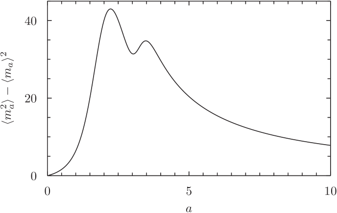
Figure 11: A plot of the fluctuations in the number of $a$-visits, $m_{a}$, for length $n=128$ as function of $a$ clearly showing two peaks.

If one argues that a physically realisable model is one where both walks pick up the same energy when they touch the surface together then the model is the one with $r=2$, that is $d=a^{2}$. It is interesting to see that this model contains two phase transitions: one at $a=2$ and the other at $a\approx 3.301$ found by solving equation (6.20) for $d_{c}=a_{c}^{2}$. In any case, we have a family of adsorption models that have one or two low temperature states and which the order of the transition changes as the parameter is varied. We have analysed this model using an exact solution and fully delineated its behaviour. It will be of interest to analyse the behaviour of this model in a slit.

References

- [1] V. Privman, G. Forgacs, and H. L. Frisch, Phys. Rev. B 37, 9897 (1988).
- [2] K. DeBell and T. Lookman, Rev. Mod. Phys. 65, 87 (1993).
- [3] E. J. Janse van Rensburg, The Statistical Mechanics of Interacting Walks, Polygons, Animals and Vesicles, Oxford University Press, Oxford, 2000.
- [4] P. K. Mishra, S. Kumar, and Y. Singh, Physica A 323, 453 (2003).
- [5] R. Brak, A. L. Owczarek, A. Rechnitzer, and S. Whittington, J. Phys. A 38, 4309 (2005).
- [6] E. J. Janse van Rensburg, E. Orlandini, A. L. Owczarek, A. Rechnitzer, and S. Whittington, J. Phys. A 38, L823 (2005).
- [7] R. Martin, E. Orlandini, A. L. Owczarek, A. Rechnitzer, and S. Whittington, J. Phys. A 40, 7509 (2007).
- [8] A. L. Owczarek, R. Brak, and A. Rechnitzer, J. Math. Chem. 45, 113 (2008).
- [9] J. Alvarez, E. J. Janse van Rensburg, C. E. Soteros, and S. G. Whittington, J. Phys. A.: Math. and Theor. 41, 185004 (2008).
- [10] A. Owczarek, J. Stat. Mech.: Theor. Exp. , P11002:1 (2009).
- [11] E. J. Janse van Rensburg, J. Stat. Mech: Theor. Exp. , P08030 (2010).
- [12] G. Rychlewski and S. G. Whittington, J. Phys. A.: Math. Theor. 41, 095006 (2011).
- [13] K. Svoboda and S. M. Block, Ann. Rev. Biophys. Biomol. Struct. 23, 247 (1994).
- [14] A. Ashkin, Proc. Natl. Acad. Sci. USA 94, 4853 (1997).
- [15] T. Strick, J.-F. Allemand, V. Croquette, and D. Bensimon, Phys. Today 54, 46 (2001).
- [16] B. Essevaz-Roulet, U. Bockelmann, and F. Heslot, Proc. Natl. Acad. Sci. USA 94, 11935 (1997).
- [17] D. K. Lubensky and D. R. Nelson, Phys. Rev. Lett. 85, 1572 (2002).
- [18] D. K. Lubensky and D. R. Nelson, Phys. Rev. E 65, 031917 (2002).
- [19] E. Orlandini, S. M. Bhattacharjee, D. Marenduzzo, A. Maritan, and F. Seno, J. Phys. A: Math. Gen. 34, L751 (2001).
- [20] D. Marenduzzo, A. Trovato and A. Maritan, Phys. Rev. E 64, 031901 (2001).
- [21] D. Marenduzzo, S. M. Bhattacharjee, A. Maritan, E. Orlandini, and F. Seno, Phys. Rev. Lett. 88, 028102 (2002).
- [22] D. Marenduzzo, A. Maritan, A. Rosa, and F. Seno, Phys. Rev. Lett. 90, 088301 (2003).
- [23] D. Marenduzzo, A. Maritan, A. Rosa, and F. Seno, J. Stat. Mech. , L04001 (2009).
- [24] P.-G. de Gennes, Scaling Concepts in Polymer Physics, Cornell University Press, Ithaca, 1979.
- [25] R. Hegger and P. Grassberger, J. Phys. A. 27, 4069 (1994).
- [26] E. J. Janse van Rensburg and A. Rechnitzer, J. Phys. A 37, 13869 (2004).
- [27] D. Poland and H.A. Scheraga, Theory of helix-coil transitions in biopolymers, Academic Press, 1970.
- [28] C. Richard and A.J. Guttmann, J. Stat. Phys. 115, 925, (2004).
- [29] R. Kapri, J. Chem. Phys. 130, 145105, (2009).
- [30] A. L. Owczarek, A. Rechnitzer and R. Tabbara, In preparation.
- [31] I. M. Gessel and X. Viennot, Advances in Mathematics 58, 300 (1985).
- [32] B. Lindström, Bull. London. Math. Soc. 5, 85 (1973).
- [33] S. Karlin and G. McGregor, Pacific Journal of Mathematics 9, 1141 (1959).
- [34] M. Bousquet-Mélou and M. Mishna, Contemp. Math 520, 1 (2010).
- [35] P. Flajolet and R. Sedgewick, Analytic combinatorics, Cambridge Univ Pr, 2009.
- [36] R. Brak, J. Essam, and A. L. Owczarek, J. Stat. Phys. 93, 155 (1998).
- [37] A. L. Owczarek, J. Essam, and R. Brak, J. Stat. Phys. 102, 997 (2001).
- [38] L. Lipshitz, Journal of Algebra (1989).
- [39] M. Bousquet-Mélou, Séminaire Lotharingien de Combinatoire 57, 23 (2008).