Fermionic vacuum polarization by a flat boundary
in cosmic string spacetime

Abstract

In this paper we investigate the fermionic condensate and the renormalized vacuum expectation value (VEV) of the energy-momentum tensor for a massive fermionic field induced by a flat boundary in the cosmic string spacetime. In this analysis we assume that the field operator obeys MIT bag boundary condition on the boundary. We explicitly decompose the VEVs into the boundary-free and boundary-induced parts. General formulas are provided for both parts which are valid for any value of the parameter associated with the cosmic string. For a massless field, the boundary-free part in the fermionic condensate and the boundary-induced part in the energy-momentum tensor vanish. For a massive field the radial stress is equal to the energy density for both boundary-free and boundary-induced parts. The boundary-induced part in the stress along the axis of the cosmic string vanishes. The total energy density is negative everywhere, whereas the effective pressure along the azimuthal direction is positive near the boundary and negative near the cosmic string. We show that for points away from the boundary, the boundary-induced parts in the fermionic condensate and in the VEV of the energy-momentum tensor vanish on the string.

PACS numbers: 03.70.+k, 98.80.Cq, 11.27.+d

1 Introduction

Non-trivial structure of the vacuum state is among the most profound predictions of quantum field theory. The properties of the vacuum are manifested in its response to different external perturbations. The imposition of boundary conditions on a quantum field is among the simplest models for the perturbation. The boundary conditions may be induced by real material media or represent non-trivial topology of the space. In both cases they modify the structure of the quantum vacuum thus affecting the vacuum expectation values (VEVs) of physical observables. This phenomenon is known as the Casimir effect (for reviews see Ref. [1]). In the present paper we consider combined effects from boundaries and non-trivial topology on the properties of the fermionic vacuum in the cosmic string spacetime.

The cosmic strings are predicted to be formed within the framework of grand unified theories as a result of symmetry braking phase transitions [2]. This type of phase transitions have several cosmological consequences and provide an important link between particle physics and cosmology. Although the recent observational data on the cosmic microwave background radiation have ruled out cosmic strings as the primary source for primordial density perturbations, they are still candidates for the generation of a number of interesting physical effects such as the generation of gravitational waves, gamma ray bursts, high energy cosmic rays, and enhanced baryon number violation. Recently, cosmic strings attracted a renewed interest partly because a variant of their formation mechanism is proposed in the framework of brane inflation [3] (for a review of the existence of cosmic strings in string theory models see [4]).

At distances larger than the core radius, the spacetime geometry for a straight cosmic string is well approximated by a flat spacetime with a planar angle deficit. In quantum field theory, the corresponding non-trivial topology gives rise to the polarization of the quantum vacuum. This problem has been studied in many papers for scalar, fermionic and electromagnetic fields [5]-[31]. The vacuum polarization by a cosmic string in various curved backgrounds has been discussed in [32, 33, 34, 35]. Another type of vacuum polarization arises by the presence of boundaries on which the field operator obeys some prescribed boundary condition. The analysis of the boundary-induced quantum effects in the cosmic string spacetime have been developed for scalar [36, 37], fermionic [38, 39], and electromagnetic fields [37, 40, 41] for the geometry of a coaxial cylindrical boundary. From the point of view of the physics in the exterior region, the latter can be considered as a simplified model for the nontrivial core of the cosmic string. The Casimir force for massless scalar fields subject to Dirichlet and Neumann boundary conditions in the setting of the conical piston has been recently investigated in [42]. The Casimir densities for scalar and electromagnetic fields induced by flat boundaries perpendicular to the string have been considered in [43, 44]. The topological effects in the generalized cosmic string geometry with a compact dimension along its axis are investigated in [45]. Combined effects of topology and boundaries on the Casimir-Polder force acting on a polarizable microparticle situated near the cosmic string have been studied in [46]. In particular, it has been shown that due to the nontrivial topology this force can be repulsive.

Continuing in this line of investigations, in the present paper we consider the polarization of the fermionic vacuum by a flat boundary perpendicular to the string axis on which the field operator is constrained by MIT bag boundary condition. We evaluate the fermionic condensate (FC) and the VEV of the energy-momentum tensor. These quantities are among the most important characteristics of the vacuum state. Although the corresponding operators are local, they carry an important information about the global properties of the background spacetime. In addition to describing the physical structure of the quantum field at a given point, the energy-momentum tensor acts as the source in Einstein’s equations and, therefore, it plays an important role in modelling a self-consistent dynamics which involves the gravitational field. The FC is crucial in the models of dynamical chiral symmetry breaking and in considerations of the stability of fermionic vacuum. As it will be shown below, in the problem under consideration all calculations can be performed in a closed form and it constitutes an example in which the topological and boundary-induced polarizations of the vacuum can be separated in different contributions. Note that a conical space appears as an effective background geometry in the long-wavelength description of certain condensed matter systems such as crystals, liquid crystals and quantum liquids [47]. The results described in this paper may shed light on the features of the boundary-induced effects in this type of medium with a conical defect.

The rest of the paper is organized as follows. In the next section we describe the geometry of the problem and a complete set of positive- and negative-energy four-spinors obeying the bag boundary condition on the plate is constructed. In section 3 these mode functions are applied for the evaluation of the FC. Similar calculations for the VEV of the energy-momentum tensor are presented in section 4. The main results of the paper are summarized in section 5. The technical details for the evaluation of the energy density and the azimuthal stress are described in Appendix A.

2 Geometry of the problem and mode functions

We consider the background spacetime corresponding to an infinitely long straight cosmic string. Considering the string along the $z$-axis, by using cylindrical coordinates the line element associated with this spacetime reads:

$$ds^{2}=dt^{2}-dr^{2}-r^{2}d\phi^{2}-dz{}^{2},$$ (2.1)

where $0\leqslant\phi\leqslant\phi_{0}=2\pi/q$ and the spatial points $(r,\phi,z)$ and $(r,\phi+\phi_{0},z)$ are to be identified. The line element (2.1) has been derived in [48] in the weak-field approximation. In this case, the planar angle deficit is related to the mass per unit length of the string, $\mu_{0}$, by $2\pi-\phi_{0}=8\pi G\mu_{0}$, where $G$ is the Newton gravitational constant. The validity of the line element (2.1) has been extended beyond linear perturbation theory by several authors [49] (see also [2]). In this case, the parameter $q$ need not to be close to 1. This is the case also in condensed matter systems with conical defects. For example, in graphitic cones one has $q=6/5,3/2,2,3,6$. All this type of cones have been experimentally observed [50].

The dynamics of a massive fermionic field in curved spacetime with the metric tensor $g^{\mu\nu}$ is governed by the Dirac equation

$$i\gamma^{\mu}\nabla_{\mu}\psi-m\psi=0\ ,$$ (2.2)

with the covariant derivative operator

$$\nabla_{\mu}=\partial_{\mu}+\Gamma_{\mu}\ ,\quad\Gamma_{\mu}=\gamma^{\nu}\gamma_{\nu;\mu}/4\ .$$ (2.3)

Here $\gamma^{\mu}$ are the Dirac matrices in curved spacetime and $\Gamma_{\mu}$ is the spin connection. Here and below, $\mu=0,1,2,3$ correspond to the coordinates $t,r,\phi,z$, respectively, and the semicolon means the standard covariant derivative for vector fields.

In the present paper we are interested in quantum vacuum effects induced by a flat boundary located at $z=0$. We assume that on the boundary the field operator obeys MIT bag boundary condition:

$$\left(1+i\gamma^{\mu}n_{\mu}\right)\psi=0\ ,\quad z=0,$$ (2.4)

where $n_{\mu}$ is the outward-pointing normal to the boundary. In the discussion below we will consider the region $z>0$ with $n_{\mu}=(0,0,0,-1)$. For the evaluation of the VEVs we will use the direct mode summation procedure. In this approach one needs to have the complete set of the eigenfunctions satisfying boundary condition (2.4).

In the discussion below the gamma matrices will be taken in the Dirac representation:

$$\gamma^{0}=\left(\begin{array}[]{cc}1&0\\ 0&-1\end{array}\right),\;\gamma^{l}=\left(\begin{array}[]{cc}0&\beta^{l}\\ -\beta^{l}&0\end{array}\right),$$ (2.5)

with $\beta^{l}$, $l=1,2,3$, being the Pauli matrices in cylindrical coordinates with a planar angle deficit:

$$\beta^{1}=\left(\begin{array}[]{cc}0&e^{-iq\phi}\\ e^{iq\phi}&0\end{array}\right),\;\beta^{2}=-\frac{i}{r}\left(\begin{array}[]{cc}0&e^{-iq\phi}\\ -e^{iq\phi}&0\end{array}\right),$$

and $\beta^{3}=\mathrm{diag}(1,-1)$. We have the standard anticommutation relation $\beta^{l}\beta^{n}+\beta^{n}\beta^{l}=-2g^{ln}$. For the spin connection one gets

$$\Gamma_{\mu}=\frac{1-q}{2}r\gamma^{1}\gamma^{2}\delta_{\mu}^{2}.$$ (2.6)

By taking into account that $\gamma^{\mu}\Gamma_{\mu}=(1-q)\gamma^{1}/(2r)$, the Dirac equation takes the form

$$\gamma^{\mu}\partial_{\mu}\psi+\frac{1-q}{2r}\gamma^{1}\psi+im\psi=0.$$ (2.7)

First we consider the positive-energy solutions of this equation obeying the boundary condition (2.4).

2.1 Positive-energy modes

For the positive-energy solutions the time dependence has the form $e^{-i\omega t}$. Decomposing the four-spinor $\psi$ into two-component spinors,

$$\psi=\left(\begin{array}[]{c}\varphi\\ \chi\end{array}\right),$$ (2.8)

from Eq. (2.7) for the upper and lower components we find the set of equations

$$\left(\beta^{l}\partial_{l}\mathbf{+}\frac{1-q}{2r}\beta^{1}\right)\varphi-i\left(\omega+m\right)\chi = 0,$$

$$\left(\beta^{l}\partial_{l}\mathbf{+}\frac{1-q}{2r}\beta^{1}\right)\chi-i\left(\omega-m\right)\varphi = 0,$$ (2.9)

From (2.9) the following equation is obtained for the upper component:

$$\left[-g^{ij}\partial_{i}\partial_{j}\mathbf{+}\frac{1}{r}\partial_{1}+\frac{q-1}{r}\beta^{1}\beta^{2}\partial_{2}\mathbf{-}\frac{(q-1)^{2}}{4r^{2}}+\omega^{2}-m^{2}\right]\varphi=0,$$ (2.10)

where $i,j=1,2,3$.

Further decomposing the two-spinor $\varphi$ as

$$\varphi=\left(\begin{array}[]{c}\varphi_{1}\\ \varphi_{2}\end{array}\right),$$ (2.11)

we can present the solutions for the separate components in the form

$$\varphi_{l}=f_{l}(r)\left(C_{\varphi 1}^{(l)}e^{ikz}+C_{\varphi 2}^{(l)}e^{-ikz}\right)e^{i\left(qn_{l}\phi-\omega t\right)},\;l=1,2,$$ (2.12)

with $0\leqslant k<\infty$ and $n_{l}=0,\pm 1,\pm 2,\ldots$. Substituting (2.12) into (2.10), we can see that for the radial functions the Bessel equation is obtained with the solutions regular at the string $f_{l}(r)=J_{\beta_{l}}(\lambda r)$, where

$$\beta_{l}=|qn_{l}-(-1)^{l}(q-1)/2|,$$ (2.13)

and $\lambda=\sqrt{\omega^{2}-k^{2}-m^{2}}$. By using (2.12), for the components of the lower two-spinor,

$$\chi=\left(\begin{array}[]{c}\chi_{1}\\ \chi_{2}\end{array}\right),$$ (2.14)

we get

$$\chi_{l}=J_{\beta_{l}}(\lambda r)\left(B_{\varphi 1}^{(l)}e^{ikz}+B_{\varphi 2}^{(l)}e^{-ikz}\right)e^{i\left(qn_{l}\phi-\omega t\right)},$$ (2.15)

with the relations $n_{2}=n_{1}+1$, $\beta_{2}=\beta_{1}+\epsilon_{n_{1}}$, and we have defined

$$\epsilon_{n_{1}}=\left\{\begin{array}[]{cc}1,&n_{1}\geqslant 0\\ -1,&n_{1}<0\end{array}\right..$$ (2.16)

The coefficients in (2.15) are defined by the expressions

$$B_{\varphi 1}^{(1)} = \frac{kC_{\varphi 1}^{(1)}-i\lambda\epsilon_{n_{1}}C_{\varphi 1}^{(2)}}{\omega+m},\;B_{\varphi 2}^{(1)}=-\frac{kC_{\varphi 2}^{(1)}+i\lambda\epsilon_{n_{1}}C_{\varphi 2}^{(2)}}{\omega+m},$$

$$B_{\varphi 1}^{(2)} = -\frac{kC_{\varphi 1}^{(2)}-i\lambda\epsilon_{n_{1}}C_{\varphi 1}^{(1)}}{\omega+m},\;B_{\varphi 2}^{(2)}=\frac{kC_{\varphi 2}^{(2)}+i\lambda\epsilon_{n_{1}}C_{\varphi 2}^{(1)}}{\omega+m}.$$ (2.17)

Hence, the positive-energy solution to the Dirac equation has the form ($n_{1}=n$)

$$\psi_{\sigma}^{(+)}=\left(\begin{array}[]{c}\left(C_{\varphi 1}^{(1)}e^{ikz}+C_{\varphi 2}^{(1)}e^{-ikz}\right)J_{\beta}(\lambda r)\\ \left(C_{\varphi 1}^{(2)}e^{ikz}+C_{\varphi 2}^{(2)}e^{-ikz}\right)J_{\beta+\epsilon_{n}}(\lambda r)e^{iq\phi}\\ \left(B_{\varphi 1}^{(1)}e^{ikz}+B_{\varphi 2}^{(1)}e^{-ikz}\right)J_{\beta}(\lambda r)\\ \left(B_{\varphi 1}^{(2)}e^{ikz}+B_{\varphi 2}^{(2)}e^{-ikz}\right)J_{\beta+\epsilon_{n}}(\lambda r)e^{iq\phi}\end{array}\right)e^{i\left(qn\phi-\omega t\right)},$$ (2.18)

where

$$\beta=|q(n+1/2)-1/2|,$$ (2.19)

and $\sigma$ is a collective notation for the set of quantum numbers specifying the solution (see below). We can see that the four-spinor $\psi_{\sigma}^{(+)}$ is an eigenfunction of the projection of the total momentum along the cosmic string:

$$\widehat{J}_{3}\psi_{\sigma}^{(+)}=\left(-i\partial_{\phi}+i\frac{q}{2}r\gamma^{1}\gamma^{2}\right)\psi_{\sigma}^{(+)}=qj\psi_{\sigma}^{(+)},$$ (2.20)

with

$$j=n+1/2.$$ (2.21)

Note that $\epsilon_{j}=\epsilon_{n}$.

Now we impose the boundary condition (2.4) on the four-spinor (2.18). From this condition the following two equations are obtained for the upper and lower components:

$$\varphi_{1}-i\chi_{1}=0,\;\varphi_{2}+i\chi_{2}=0\;\text{at}\;z=0.$$ (2.22)

By using these relations, the coefficients in (2.18) are expressed in terms of $C_{\varphi 1}^{(1)}$ and $C_{\varphi 2}^{(1)}$ as

$$C_{\varphi 1}^{(2)} = \frac{\epsilon_{n}}{ik\lambda}\left\{\left[k^{2}+m\left(\omega+m\right)\right]C_{\varphi 1}^{(1)}+\left(\omega+m\right)\left(m+ik\right)C_{\varphi 2}^{(1)}\right\},$$

$$C_{\varphi 2}^{(2)} = -\frac{\epsilon_{n}}{ik\lambda}\left\{\left(\omega+m\right)\left(m-ik\right)C_{\varphi 1}^{(1)}+\left[k^{2}+m\left(\omega+m\right)\right]C_{\varphi 2}^{(1)}\right\},$$ (2.23)

and

$$B_{\varphi 1}^{(1)} = -\frac{m}{k}C_{\varphi 1}^{(1)}-\left(\frac{m}{k}+i\right)C_{\varphi 2}^{(1)},$$

$$B_{\varphi 2}^{(1)} = \left(\frac{m}{k}-i\right)C_{\varphi 1}^{(1)}+\frac{m}{k}C_{\varphi 2}^{(1)},$$

$$B_{\varphi 1}^{(2)} = i\frac{\epsilon_{n}}{\lambda}\left[\omega C_{\varphi 1}^{(1)}+\left(m+ik\right)C_{\varphi 2}^{(1)}\right],$$

$$B_{\varphi 2}^{(2)} = i\frac{\epsilon_{n}}{\lambda}\left[\left(m-ik\right)C_{\varphi 1}^{(1)}+\omega C_{\varphi 2}^{(1)}\right].$$ (2.24)

One of the coefficients $C_{\varphi 1}^{(1)}$ and $C_{\varphi 2}^{(1)}$ is determined from the normalization condition obeyed by the wave function and, hence, one coefficient remains arbitrary. In order to determine the latter some additional condition should be imposed. A similar situation to find fermionic wave function was present for the problem with cylindrical boundary [38]. However, as it can be seen, the additional condition used there is not appropriate for the present case.

In order to specify the second constant we impose the condition

$$B_{\varphi 2}^{(2)}/B_{\varphi 1}^{(2)}=-C_{\varphi 2}^{(1)}/C_{\varphi 1}^{(1)}.$$ (2.25)

By taking into account Eq. (2.24), this leads to the following relation

$$C_{\varphi 2}^{(1)}=i\kappa_{s}C_{\varphi 1}^{(1)},$$ (2.26)

where we have defined

$$\kappa_{s}=\frac{\omega+s\lambda}{k-im},\;s=\pm 1.$$ (2.27)

Note that we have the relation $\kappa_{s}\kappa_{-s}^{\ast}=1$.

With the relation (2.26) all coefficients are expressed in terms of $C_{\varphi 1}^{(1)}$. Introducing the notations

$$f_{\pm}(z) = e^{ikz}\pm i\kappa_{s}e^{-ikz},$$

$$g_{\pm}(z) = \left(\omega\pm m\right)f_{\pm}(z)+s\lambda f_{\mp}(z),$$ (2.28)

the positive-energy solutions are written in the form

$$\psi_{\sigma}^{(+)}=C_{\varphi 1}^{(1)}\left(\begin{array}[]{c}f_{+}(z)J_{\beta}(\lambda r)e^{-iq\phi/2}\\ i\frac{\epsilon_{j}s}{k}g_{+}(z)J_{\beta+\epsilon_{j}}(\lambda r)e^{iq\phi/2}\\ \frac{1}{k}g_{-}(z)J_{\beta}(\lambda r)e^{-iq\phi/2}\\ -i\epsilon_{j}sf_{-}(z)J_{\beta+\epsilon_{j}}(\lambda r)e^{iq\phi/2}\end{array}\right)e^{i\left(qj\phi-\omega t\right)},$$ (2.29)

where $j=\pm 1/2,\pm 3/2,\ldots$, and

$$\beta=\beta_{1}=q|j|-\epsilon_{j}/2.$$ (2.30)

Now the set of quantum numbers is specified to $\sigma=(\lambda,k,j,s)$ and

$$\omega=\sqrt{\lambda^{2}+k^{2}+m^{2}}.$$ (2.31)

It can be checked that the mode functions (2.29) are orthogonal: $\int d^{3}x\sqrt{|g|}\psi_{\sigma}^{(+)+}\psi_{\sigma^{\prime}}^{(+)}=0$ for $\sigma\neq\sigma^{\prime}$. The remained coefficient $C_{\varphi 1}^{(1)}$ is found from the normalization condition

$$\int d^{3}x\sqrt{|g|}\psi_{\sigma}^{(+)+}\psi_{\sigma^{\prime}}^{(+)}=\delta(\lambda^{\prime}-\lambda)\delta(k^{\prime}-k)\delta_{j^{\prime}j}\delta_{s^{\prime}s}\ .$$ (2.32)

By taking into account that

$$\int_{0}^{\infty}drrJ_{\beta}(\lambda r)J_{\beta}(\lambda^{\prime}r)=\frac{1}{\lambda}\delta(\lambda-\lambda^{\prime}),$$ (2.33)

we find

$$|C_{\varphi 1}^{(1)}|^{2}=\frac{k^{2}\lambda}{8\pi\phi_{0}\omega(\omega+s\lambda)}.$$ (2.34)

It can be seen that, the positive-energy mode functions (2.29), with the normalization coefficient given by (2.34), are invariant, up to a phase, with respect to the transformation $(k,s)\rightarrow(-k,-s)$.

2.2 Negative-energy modes

The time-dependence of the negative-energy mode function is in the form $e^{i\omega t}$. For the lower two-spinor, $\chi$, we obtain the same equation as in (2.10). For the corresponding upper and lower components one finds

$$\chi_{l}=J_{\beta_{l}}(\lambda r)(C_{\chi 1}^{(l)}e^{ikz}+C_{\chi 2}^{(l)}e^{-ikz})e^{i\left(qn_{l}\phi+\omega t\right)},\;l=1,2,$$ (2.35)

with the notations (2.13). Substituting these expressions into (2.9), for the upper components we find the expressions

$$\varphi_{l}=(B_{\chi 1}^{(l)}e^{ikz}+B_{\chi 2}^{(l)}e^{-ikz})J_{\beta_{l}}(\lambda r)e^{i\left(qn_{l}\phi+\omega t\right)},$$ (2.36)

and the relations $n_{2}=n_{1}+1$, $\beta_{2}=\beta_{1}+\epsilon_{n_{1}}$. Denoting $n_{1}=n$, the coefficients in (2.36) are given by the expressions

$$B_{\chi 1}^{(1)} = -\frac{kC_{\chi 1}^{(1)}-i\lambda\epsilon_{n}C_{\chi 1}^{(2)}}{\omega+m},\;B_{\chi 2}^{(1)}=\frac{kC_{\chi 2}^{(1)}+i\lambda\epsilon_{n}C_{\chi 2}^{(2)}}{\omega+m},$$

$$B_{\chi 1}^{(2)} = \frac{kC_{\chi 1}^{(2)}-i\lambda\epsilon_{n}C_{\chi\varphi 1}^{(1)}}{\omega+m},\;B_{\chi 2}^{(2)}=-\frac{kC_{\chi 2}^{(2)}+i\lambda\epsilon_{n}C_{\chi\varphi 2}^{(1)}}{\omega+m}.$$ (2.37)

As a result, he negative energy modes are presented as

$$\psi_{\sigma}^{(-)}=\left(\begin{array}[]{c}(B_{\chi 1}^{(1)}e^{ikz}+B_{\chi 2}^{(1)}e^{-ikz})J_{\beta}(\lambda r)\\ (B_{\chi 1}^{(2)}e^{ikz}+B_{\chi 2}^{(2)}e^{-ikz})J_{\beta+\epsilon_{n}}(\lambda r)e^{iq\phi}\\ (C_{\chi 1}^{(1)}e^{ikz}+C_{\chi 2}^{(1)}e^{-ikz})J_{\beta}(\lambda r)\\ (C_{\chi 1}^{(2)}e^{ikz}+C_{\chi 2}^{(2)}e^{-ikz})J_{\beta+\epsilon_{n}}(\lambda r)e^{iq\phi}\end{array}\right)e^{i\left(qn\phi+\omega t\right)},$$ (2.38)

with $\beta$ defined in (2.19).

From the boundary conditions (2.22) the coefficients are expressed in terms of $C_{\chi 1}^{(1)}$ and $C_{\chi 2}^{(1)}$:

$$C_{\chi 1}^{(2)} = \frac{\epsilon_{n}}{ik\lambda}\left\{\left[k^{2}+m\left(\omega+m\right)\right]C_{\chi 1}^{(1)}+\left(\omega+m\right)\left(m+ik\right)C_{\chi 2}^{(1)}\right\},$$

$$C_{\chi 2}^{(2)} = -\frac{\epsilon_{n}}{ik\lambda}\left\{\left(\omega+m\right)\left(m-ik\right)C_{\chi 1}^{(1)}+\left[k^{2}+m\left(\omega+m\right)\right]C_{\chi 2}^{(1)}\right\},$$ (2.39)

and

$$B_{\chi 1}^{(1)} = \frac{m}{k}C_{\chi 1}^{(1)}+\left(\frac{m}{k}+i\right)C_{\chi 2}^{(1)},$$

$$B_{\chi 2}^{(1)} = -\left(\frac{m}{k}-i\right)C_{\chi 1}^{(1)}-\frac{m}{k}C_{\chi 2}^{(1)},$$

$$B_{\chi 1}^{(2)} = \frac{\epsilon_{n}}{i\lambda}\left[\omega C_{\chi 1}^{(1)}+\left(m+ik\right)C_{\chi 2}^{(1)}\right],$$

$$B_{\chi 2}^{(2)} = \frac{\epsilon_{n}}{i\lambda}\left[\left(m-ik\right)C_{\chi 1}^{(1)}+\omega C_{\chi 2}^{(1)}\right].$$ (2.40)

Similar to the case of positive-energy modes, an additional condition should be imposed. As such a condition we impose

$$B_{\chi 2}^{(2)}/B_{\chi 1}^{(2)}=-C_{\chi 2}^{(1)}/C_{\chi 1}^{(1)}.$$ (2.41)

Taking into account (2.40), this gives

$$C_{\chi 2}^{(1)}=i\kappa_{s}C_{\chi 1}^{(1)},\;s=\pm 1,$$ (2.42)

with $\kappa_{s}$ defined in (2.27).

As a result, the negative-energy mode functions are written in the form

$$\psi_{\sigma}^{(-)}=C_{\chi 1}^{(1)}\left(\begin{array}[]{c}-\frac{1}{k}g_{-}(z)J_{\beta}(\lambda r)e^{-iq\phi/2}\\ i\epsilon_{j}sf_{-}(z)J_{\beta+\epsilon_{j}}(\lambda r)e^{iq\phi/2}\\ f_{+}(z)J_{\beta}(\lambda r)e^{-iq\phi/2}\\ i\frac{\epsilon_{j}s}{k}g_{+}(z)J_{\beta+\epsilon_{j}}(\lambda r)e^{iq\phi/2}\end{array}\right)e^{i\left(qj\phi+\omega t\right)},$$ (2.43)

with the same notations as in (2.29). The function is an eigenfunction for the projection of the total angular momentum on the $z$-axis, $\widehat{J}_{3}\psi_{\sigma}^{(-)}=qj\psi_{\sigma}^{(-)}$, and we have introduced the related quantum number $j=n+1/2$. It can be checked that the modes (2.43) obey the orthogonality relations $\int d^{3}x\sqrt{|g|}\psi_{\sigma^{\prime}}^{(\pm)+}\psi_{\sigma}^{(-)}=0$ for $\sigma\neq\sigma^{\prime}$. From the normalization condition we can see that $|C_{\chi 1}^{(1)}|^{2}=|C_{\varphi 1}^{(1)}|^{2}$. Note that we have a correspondence between the negative- and positive-energy modes given by the relation (up to a phase)

$$\psi_{\sigma}^{(-)}e^{-i\omega t}=\gamma^{5}\gamma^{0}\psi_{\sigma}^{(+)}e^{i\omega t},$$ (2.44)

where in cylindrical coordinates $\gamma^{5}=ir\gamma^{0}\gamma^{1}\gamma^{2}\gamma^{3}$. This relation corresponds to the PCT transformation of four-spinors.

The wave functions obtained in this section can be used for the investigation of various quantum electrodynamics effects around the cosmic string in the presence of boundary involving electrons and positrons (for example, bremsstrahlung and electron-positron pair production by a photon). In what follows we use these functions for the evaluation of the FC and the VEV of the energy-momentum tensor.

3 Fermionic condensate

Having the complete set of mode functions for the fermionic field, we can evaluate the effects of the boundary on the FC, $\langle 0|\bar{\psi}\psi|0\rangle$, where $|0\rangle$ is the vacuum state in the geometry of a cosmic string with flat boundary and $\bar{\psi}=\psi^{+}\gamma^{0}$ is the Dirac adjoint. Expanding the field operator in terms of the complete set $\{\psi_{\sigma}^{(-)},\psi_{\sigma}^{(+)}\}$ and by using the definition of the vacuum state, the following formula is obtained for the condensate:

$$\langle 0|\bar{\psi}\psi|0\rangle=\sum_{\sigma}\bar{\psi}_{\sigma}^{(-)}\psi_{\sigma}^{(-)},$$ (3.1)

where

$$\sum_{\sigma}=\sum_{s=\pm 1}\sum_{j=\pm 1/2,\ldots}\int_{0}^{\infty}d\lambda\int_{0}^{\infty}dk.$$ (3.2)

Substituting (2.43) into (3.1), the expression obtained is divergent and some regularization procedure is needed. We will assume that a cutoff function is present without explicitly writing it. The specific form of this function will not be important for the further discussion.

By making use of the expression (2.43) for the mode functions and the relation

$$\sum_{j=\pm 1/2,\ldots}J_{\beta}^{2}(\lambda r)=\sum_{j=\pm 1/2,\ldots}J_{\beta+\epsilon_{j}}^{2}(\lambda r)=\sum_{j}\left[J_{qj-1/2}^{2}(\lambda r)+J_{qj+1/2}^{2}(\lambda r)\right],$$ (3.3)

the FC is presented in the form

$$\langle 0|\bar{\psi}\psi|0\rangle=\langle 0|\bar{\psi}\psi|0\rangle_{\mathrm{s}}+\langle\bar{\psi}\psi\rangle_{\mathrm{b}}.$$ (3.4)

Here the separate terms on the right-hand side are given by the expressions

$$\langle 0|\bar{\psi}\psi|0\rangle_{\mathrm{s}}=-\frac{qm}{\pi^{2}}\sum_{j}\int_{0}^{\infty}d\lambda\int_{0}^{\infty}dk\frac{\lambda}{\omega}[J_{qj-1/2}^{2}(\lambda r)+J_{qj+1/2}^{2}(\lambda r)],$$ (3.5)

and

$$\langle\bar{\psi}\psi\rangle_{\mathrm{b}} = \frac{iq}{2\pi^{2}}\sum_{j}\int_{0}^{\infty}d\lambda\int_{0}^{\infty}dk\frac{\lambda}{\omega}[J_{qj-1/2}^{2}(\lambda r)+J_{qj+1/2}^{2}(\lambda r)]$$ (3.6)

$$\times\left[\left(k-im\right)e^{2ikz}-\left(k+im\right)e^{-2ikz}\right],$$

where and in what follows we identify

$$\sum_{j}=\sum_{j=1/2,3/2,\ldots}.$$ (3.7)

First we consider the part $\langle 0|\bar{\psi}\psi|0\rangle_{\mathrm{s}}$. This part corresponds to the FC in the boundary-free cosmic string spacetime (see [38]). The geometry of cosmic string is flat outside the string core and, hence, the renormalization is reduced to the substraction of the corresponding quantity in Minkowski spacetime:

$$\langle\bar{\psi}\psi\rangle_{\mathrm{s,ren}}=\langle 0|\bar{\psi}\psi|0\rangle_{\mathrm{s}}-\langle 0|\bar{\psi}\psi|0\rangle_{\mathrm{M}}.$$ (3.8)

For the further transformation, we use the representation

$$\frac{1}{\omega}=\frac{2}{\sqrt{\pi}}\int_{0}^{\infty}dse^{-(k^{2}+\lambda^{2}+m^{2})s^{2}}.$$ (3.9)

After the substitution of (3.9) into (3.5) and changing the order of integrations, the integral over $\lambda$ is expressed in terms of the modified Bessel function of the first kind, $I_{\nu}(z)$ (see [51]). Integrating over $k$ and introducing a new integration variable $y=r^{2}/(2s^{2})$, the boundary-free part is presented in the form

$$\langle 0|\bar{\psi}\psi|0\rangle_{\mathrm{s}}=-\frac{qm}{2\pi^{2}r^{2}}\int_{0}^{\infty}dye^{-y-m^{2}r^{2}/2y}\mathcal{I}(q,y),$$ (3.10)

with the notation

$$\mathcal{I}(q,y)=\sum_{j}\left[I_{qj-1/2}(y)+I_{qj+1/2}(y)\right].$$ (3.11)

For the series (3.11) we use the formula

$$\mathcal{I}(q,y) = \frac{2}{q}\sideset{}{{}^{\prime}}{\sum}_{l=0}^{p}(-1)^{l}\cos\left(\pi l/q\right)e^{y\cos(2\pi l/q)}$$ (3.12)

$$+\frac{2}{\pi}\cos\left(q\pi/2\right)\int_{0}^{\infty}dx\frac{\sinh\left(qx/2\right)\sinh\left(x/2\right)}{\cosh(qx)-\cos(q\pi)}e^{-y\cosh x},$$

where $p$ is an integer number defined by $2p\leqslant q<2p+2$ and the prime on the sign of the sum means that the term $l=0$ should be taken with the coefficient 1/2. Formula (3.12) is obtained as a special case of the more general formula derived in [39]. By taking into account that $\mathcal{I}(1,y)=e^{y}$, we see that the contribution of the term $l=0$ in (3.12) into $\langle 0|\bar{\psi}\psi|0\rangle_{\mathrm{s}}$ coincides with the FC in Minkowski spacetime. The renormalized value of the FC in the boundary-free cosmic string spacetime is obtained subtracting this term.

Combining (3.10) and (3.12), after the integration over $y$, for the renormalized FC in the boundary-free cosmic string spacetime one finds

$$\langle\bar{\psi}\psi\rangle_{\mathrm{s,ren}}=-\frac{2m^{3}}{\pi^{2}}\bigg{[}\sum_{l=1}^{p}(-1)^{l}\cos\left(\pi l/q\right)f_{1}(2mr\sin(\pi l/q))$$

$$\qquad+\frac{2q}{\pi}\cos\left(q\pi/2\right)\int_{0}^{\infty}dx\frac{\sinh\left(qx\right)\sinh(x)f_{1}(2mr\cosh x)}{\cosh(2qx)-\cos(q\pi)}\bigg{]},$$ (3.13)

where we have defined the function

$$f_{\nu}(y)=y^{-\nu}K_{\nu}(y).$$ (3.14)

Note that for this function one has the relation $\partial_{y}f_{\nu}(y)=-yf_{\nu+1}(y)$. As it is seen from (3.13), for a massless field the renormalized FC vanishes in the boundary-free cosmic string spacetime.

Now we turn to the term $\langle\bar{\psi}\psi\rangle_{\mathrm{b}}$ in (3.4) which is induced by the boundary. For points away from the boundary, this term is finite and the cutoff function, implicitly assumed before, can be safely removed. For the further transformations it is convenient to write the boundary-induced term in the FC in the form

$$\langle\bar{\psi}\psi\rangle_{\mathrm{b}} = \frac{q}{2\pi^{2}}\left(2m+\partial_{z}\right)\sum_{j}\int_{0}^{\infty}d\lambda\lambda\int_{0}^{\infty}dk\,\frac{1}{\omega}$$ (3.15)

$$\times\cos(2kz)[J_{qj-1/2}^{2}(\lambda r)+J_{qj+1/2}^{2}(\lambda r)].$$

Similar to the boundary-free case, by using the representation (3.9) and changing the order of integrations, the integrals over $k$ and $\lambda$ are explicitly evaluated. Changing the integration variable to $y=r^{2}/(2s^{2})$, we get

$$\langle\bar{\psi}\psi\rangle_{\mathrm{b}}=\frac{q}{4\pi^{2}r^{2}}\left(2m+\partial_{z}\right)\int_{0}^{\infty}dye^{-(2z^{2}/r^{2}+1)y-m^{2}r^{2}/(2y)}\mathcal{I}(q,y),$$ (3.16)

with the notation (3.11). As it is seen, the boundary-induced part in the FC does not vanish for a massless field. First we consider this case.

For a massless field the integral in (3.16) is evaluated by using the formula from [51] and after that the series over $j$ is reduced to the sum of a geometric progression. In this way we find

$$\langle\bar{\psi}\psi\rangle_{\mathrm{b}}=-\frac{q}{4\pi^{2}rz^{2}}\frac{u^{q}}{u^{2q}-1}\left(1+\frac{qz}{\sqrt{r^{2}+z^{2}}}\frac{u^{2q}+1}{u^{2q}-1}\right),$$ (3.17)

with the notation

$$u=z/r+\sqrt{1+z^{2}/r^{2}}.$$ (3.18)

As it is seen, for a massless field the boundary induced part is always negative. By taking into account that in this case the boundary-free part vanishes, we conclude that the same is the case for the total FC. For $q=1$, Eq. (3.17) is reduced to the known result for the plate in Minkowski spacetime:

$$\langle\bar{\psi}\psi\rangle_{\mathrm{b}}^{\mathrm{(M)}}=-\frac{1}{4\pi^{2}z^{3}}.$$ (3.19)

$\langle\bar{\psi}\psi\rangle_{\mathrm{b}}^{\mathrm{(M)}}$ is the leading term in the asymptotic expansion for $\langle\bar{\psi}\psi\rangle_{\mathrm{b}}$ in the limit $z\rightarrow 0$. Assuming $z\ll r$, we have

$$\langle\bar{\psi}\psi\rangle_{\mathrm{b}}\approx-\frac{1}{4\pi^{2}z^{3}}\left[1-\frac{(q^{2}-1)(7q^{2}+17)}{360}\left(\frac{z}{r}\right)^{4}\right].$$ (3.20)

For large values of $z$, $z\gg r$, the leading term has the form

$$\langle\bar{\psi}\psi\rangle_{\mathrm{b}}\approx-\frac{q\left(1+q\right)}{8\pi^{2}z^{3}}\left(\frac{r}{2z}\right)^{q-1}.$$ (3.21)

Note that for $q>1$ the boundary-induced part vanishes on the string.

Now we return to the case of a massive field. In order to provide an expression of the condensate more convenient for numerical calculations, we use the formula (3.12). After the substitution into (3.16), the integral over $y$ is expressed in terms of the Macdonald function. As a result for the boundary-induced part in the FC we find

$$\langle\bar{\psi}\psi\rangle_{\mathrm{b}} = \frac{2m^{3}}{\pi^{2}}\bigg{[}\sideset{}{{}^{\prime}}{\sum}_{l=0}^{p}(-1)^{l}\cos\left(\pi l/q\right)F(2mz,2mr\sin(\pi l/q))$$ (3.22)

$$+\frac{2}{\pi}q\cos\left(q\pi/2\right)\int_{0}^{\infty}dx\frac{\sinh\left(qx\right)\sinh x}{\cosh(2qx)-\cos(q\pi)}F(2mz,2mr\cosh x)\bigg{]},$$

where

$$F(x,y)=f_{1}(\sqrt{x^{2}+y^{2}})-xf_{2}(\sqrt{x^{2}+y^{2}}).$$ (3.23)

In this formula, the $l=0$ term corresponds to the FC induced by a boundary in Minkowski spacetime:

$$\langle\bar{\psi}\psi\rangle_{\mathrm{b}}^{\mathrm{(M)}}=\frac{m^{2}}{\pi^{2}}\left(2m+\partial_{z}\right)f_{1}(2mz)=2\frac{m^{3}}{\pi^{2}}F(2mz,0).$$ (3.24)

Near the boundary this term dominates in (3.22). The remained part corresponds to the contribution induced by the nontrivial topology of the string. For $r\neq 0$ the latter is finite on the boundary, $z=0$. In order to find the asymptotic expression of the boundary-induced FC for points near the string it is convenient to use the representation (3.16). The dominant contribution comes from the term with $j=1/2$ in (3.11) and to the leading order one finds

$$\langle\bar{\psi}\psi\rangle_{\mathrm{b}}\approx qm^{q+2}r^{q-1}\frac{f_{(q+1)/2}(2mz)-2mzf_{(q+3)/2}(2mz)}{2^{(q-1)/2}\pi^{2}\Gamma((q+1)/2)}.$$ (3.25)

As it is seen, similar to the case of a massless field, for $q>1$ and $z\neq 0$ the boundary-induced part of the FC vanishes on the string. At large distances from the boundary, $mz\gg 1$, the boundary-induced part is exponentially suppressed.

Having the separate parts, for the renormalized FC we get:

$$\langle\bar{\psi}\psi\rangle_{\mathrm{ren}}=\langle\bar{\psi}\psi\rangle_{\mathrm{s,ren}}+\langle\bar{\psi}\psi\rangle_{\mathrm{b}}.$$ (3.26)

In figure 1, for the cosmic string with $q=3$, we have plotted the quantity $\langle\bar{\psi}\psi\rangle_{\mathrm{ren}}/m^{3}$ as a function of distances from the boundary and from the string in units of the Compton wavelength for the fermionic particle. Near the boundary, the boundary induced part dominates and the FC is negative. For points near the string, the FC is dominated by the boundary-free part and it is positive.

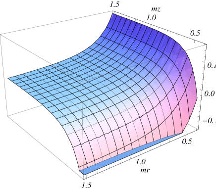
Figure 1: Renormalized FC, $\langle\bar{\psi}\psi\rangle_{\mathrm{ren}}/m^{3}$, in the geometry of a flat boundary in cosmic string spacetime with $q=3$ as a function of the distances from the boundary and from the string.

4 Energy-momentum tensor

In this section we consider another important characteristic of the fermionic vacuum, the VEV of the energy-momentum tensor. This VEV can be evaluated by using the mode sum formula

$$\left\langle 0\left|T_{\mu\nu}\right|0\right\rangle=\frac{i}{2}\sum_{\sigma}[\bar{\psi}_{\sigma}^{(-)}\gamma_{(\mu}\nabla_{\nu)}\psi_{\sigma}^{(-)}-(\nabla_{(\mu}\bar{\psi}_{\sigma}^{(-)})\gamma_{\nu)}\psi_{\sigma}^{(-)}]\ ,$$ (4.1)

where the brackets enclosing the indices mean the simmetrization. Inserting the expression for the negative-energy mode functions, similar to the case of the FC, the VEV is presented in the decomposed form:

$$\left\langle 0\left|T_{\mu\nu}\right|0\right\rangle=\left\langle 0\left|T_{\mu\nu}\right|0\right\rangle_{\mathrm{s}}+\left\langle T_{\mu\nu}\right\rangle_{\mathrm{b}},$$ (4.2)

where the first and second terms on the right-hand side correspond to the boundary-free and boundary-induced parts, respectively. It can be seen that both parts are diagonal. The latter property is not a consequence of the problem geometry. As it has been shown in [43], for a scalar field obeying Dirichlet and Neumann boundary conditions on a plate at $z=0$, the off-diagonal component $\left\langle 0\left|T_{13}\right|0\right\rangle$ does not vanish for a general curvature coupling parameter $\xi$. Only in the special case with $\xi=1/4$ the VEV of the energy-momentum tensor is diagonal.

4.1 Boundary-free part

For the VEV in the boundary-free cosmic string geometry we find the expression (no summation over $\nu$)

$$\left\langle 0\left|T_{\nu}^{\nu}\right|0\right\rangle_{\mathrm{s}}=\frac{q}{\pi^{2}}\sum_{j}\int_{0}^{\infty}dk\,\int_{0}^{\infty}d\lambda\frac{\lambda^{3}}{\omega}g_{\beta}^{(\nu)}(\lambda r),$$ (4.3)

with the notations

$$g_{\beta}^{(0)}(y) = \frac{\omega^{2}}{k^{2}}g_{\beta}^{(3)}(y)=-\frac{\omega^{2}}{\lambda^{2}}[J_{\beta}^{2}(y)+J_{\beta+1}^{2}(y)],$$

$$g_{\beta}^{(1)}(y) = J_{\beta}^{2}(y)+J_{\beta+1}^{2}(y)-\frac{2qj}{y}J_{\beta}(y)J_{\beta+1}(y),$$ (4.4)

$$g_{\beta}^{(2)}(y) = \frac{2qj}{y}J_{\beta}(y)J_{\beta+1}(y).$$

For $r\neq 0$ the renormalization of the boundary-free part is reduced to the subtraction of the corresponding VEV in Minkowski spacetime:

$$\left\langle T_{\mu}^{\nu}\right\rangle_{\mathrm{s,ren}}=\left\langle 0\left|T_{\mu}^{\nu}\right|0\right\rangle_{\mathrm{s}}-\left\langle 0\left|T_{\mu}^{\nu}\right|0\right\rangle_{\mathrm{M}}.$$ (4.5)

In Appendix A we show that the renormalized boundary-free VEV is presented in the form (no summation over $\nu$)

$$\left\langle T_{\nu}^{\nu}\right\rangle_{\mathrm{s,ren}} = \frac{2m^{4}}{\pi^{2}}\bigg{[}\sum_{l=1}^{p}(-1)^{l}\cos\left(\pi l/q\right)F_{\nu}^{(0)}(2mr\sin(\pi l/q))$$ (4.6)

$$+\frac{2q}{\pi}\cos\left(q\pi/2\right)\int_{0}^{\infty}dx\frac{\sinh\left(qx\right)\sinh(x)F_{\nu}^{(0)}(2mr\cosh x)}{\cosh(2qx)-\cos(q\pi)}\bigg{]},$$

where we have defined

$$F_{0}^{(0)}(y) = F_{1}^{(0)}(y)=F_{3}^{(0)}(y)=f_{2}(y),$$

$$F_{2}^{(0)}(y) = -3f_{2}(y)-f_{1}(y),$$ (4.7)

with the notation (3.14). For $q<2$ the first term in the square brackets is absent and the formula (4.6) is reduced to the one derived in [29]. For general case of $q$ an alternative integral representation is given in [38]. For a massless field the corresponding renormalized VEV for the energy-momentum tensor was found in [8, 10]:

$$\left\langle T_{\mu}^{\nu}\right\rangle_{\mathrm{s,ren}}=-\frac{(q^{2}-1)(7q^{2}+17)}{2880\pi^{2}r^{4}}\mathrm{diag}(1,1,-3,1).$$ (4.8)

Fermionic propagators for a massive field are considered in Refs. [22, 23, 29]. Note that in the boundary-free cosmic string spacetime one has the relation $\left\langle T_{0}^{0}\right\rangle_{\mathrm{s,ren}}=\left\langle T_{3}^{3}\right\rangle_{\mathrm{s,ren}}$ for a massive field. The latter is a consequence of the boost invariance along the axis of the cosmic string.

For a massive field and for points near the string, $mr\ll 1$, the leading term in the corresponding asymptotic expansion is given by (4.8) and the renormalized VEV diverges on the string as $r^{-4}$. At large distances, $mr\gg 1$, for $q<2$ the first term in the square brackets in (4.6) is absent and the dominant contribution in the second term comes from the region near the lower limit of the integration. In this case $\left\langle T_{\mu}^{\nu}\right\rangle_{\mathrm{s,ren}}$ is suppressed by the factor $e^{-2mr}$. For $q>2$ the dominant contribution at large distances comes from the $l=1$ term in (4.6) and the suppression factor is $e^{-2mr\sin(\pi/q)}$. Note that the contribution of the first term in the square brackets of (4.6) is always negative for $\nu=0,1,3$, and positive for $\nu=2$. The contribution from the second term has opposite sign for $3+4n<q<5+4n$ with $n=0,1,2,\ldots$. However, for large $q$ this contribution is small.

In figure 2 we plotted the boundary-free parts in the energy density (full curves) and the azimuthal stress (dashed curves) as functions of the distance from the string in units of the Compton wavelength. The numbers near the curves correspond to the values of the parameter $q$. Note that the quantity (no summation over $\nu$) $-\left\langle T_{\nu}^{\nu}\right\rangle_{\mathrm{s,ren}}$, with $\nu=1,2,3$, is the vacuum effective pressure along the corresponding direction. Hence, in the boundary-free cosmic string spacetime the vacuum azimuthal pressure is negative, whereas pressures along the radial and axial directions are positive.

Figure 2: Boundary-free parts in the energy density (full curves) and the azimuthal stress (dashed curves) as functions of the distance from the string for separate values of the parameter $q$ (numbers near the curves).

4.2 Boundary-induced part

For the boundary-induced part of the vacuum energy-momentum tensor we have (no summation over $\nu=0,1,2$)

$$\left\langle T_{\nu}^{\nu}\right\rangle_{\mathrm{b}}=-\frac{q}{\pi^{2}}m\left(m+\partial_{2z}\right)\sum_{j}\int_{0}^{\infty}d\lambda\int_{0}^{\infty}dk\frac{\lambda^{3}}{\omega}g_{\beta}^{(\nu)}(\lambda r)\frac{\cos(2kz)}{k^{2}+m^{2}},$$ (4.9)

with the functions $g_{\beta}^{(\nu)}(y)$ defined in (4.4), and the corresponding axial stress vanishes:

$$\left\langle T_{3}^{3}\right\rangle_{\mathrm{b}}=0.$$ (4.10)

For a massless field the boundary-induced part in the VEV of the energy-momentum tensor vanishes. Note that the latter is not the case for a massless scalar field (see [43]). It can be explicitly checked that the VEV (4.9) obeys the covariant conservation equation $\nabla_{\nu}\langle T_{\mu}^{\nu}\rangle_{\mathrm{b}}=0$, which for the problem under consideration is reduced to the single equation

$$\partial_{r}(r\left\langle T_{1}^{1}\right\rangle_{\mathrm{b}})=\left\langle T_{2}^{2}\right\rangle_{\mathrm{b}}.$$ (4.11)

We have also the trace relation

$$\left\langle T_{\nu}^{\nu}\right\rangle_{\mathrm{b}}=m\langle\bar{\psi}\psi\rangle_{\mathrm{b}}.$$ (4.12)

Further transformations for the components of the boundary-induced part in the VEV of the energy-momentum tensor are given in Appendix A. They are presented in the form (no summation over $\nu$)

$$\left\langle T_{\nu}^{\nu}\right\rangle_{\mathrm{b}} = \frac{2m^{4}}{\pi^{2}}\bigg{[}\sideset{}{{}^{\prime}}{\sum}_{l=0}^{p}(-1)^{l}\cos\left(\pi l/q\right)F_{\nu}(2mz,2mr\sin(\pi l/q))$$ (4.13)

$$+\frac{2q}{\pi}\cos\left(q\pi/2\right)\int_{0}^{\infty}dx\frac{\sinh\left(qx\right)\sinh\left(x\right)}{\cosh(2qx)-\cos(q\pi)}F_{\nu}(2mz,2mr\cosh x)\bigg{]},$$

where

$$F_{0}(x,y) = F_{1}(x,y)=-G_{2}(x,y),$$

$$F_{2}(x,y) = 2G_{2}(x,y)+F(x,y),$$ (4.14)

$$\;F_{3}(x,y) = 0.$$

In (4.13), the function $G_{\nu}(x,y)$ is defined as

$$G_{\nu}(x,y)=e^{x}\int_{x}^{\infty}du\,e^{-u}f_{\nu}(\sqrt{u^{2}+y^{2}}),$$ (4.15)

and the function $F(x,y)$ is given by (3.23). As we see, the boundary-induced part in the energy density is equal to the radial stress: $\left\langle T_{0}^{0}\right\rangle_{\mathrm{b}}=\left\langle T_{1}^{1}\right\rangle_{\mathrm{b}}$ and the axial stress vanishes. By using the relation (A.7) we can see that $\partial_{y}[yF_{1}(x,y)]=$ $F_{2}(x,y)$. With this relation the covariant conservation equation (4.11) is explicitly checked.

Alternative expressions for the boundary-induced parts in the energy density and in the azimuthal stress are given by formulas (A.4) and (A.13) in Appendix A. In particular, from (A.4) it follows that the boundary-induced part in the energy density is always negative for $r>0$. For the investigation of the boundary-induced VEV near the cosmic string it is more convenient to use the representations (A.4) and (A.13). The leading contributions come from the terms with $j=1/2$ in the series for $\mathcal{I}(q,y)$. To the leading order one gets

$$\left\langle T_{\mu}^{\nu}\right\rangle_{\mathrm{b}}\approx\frac{qm^{q+3}r^{q-1}}{2^{(q-1)/2}\pi^{2}}\frac{f_{(q+1)/2}(2mz)-2mzf_{(q+3)/2}(2mz)}{\left(q+2\right)\Gamma((q+1)/2)}\mathrm{diag}(1,1,q,0),$$ (4.16)

and the boundary-induced part vanishes on the string for $q>1$ and $z\neq 0$. Note that from the relation (A.8) in Appendix A it follows that the function in the numerator of (4.16) is negative.

For $q=1$ there is only contribution from the term with $l=0$ and from (4.13) we obtain the result for a plate in Minkowski spacetime (note that in this case the asymptotic expression (4.16) is exact):

$$\left\langle T_{\mu}^{\nu}\right\rangle_{\mathrm{b}}^{\mathrm{(M)}}=\frac{m^{4}}{3\pi^{2}}[f_{1}(2mz)-2mzf_{2}(2mz)]\,\mathrm{diag}(1,1,1,0).$$ (4.17)

In this case the vacuum stresses along the directions parallel to the plate are equal to the the energy density. This result is a consequence of the Lorentz invariance of the problem along these directions. Note that in the presence of the cosmic string this invariance is broken. However, the radial stress remains equal to the energy density. Formula (4.17) is a special case of a more general result given in [52] for a plate in flat spacetime with toroidally compactified spatial dimensions.

Extracting the term $l=0$ in (4.13), the boundary-induced part in the VEV of the energy-momentum tensor can be written in the form

$$\left\langle T_{\mu}^{\nu}\right\rangle_{\mathrm{b}}=\left\langle T_{\mu}^{\nu}\right\rangle_{\mathrm{b}}^{\mathrm{(M)}}+\left\langle T_{\mu}^{\nu}\right\rangle_{\mathrm{b}}^{\mathrm{(s)}},$$ (4.18)

where $\left\langle T_{\mu}^{\nu}\right\rangle_{\mathrm{b}}^{\mathrm{(s)}}$ comes from the nontrivial topology of the cosmic string spacetime. We can see that the latter is finite everywhere except at the point $r=z=0$. The divergences on the boundary are contained in the Minkowskian part. Near the boundary, for $z\ll r$, to the leading order one has (no summation over $\nu=0,1,2$):

$$\left\langle T_{\nu}^{\nu}\right\rangle_{\mathrm{b}}\approx\left\langle T_{\nu}^{\nu}\right\rangle_{\mathrm{b}}^{\mathrm{(M)}}\approx-\frac{m}{12\pi^{2}z^{3}}.$$ (4.19)

For points away from the boundary the renormalized VEV of the energy-momentum tensor is presented as

$$\left\langle T_{\mu}^{\nu}\right\rangle_{\mathrm{ren}}=\left\langle T_{\mu}^{\nu}\right\rangle_{\mathrm{s,ren}}+\left\langle T_{\mu}^{\nu}\right\rangle_{\mathrm{b}},$$ (4.20)

where the boundary-free and boundary-induced parts are given by (4.6) and (4.13), respectively. The dependence of the corresponding energy density (left plot) and the azimuthal stress (right plot) on the distances from the string and from the boundary is presented in figure 3 for the geometry of cosmic string with $q=3$. In the case of the energy density both the boundary-free and boundary-induced parts are negative. For the azimuthal stress, the boundary-free part is positive whereas the boundary-induced part is negative. The latter dominates for points near the boundary.

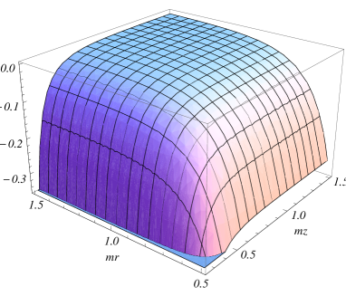
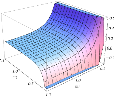
Figure 3: VEV of the the energy density, $m^{-4}\langle T_{0}^{0}\rangle_{\mathrm{ren}}$ (left plot), and the azimuthal stress, $m^{-4}\langle T_{2}^{2}\rangle_{\mathrm{ren}}$ (right plot), as functions of the distances from the string and from the boundary for $q=3$.

5 Conclusion

In this paper we have considered the interplay of topological and boundary-induced quantum effects in the fermionic vacuum. The nontrivial topology of the background spacetime is due to the presence of an idealized cosmic string and the fermionic field obeys MIT bag boundary condition on a plane perpendicular to the string. As physical characteristics of the vacuum state, we have investigated the FC and the VEV of the energy-momentum tensor. For the evaluation of these VEVs a complete set of mode functions for the corresponding boundary value problem is necessary. A crucial point in this paper was the obtainment of both positive- and negative-energy wave functions in section 2. These functions are given by the expressions (2.29) and (2.43), respectively. They can be used for the investigation of various quantum electrodynamics processes around the cosmic string in the presence of boundary involving electrons and positrons.

The FC is decomposed into the boundary-free and boundary-induced contributions. The renormalized boundary-free part is given by (3.13) and, for a general value of $q$, it vanishes for a massless field. As to the boundary-induced part, it is finite for points outside of boundary and is given by the formula (3.22). An alternative representation is provided by (3.16). The expression for the boundary-induced part in FC is simplified for the case of a massless field, Eq. (3.17). In this case the boundary-free part vanishes and the boundary-induced part is negative for points outside the string. For points near the string the boundary-induced part in FC behaves as $r^{q-1}$. The latter is the case for a massive field also. On the boundary the FC is divergent. For points near the boundary the part $\langle\bar{\psi}\psi\rangle_{\mathrm{b}}^{\mathrm{(M)}}$ dominates and the FC is negative. The remained part in $\langle\bar{\psi}\psi\rangle_{\mathrm{b}}$ corresponds to the contribution induced by the nontrivial topology of the string and for $r\neq 0$ it is finite on the boundary. At large distance from the boundary and for a massless field the leading term in the boundary-induced FC is given by (3.21). Compared with the case of the Minkowski bulk, the presence of the cosmic string leads to an additional suppression in the form of the factor $(r/2z)^{q-1}$. For a massive field and at large distances from the boundary, the boundary-induced part of FC is exponentially suppressed.

Another calculation developed in this paper is the VEV of the energy-momentum tensor. Similar to the case of FC we have the decomposition (4.2). In this way, for points away from the boundary, the renormalization is reduced to the one for the boundary-free part. For the general case of the parameter $q$, the renormalized value for the latter is given by (4.6). This formula generalizes various special cases, previously discussed in the literature. For points near the string the pure string part diverges as $r^{-4}$. In the opposite limit, at distances larger than the Compton wavelength for a fermionic particle, $\left\langle T_{\mu}^{\nu}\right\rangle_{\mathrm{s,ren}}$ is suppressed by the factor $e^{-2mr}$ for $q<2$ and by the factor $e^{-2mr\sin(\pi/q)}$ for $q>2$.

The boundary-induced part in the VEV of the energy-momentum tensor, $\left\langle T_{\mu}^{\nu}\right\rangle_{\mathrm{b}}$, is given by the expression (4.13). This part is diagonal and vanishes for a massless field. Note that for a scalar field with general curvature coupling parameter the part in the VEV of the energy-momentum tensor induced by Dirichlet and Neumann boundaries perpendicular to the plate has nonzero off-diagonal component $\left\langle T_{3}^{1}\right\rangle_{\mathrm{b}}$ (see [43]). The latter is zero in the special case of the curvature coupling parameter $\xi=1/4$. Another difference, compared with the fermionic case, is that for a massless scalar field the boundary-induced part does not vanish. For a massive fermionic field the boundary-induced part in the radial stress is equal to the energy density and the axial stress vanishes. For $q>1$ and $z\neq 0$, the boundary-induced part vanishes on the string with the asymptotic behavior given by (4.16). Near the boundary the VEV is dominated by the part corresponding to a plate in Minkowski spacetime. The latter is given by the expression (4.17). The corresponding radial and azimuthal stresses are equal to the energy density and the latter is negative. For points near the string, the boundary-free part in the vacuum energy-momentum tensor dominates. The corresponding energy density is negative, whereas the azimuthal stress is positive.

Appendix A Evaluation of the energy density and azimuthal stress

In this appendix we give some details related with the transformation of the expressions for the boundary-induced parts in the VEVs of the energy density and the azimuthal stress. First we consider the energy density. Our starting point is the expression (4.9) with $g_{\beta}^{(0)}(\lambda,\lambda r)$ defined in (4.4). As the first step we insert the representation

$$\omega=-\frac{2}{\sqrt{\pi}}\int_{0}^{\infty}ds\,\partial_{s^{2}}e^{-\left(k^{2}+\lambda^{2}+m^{2}\right)s^{2}}.$$ (A.1)

Changing the order of integrations in (4.9), the integral over $\lambda$ is expressed in terms of the modified Bessel function of the first kind. After the integration by parts in the integral over $s$, we find the expression

$$\left\langle T_{0}^{0}\right\rangle_{\mathrm{b}} = -\frac{qm}{\sqrt{2\pi}\pi^{2}r^{3}}\left(m+\partial_{2z}\right)\int_{0}^{\infty}dy\,\sqrt{y}e^{-y}$$ (A.2)

$$\times\mathcal{I}(q,y)\int_{0}^{\infty}dk\,\frac{\cos(2kz)}{k^{2}+m^{2}}e^{-\left(k^{2}+m^{2}\right)r^{2}/2y},$$

with $\mathcal{I}(q,y)$ defined in (3.11). The presence of the factor $(k^{2}+m^{2})^{-1}$ in the integrand of (A.2) leads to some complication in the further evaluation of the VEV when compared with the case of the FC.

Here we use the relation

$$\left(m+\partial_{x}\right)\frac{\cos(kx)}{k^{2}+m^{2}}=e^{mx}\int_{x}^{\infty}dt\,e^{-mt}\cos(kt).$$ (A.3)

Substituting this into (A.2) we first integrate over $k$ with the result:

$$\left\langle T_{0}^{0}\right\rangle_{\mathrm{b}}=-\frac{qm}{\pi^{2}r^{4}}e^{2mz}\int_{z}^{\infty}dte^{-2mt}\int_{0}^{\infty}dy\,ye^{-m^{2}r^{2}/(2y)-y(2t^{2}/r^{2}+1)}\mathcal{I}(q,y).$$ (A.4)

Now, by using the formula (3.12), the integral over $y$ is given in terms of the Macdonald function and we come to the final expression

$$\left\langle T_{0}^{0}\right\rangle_{\mathrm{b}} = -\frac{2m^{4}}{\pi^{2}}\bigg{[}\sideset{}{{}^{\prime}}{\sum}_{l=0}^{p}(-1)^{l}\cos\left(\pi l/q\right)G_{2}(2mz,2mr\sin(\pi l/q))$$ (A.5)

$$+\frac{2q}{\pi}\cos\left(q\pi/2\right)\int_{0}^{\infty}dx\frac{\sinh\left(qx\right)\sinh\left(x\right)}{\cosh(2qx)-\cos(q\pi)}G_{2}(2mz,2mr\cosh x)\bigg{]},$$

where the function $G_{\nu}(x,y)$ is defined by (4.15). By using the relations

$$\partial_{x}f_{\nu}(x) = -xf_{\nu+1}(x),$$

$$x\partial_{x}f_{\nu}(x) = -f_{\nu-1}(x)-2\nu f_{\nu}(x),$$ (A.6)

for this function $G_{\nu}(x,y)$ we get the following formula

$$y^{2}G_{\nu+1}(x,y)=\left(2\nu-1\right)G_{\nu}(x,y)+f_{\nu-1}(\sqrt{x^{2}+y^{2}})-xf_{\nu}(\sqrt{x^{2}+y^{2}}).$$ (A.7)

In particular, $G_{\nu}(x,0)$ is expressed in terms of the Macdonald function (see also [51]):

$$G_{\nu}(x,0)=\frac{xf_{\nu}(x)-f_{\nu-1}(x)}{2\nu-1}.$$ (A.8)

Now we turn to the azimuthal stress. The corresponding expression from (4.9), with $g_{\beta}^{(2)}(\lambda,y)$ defined in (4.4), can be written in the form

$$\left\langle T_{22}\right\rangle_{\mathrm{b}} = 2m\frac{q^{2}}{\pi^{2}}\left(m+\partial_{2z}\right)\sum_{j}j\left(2qj-1-r\partial_{r}\right)$$ (A.9)

$$\times\int_{0}^{\infty}dk\,\frac{\cos(2kz)}{k^{2}+m^{2}}\int_{0}^{\infty}d\lambda\frac{\lambda}{\omega}J_{qj-1/2}^{2}(\lambda r).$$

By using the representation (3.9) we evaluate the integral over $\lambda$ in terms of the modified Bessel function. Making use of the relations

$$(qj-1/2-y\partial_{y})e^{-y}I_{qj-1/2}(y)=ye^{-y}[I_{qj-1/2}(y)-I_{qj+1/2}(y)],$$ (A.10)

and

$$qj[I_{qj-1/2}(y)-I_{qj+1/2}(y)]=(y\partial_{y}-y+1/2)[I_{qj-1/2}(y)+I_{qj+1/2}(y)],$$ (A.11)

we arrive to the expression

$$\left\langle T_{2}^{2}\right\rangle_{\mathrm{b}} = -\frac{4mq}{\pi^{5/2}}\int_{0}^{\infty}ds\,y^{2}e^{-y}(y\partial_{y}-y+1/2)\mathcal{I}(q,y)$$ (A.12)

$$\times\int_{0}^{\infty}dk\,\left(m+\partial_{2z}\right)\frac{\cos(2kz)}{k^{2}+m^{2}}e^{-(k^{2}+m^{2})s^{2}},$$

where $y=r^{2}/(2s^{2})$. The $k$-integration is explicitly done by using the representation (A.3) with the result

$$\left\langle T_{2}^{2}\right\rangle_{\mathrm{b}} = -2\frac{qm}{\pi^{2}}e^{2mz}\int_{z}^{\infty}dte^{-2mt}\int_{0}^{\infty}dy\,y$$ (A.13)

$$\times e^{-m^{2}r^{2}/2y-y(2t^{2}/r^{2}+1)}\left(y\partial_{y}-y+1/2\right)\mathcal{I}(q,y).$$

Now we employ the formula (3.12). After the integration over $y$ we find the expression

$$\left\langle T_{2}^{2}\right\rangle_{\mathrm{b}} = \frac{2m^{4}}{\pi^{2}}\bigg{[}\sideset{}{{}^{\prime}}{\sum}_{l=0}^{p}(-1)^{l}\cos\left(\pi l/q\right)F_{2}(2mz,2mr\sin\left(\pi l/q\right))$$ (A.14)

$$+\frac{2q}{\pi}\cos\left(q\pi/2\right)\int_{0}^{\infty}dx\frac{\sinh\left(qx\right)\sinh x}{\cosh(2qx)-\cos(q\pi)}F_{2}(2mz,2mr\cosh x)\bigg{]},$$

with the notation

$$F_{2}(x,y)=y^{2}G_{3}(x,y)-G_{2}(x,y).$$ (A.15)

An alternative expression (4.14) for the function $F_{2}(x,y)$ is obtained by using the relation (A.7).

Having the energy density and the azimuthal stress we can find the radial stress with the help of the trace relation (4.12). By using the expression (3.22) for the FC, we can see that the boundary-induced part in the radial stress is equal to the energy density.

Note that the transformations described above can also be done for the boundary-free parts in the energy density and the azimuthal stress. By using (3.9) we find

$$\left\langle 0|T_{0}^{0}|0\right\rangle_{\mathrm{s}} = \frac{q}{2\pi^{2}r^{4}}\int_{0}^{\infty}dy\,ye^{-m^{2}r^{2}/2y-y}\mathcal{I}(q,y),$$

$$\left\langle 0|T_{2}^{2}|0\right\rangle_{\mathrm{s}} = \frac{q}{\pi^{2}r^{4}}\int_{0}^{\infty}dy\,ye^{-m^{2}r^{2}/2y-y}\,(y\partial_{y}-y+1/2)\mathcal{I}(q,y).$$ (A.16)

Now substituting (3.12), we see that the contribution of the $l=0$ term corresponds to the VEV in boundary-free Minkowski spacetime. The latter is subtracted in the renormalization procedure and for the renormalized VEVs of the energy density and the azimuthal stress we find the representation (4.6). From the boost invariance along the axis of the cosmic string we have $\left\langle 0|T_{3}^{3}|0\right\rangle_{\mathrm{s,ren}}=\left\langle 0|T_{0}^{0}|0\right\rangle_{\mathrm{s,ren}}$. The radial stress is found from the trace relation $\left\langle 0|T_{\nu}^{\nu}|0\right\rangle_{\mathrm{s,ren}}=m\langle\bar{\psi}\psi\rangle_{\mathrm{s,ren}}$, by using the expression (3.13) for the FC.

References

• [1] E. Elizalde, S.D. Odintsov, A. Romeo, A.A. Bytsenko and S. Zerbini, Zeta Regularization Techniques with Applications (World Scientific, Singapore, 1994); V.M. Mostepanenko and N.N. Trunov, The Casimir Effect and Its Applications (Clarendon, Oxford, 1997); K.A. Milton, The Casimir Effect: Physical Manifestation of Zero-Point Energy (World Scientific, Singapore, 2002); M. Bordag, G.L. Klimchitskaya, U. Mohideen, and V.M. Mostepanenko, Advances in the Casimir Effect (Oxford University Press, Oxford, 2009); Lecture Notes in Physics: Casimir Physics, Vol. 834, edited by D. Dalvit, P. Milonni, D. Roberts, and F. da Rosa (Springer, Berlin, 2011).
• [2] A. Vilenkin and E.P.S. Shellard, Cosmic Strings and Other Topological Defects (Cambridge University Press, Cambridge, England, 1994).
• [3] S. Sarangi and S.H.H. Tye, Phys. Lett. B 536, 185 (2002); E.J. Copeland, R.C. Myers, and J. Polchinski, JHEP 06, 013 (2004); G. Dvali and A. Vilenkin, JCAP 0403, 010 (2004).
• [4] E.J. Copeland, L. Pogosian, and T. Vachaspati, Class. Quantum Grav. 28, 204009 (2011).
• [5] T.M. Helliwell and D.A. Konkowski, Phys. Rev. D 34, 1918 (1986).
• [6] W.A. Hiscock, Phys. Lett. B 188, 317 (1987).
• [7] B. Linet, Phys. Rev. D 35, 536 (1987).
• [8] V.P. Frolov and E.M. Serebriany, Phys. Rev. D 35, 3779 (1987).
• [9] J.S. Dowker, Phys. Rev. D 36, 3095 (1987).
• [10] J.S. Dowker, Phys. Rev. D 36, 3742 (1987).
• [11] A.G. Smith, in The Formation and Evolution of Cosmic Strings, Proceedings of the Cambridge Workshop, Cambridge, England, 1989, edited by G.W. Gibbons, S.W. Hawking, and T. Vachaspati (Cambridge University Press, Cambridge, England, 1990).
• [12] G.E.A. Matsas, Phys. Rev. D 41, 3846 (1990).
• [13] B. Allen and A.C. Ottewill, Phys. Rev. D 42, 2669 (1990).
• [14] M. Bordag, Ann. Phys. (Leipzig) 47, 93 (1990).
• [15] B. Allen, J.G. Mc Laughlin, and A.C. Ottewill, Phys. Rev. D 45, 4486 (1992).
• [16] T. Souradeep and V. Sahni, Phys. Rev. D 46, 1616 (1992).
• [17] K. Shiraishi and S. Hirenzaki, Class. Quantum Grav. 9, 2277 (1992).
• [18] V.B. Bezerra and E.R. Bezerra de Mello, Class. Quantum Grav. 11, 457 (1994); E.R. Bezerra de Mello, Class. Quantum Grav. 11, 1415 (1994).
• [19] D. Fursaev, Class. Quantum Grav. 11, 1431 (1994).
• [20] G. Cognola, K. Kirsten, and L. Vanzo, Phys. Rev. D 49, 1029 (1994).
• [21] M.E.X. Guimarães and B. Linet, Commun. Math. Phys. 165, 297 (1994).
• [22] B. Linet, J. Math. Phys. (N.Y.) 36, 3694 (1995).
• [23] E.S. Moreira Jnr, Nucl. Phys. B 451, 365 (1995).
• [24] B. Allen, B.S. Kay, and A.C. Ottewill, Phys. Rev. D 53, 6829 (1996).
• [25] M. Bordag, K. Kirsten, and S. Dowker, Commun. Math. Phys. 182, 371 (1996).
• [26] D. Iellici, Class. Quantum Grav. 14, 3287 (1997).
• [27] N.R. Khusnutdinov and M. Bordag, Phys. Rev. D 59, 064017 (1999).
• [28] J. Spinelly and E.R. Bezerra de Mello, Class. Quantum Grav. 20, 873 (2003).
• [29] V.B. Bezerra and N.R. Khusnutdinov, Class. Quantum Grav. 23, 3449 (2006).
• [30] O. Schröder, N. Graham, M. Quandt, and H. Weigel, J. Phys. A 41, 164049 (2008); N. Graham, M. Quandt, and H. Weigel, Phys. Rev. D 84, 025017 (2011).
• [31] Yu.A. Sitenko and N.D. Vlasii, Class. Quantum Grav. 26, 195009 (2009); Yu.A. Sitenko and N.D. Vlasii, Class. Quantum Grav. 29, 095002 (2012).
• [32] P.C.W. Davies and V. Sahni, Class. Quantum Grav. 5, 1 (1988).
• [33] E.R. Bezerra de Mello and A. A. Saharian, JHEP 04 (2009) 046; E.R. Bezerra de Mello and A. A. Saharian, JHEP 08 (2010) 038.
• [34] A.C. Ottewill and P. Taylor, Phys. Rev. D 82, 104013 (2010); A.C. Ottewill and P. Taylor, Class. Quantum Grav. 28, 015007 (2011).
• [35] E.R. Bezerra de Mello and A. A. Saharian, J. Phys. A: Math. Theor. 45, 115402 (2012).
• [36] E.R. Bezerra de Mello, V.B. Bezerra, A.A. Saharian, and A.S. Tarloyan, Phys. Rev. D 74, 025017 (2006).
• [37] V.V. Nesterenko and I.G. Pirozhenko, Class. Quantum Grav. 28, 175020 (2011).
• [38] E.R. Bezerra de Mello, V.B. Bezerra, A.A. Saharian, and A.S. Tarloyan, Phys. Rev. D 78, 105007 (2008).
• [39] E.R. Bezerra de Mello, V.B. Bezerra, A.A. Saharian, and V.M. Bardeghyan, Phys. Rev. D 82, 085033 (2010); S. Bellucci, E.R. Bezerra de Mello, and A.A. Saharian, Phys. Rev. D. 83, 085017 (2011); E.R. Bezerra de Mello, F. Moraes, and A.A. Saharian, Phys. Rev. D 85, 045016 (2012).
• [40] I. Brevik and T. Toverud, Class. Quantum Grav. 12, 1229 (1995).
• [41] E.R. Bezerra de Mello, V.B. Bezerra, and A.A. Saharian, Phys. Lett. B 645, 245 (2007).
• [42] G. Fucci and K. Kirsten, JHEP 03, 016 (2011); G. Fucci and K. Kirsten, J. Phys. A: Math. Theor. 44, 295403 (2011).
• [43] E.R. Bezerra de Mello and A.A. Saharian, Class. Quantum Grav. 28, 145008 (2011).
• [44] E.R. Bezerra de Mello, A.A. Saharian, and A.Kh. Grigoryan, J. Phys. A: Math. Theor. 45, 374011 (2012).
• [45] E.R. Bezerra de Mello and A.A. Saharian, Class. Quantum Grav. 29, 035006 (2012).
• [46] A.A. Saharian and A.S. Kotanjyan, Eur. Phys. J. C 71, 1765 (2011); A.A. Saharian and A.S. Kotanjyan, Phys. Lett. B 713, 133 (2012); E.R. Bezerra de Mello, V.B. Bezerra, H.F. Mota, A.A. Saharian, Phys. Rev. D, in press, arXiv:1205.6914.
• [47] D.R. Nelson, Defects and Geometry in Condensed Matter Physics (Cambridge University Press, Cambridge, 2002); G.E. Volovik, The Universe in a Helium Droplet (Clarendon Press, Oxford, 2003).
• [48] A. Vilenkin, Phys. Rev. D 23, 852 (1981).
• [49] J.R. Gott III, Astrophys. J. 288, 422 (1985); W. Hiscock, Phys. Rev. D 31, 3288 (1985); B. Linet, Gen. Relativ. Gravit. 17, 1109 (1985); D. Garfinkle, Phys. Rev. D 32, 1323 (1985).
• [50] A. Krishnan, et al, Nature 388, 451 (1997); S.N. Naess, A. Elgsaeter, G. Helgesen, and K.D. Knudsen, Sci. Technol. Adv. Mater. 10, 065002 (2009).
• [51] A.P. Prudnikov, Yu.A. Brychkov, and O.I. Marichev, Integrals and Series (Gordon and Breach, New York, 1986), Vol. 2.
• [52] E. Elizalde, S.D. Odintsov, and A.A. Saharian, Phys. Rev. D 83, 105023 (2011).