Multidimensional realistic modelling of Cepheid-like variables. I: Extensions of the ANTARES code.

Abstract

We have extended the ANTARES code to simulate the coupling of pulsation with convection in Cepheid-like variables in an increasingly realistic way, in particular in multidimensions, 2D at this stage. Present days models of radially pulsating stars assume radial symmetry and have the pulsation-convection interaction included via model equations containing ad hoc closures and moreover parameters whose values are barely known. We intend to construct ever more realistic multidimensional models of Cepheids. In the present paper, the first of a series, we describe the basic numerical approach and how it is motivated by physical properties of these objects which are sometimes more, sometimes less obvious. – For the construction of appropriate models a polar grid co-moving with the mean radial velocity has been introduced to optimize radial resolution throughout the different pulsation phases. The grid is radially stretched to account for the change of spatial scales due to vertical stratification and a new grid refinement scheme is introduced to resolve the upper, hydrogen ionisation zone where the gradient of temperature is steepest. We demonstrate that the simulations are not conservative when the original weighted essentially non-oscillatory method implemented in ANTARES is used and derive a new scheme which allows a conservative time evolution. The numerical approximation of diffusion follows the same principles. Moreover, the radiative transfer solver has been modified to improve the efficiency of calculations on parallel computers. We show that with these improvements the ANTARES code can be used for realistic simulations of the convection-pulsation interaction in Cepheids. We discuss the properties of several numerical models of this kind which include the upper 42% of a Cepheid along its radial coordinate and assume different opening angles. The models are suitable for an in-depth study of convection and pulsation in these objects.

1 Introduction

The series of papers introduced by this article deals with the construction and analysis of time-dependent, nonlinear numerical models for classical, radially pulsating variable stars (Cepheids, RR Lyr,…) in multiple dimensions. The models are set up to investigate the pulsation-convection interaction and, eventually, nonradial pulsations in such stars. In the present paper we describe the extension of the ANTARES code (Muthsam et al., 2010) necessary for such an investigation. We additionally discuss effects of resolution and other issues. A subsequent paper (Muthsam et al., 2012), paper II, will deal with an investigation of the physical results.

The following considerations have motivated this work. One of the early successes of numerical modelling of the dynamics of astrophysical objects were simulations of Cepheid (or RR Lyr, W Vir,…) pulsations. It was one of the few time-dependent nonlinear problems in astrophysics where the approximation of perfect spherical symmetry was sufficiently good while at the same time observations at the dynamical timescale were readily available. Even decades earlier systematic trends of the shapes of the lightcurve with period, the famous Hertzsprung progression in classical Cepheids, had been established (Hertzsprung 1926). Interest in the subject continued to be kindled by the importance of these variable stars for the understanding of stellar evolution, in particular when discrepancies between masses derived from stellar evolution considerations and from pulsation properties were found (Cox 1980 and Keller 2008). The decisive role of Cepheids in gauging the cosmic distance scale is well known (see the extensive discussion in de Grijs 2011, e.g.) and the precise calibration of relations between mass, luminosity, and metallicity for different types of classical variables is of general astrophysical interest.

Linear stability considerations suggested the excitations of the pulsations through the ionisation of hydrogen and, in particular, helium (Zhevakin 1953, Cox 1960, Baker & Kippenhahn 1962). The first nonlinear, time-dependent calculations soon followed. For pioneering nonlinear work see Christy (1962), Aleshin (1964), Christy (1964), and Cox et al. (1966).

Spherical symmetry allowed the problem to be treated computationally in one spatial dimension and made it accessible to the computing resources of that period. The subsequent decades, essentially till now, have witnessed substantial refinements of computational methods and input physics. Let us mention the inclusion of radiative transfer for the outer zones instead of the diffusion approximation, better numerics including adaptive grids, more realistic opacities and the like. There now exists a considerable number of codes of that kind with various properties such as described in Fokin (1990), Dorfi & Feuchtinger (1991), Bono & Stellingwerf (1994), Buchler et al. (1997) and Smolec & Moskalik (2008).

It soon became apparent that in order to properly represent important observational facts such as the red edge of the Cepheid instability strip convection had to be included and that attempts to accomplish this by incorporating standard mixing length theory into a pulsation code failed (Tuggle & Iben, 1973). Consequently, practically all groups working on the nonlinear hydrodynamics of pulsating stars included convection models which from the outset were meant to apply to a changing environment, essentially extensions of the mixing length approach or models for the time evolution of the turbulent kinetic energy (TKE).

While this improved matters in many respects, it certainly did not solve the problem of constructing an accurate, predictive model of the convection-pulsation interaction in these stars. Since such models cannot be derived from basic principles alone, a variety of recipes for modelling the convective flux is in use (and is discussed in the next paper of this series). The same holds for many other physical quantities appearing in these models. Many closure constants, up to eight, “the $\alpha\mbox{'s}$”, are needed to fully specify the model equations currently used for the one-dimensional calculations (see the impressive compilation in Buchler & Kolláth 2000). Their values are unknown and must be determined somehow. Common ways to do so include adjusting the parameters to match some observable quantities or simply guessing them. Consequently, even if observed properties are reproduced, the extent to which this success can be justifiably ascribed to the model and does not constitute a mere result of the fitting procedure remains doubtful. It most likely lacks the deeper physical correctness intended to achieve with unknown consequences for further interpretations based on such a model.

The state of knowledge has recently been discussed in the review by Buchler (2009). There, he addresses the use of time dependent mixing length theory as the “dominant deficiency” in Cepheid modelling (see also Buchler (1997)). Again in a review, Marconi (2009) emphasized the proper inclusion of convection for modelling RR Lyr stars.

Recently, activities have commenced to address this issue. Gastine & Dintrans (2011) thoroughly analyse physically simplified 2D models to elucidate basic mechanisms of the pulsation-convection interaction (see also literature cited therein). Geroux & Deupree (2011) have reassumed very early work by Deupree (1980). Their calculations are in 3D, albeit with quite low resolution at present. Various physical simplifications have been made in this work (no realistic microphysics, adiabatic stratification), but more realistic microphysics, opacities, and an energy equation based on the diffusion approximation are intended to be included in future investigations.

This is the context in which we present the extension of the ANTARES code for the type of research at hand. We extend the main features of the code (radiation-hydrodynamics with radiative transfer equations in the outer regions, realistic microphysics and opacities, high-resolution numerics, optional grid-refinement) as required for work on nonlinear stellar pulsation. We furthermore add a moving grid (moving at the upper boundary with the mean vertical surface velocity). While the main part of ANTARES is designed for the 1D, 2D, and 3D case, for our present work only the 1D and 2D case have been implemented. This is due to the fact that the extremely steep gradients near the hydrogen ionisation zone make even an adequately resolved 2D calculation a computationally very expensive enterprise. Undoubtedly, however, in the future we will also include the option of performing numerical simulations of this kind in 3D.

At first sight it may look astonishing that we are going to undertake 2D calculations for the time being. After all, meaningful 3D models of solar granulation exist since decades (Nordlund, 1982). For Cepheids, however, the circumstances are different. We find a few remarks on the 2D model atmospheres of Cepheids in Freytag et al. (2012). The difficulties are basically the same as those encountered in the simulation of A-type stars and extensively discussed for them by Kupka, Ballot, & Muthsam (2009) and, for Cepheids, in Sect. 3 of the present article where also a few remarks on computational demands are provided. – The 3D nature of the simulations presented in Geroux & Deupree (2011) does not contradict those remarks, since their work considers an adiabatic test case whose idealised microphysics lacks the properties which ultimately lead to the aforementioned problems.

With the goal of modelling such stars in multidimensions with an ever increasing degree of realism we have extended the ANTARES code and continue to do so, maintaining its basic design principles and ingredients as described in Muthsam et al. (2010), namely

• high resolution numerics of the ENO variety

• realistic equation of state and microphysics

• radiative transfer in the diffusion approximation or using the static radiative transfer equations

• parallelization based on MPI and OpenMP.

For our present specific purpose extensions are necessary which are either obvious from the outset or which experience has taught to be indispensable, namely

• the use of polar coordinates

• a moving grid to follow the pulsations of the star

• a radially stretched grid for coping with the vast differences in length scales between the stellar surface and the interior

• adaption of the treatment of hydrodynamics and radiative transfer to these changed paradigms

• specific forms of grid refinement to properly cope with the fast spatial variation of quantities in very localized regions

• considerations of how to formulate the numerical scheme given the requirements of the objects envisaged for research.

The aim of the paper is, therefore,

• to discuss just those numerical considerations and how they are brought about by the physics of pulsating stars

• and to provide an overview of what is accessible to multidimensional numerical modelling of Cepheids and related variables presently or in the foreseeable future.

For that purpose we have organised the remaining sections as follows. We first present the equations of radiative hydrodynamics on a stretched, co-moving and polar grid and some numerical methods adapted to this setting. In Sect. 3 we provide the parameters of our model and investigate the restrictions resulting from the steep gradient in the H-ionisation zone, while in Sect. 4 we analyse the effects of resolution. Finally, we discuss the usefulness of the calculated simulations, their strength and weaknesses, and possible improvements in Sect. 5 before we provide our conclusions in Sect. 6.

model	aperture	grid points		stretching	subgrid	grid	radial	refined radial
nr.	angle	radial	polar	factor	modelling	refinement	cell size	cell size
1	10o	510	800	1.011	no	no	0.47 …124 Mm
2	3o	510	300	1.011	yes	no	0.47 …124 Mm
3	3o	510	300	1.011	yes	yes	0.47 …124 Mm	0.32 …0.80 Mm
4	1o	800	300	1.007	yes	no	0.29 …79 Mm

Table 1:  Grid parameters for the different numerical Cepheid models discussed in this paper.

2 Numerical methods

The simulations of radially pulsating stars are performed on a stretched, polar, and moving grid. We first introduce the basic conservation laws governing the time evolution of our numerical models in Sect. 2.1 and define subsequently the computational grid (Sect. 2.2). In Sect. 2.3 the necessary alterations for the radiative transfer equation (RTE) are explained in detail. They are not only required for realistic simulations of layers near the stellar surface, but also alleviate the restrictions on time stepping (see Sect. 3.2). In Sect. 2.4 a new set of ENO-coefficients is presented that ensures conservation of the hydrodynamic quantities on a stretched polar grid. Similar adaptations for discretising diffusive fluxes are discussed in Sect. 2.5 while Sect. 2.6 explains our optional subgrid scale modelling. Finally, Sect. 2.7 explains the setup of initial and boundary conditions of the simulations.

2.1 Conservation equations

Including the grid velocity $\overrightarrow{u_{g}}$ in the conservation equations for mass, momentum, and total (kinetic plus thermal) energy we obtain as our set of dynamical equations

$$\frac{\partial\rho}{\partial t}=-\nabla\cdot\left[\vec{I}-\rho\overrightarrow{u_{g}}\right],$$ (1)

$$\frac{\partial\vec{I}}{\partial t}=-\nabla\cdot\left[\frac{\vec{I}\vec{I}}{\rho}-\vec{I}\overrightarrow{u_{g}}-\overline{\sigma}+p\cdot\mbox{Id}\right]+\frac{source}{r}+\rho\vec{g},$$ (2)

$$\frac{\partial e}{\partial t}=-\nabla\cdot\left[\frac{\vec{I}}{\rho}\left(e+p\right)-e\overrightarrow{u_{g}}-\frac{\vec{I}}{\rho}\cdot\overline{\sigma}\right]+\vec{g}\cdot\vec{I}+Q_{\rm rad},$$ (3)

where the term containing

$$source=\left(\begin{array}[]{r}2p+\frac{I_{\varphi}^{2}+I_{\theta}^{2}}{\rho}\\ \frac{-I_{r}I_{\varphi}+I_{\varphi}I_{\theta}\cot\theta}{\rho}\\ -p\cot\theta-\frac{I_{r}I_{\theta}+I_{\varphi}^{2}\cot\theta}{\rho}\end{array}\right)$$ (4)

originates from introducing spherical coordinates. $\overline{\sigma}$ is the viscous stress tensor, $\rho$ denotes density, $\vec{I}=\left(I_{r},I_{\varphi},I_{\theta}\right)$ is the momentum density, $e$ the total energy density, $p$ the pressure, and $\vec{g}$ the gravitational acceleration. The grid velocity at the boundaries is set to the horizontal fluid velocity average at the top, $u_{g}|_{\mathrm{top}}=\overline{u_{r}}|_{\mathrm{top}}$, and zero at the bottom. For the intermediate points $u_{g}(i)=\left(r_{i}-r_{\mathrm{bot}}\right)/\left(r_{\mathrm{top}}-r_{\mathrm{bot}}\right)$. The radiative heating rate $Q_{\mathrm{rad}}$ is computed by solving the radiative transfer equation (RTE) in optically thin regions, and by the diffusion approximation $-\nabla\cdot\left(\chi\nabla T\right)$ elsewhere. $\chi$ is the radiative conductivity. The system is closed by an equation of state, which describes the relation between the thermodynamical quantities and depends on the physical properties of the fluid. Since the simple thermodynamical relations for an ideal gas are not applicable to a partially ionised gas, realistic microphysics is included by the LLNL equation of state (Rogers et al. 1996, Rogers & Nayfonov 2002) and OPAL opacities (Iglesias & Rogers 1996). For the RTE the Ferguson et al. (2005) low-temperature Rosseland opacities for grey radiative transfer are used to extend the accessible temperature range.

2.2 The grid structure

The computational domain is equipped with a 3D spherical grid, which is used for 2D simulations and for 1D simulations, such that one cell covers one entire shell at a given radius. In radial direction $N_{r}$ grid points plus 4 ghost cells at each boundary are used. The values of $N_{r}$ etc. for the different models can be found in Table 1. The $r$-range covers $r\in\left[r_{\mathrm{bot}},r_{\mathrm{top}}\right]$, where $r_{\mathrm{bot}}$ is fixed and $r_{\mathrm{top}}$ varies with time. The grid is stretched in radial direction by a factor $q$. The mesh sizes are $\Delta r_{i+1}$=$q\Delta r_{i}$ varying from top to bottom. Thus, the numerical grid becomes

$$r_{i}=r_{\mathrm{bot}}+\frac{q^{i}-1}{q^{N_{x}}-1}\left(r_{\mathrm{top}}-r_{\mathrm{bot}}\right).$$ (5)

Cell boundary values are defined as $r_{i+\frac{1}{2}}=r_{i}-\frac{\Delta r_{i}}{1+\sqrt{q}}$ and $r_{i-\frac{1}{2}}=r_{i}+\frac{\sqrt{q}\Delta r_{i-1}}{1+\sqrt{q}}$. In azimuthal direction the angle $\varphi$ covers $\varphi_{j\pm\frac{1}{2}}\in\left[-\frac{\varphi_{tot}}{2},+\frac{\varphi_{tot}}{2}\right]$, and the mesh size is $\Delta\varphi=\frac{\varphi_{\mathrm{tot}}}{N_{\varphi}}$. The numerical grid is given by

$$\varphi_{j}=-\frac{\varphi_{\mathrm{tot}}}{2}+(j-\frac{1}{2})\Delta\varphi.$$ (6)

Cell boundary values are defined as $\varphi_{j\pm\frac{1}{2}}=\varphi_{j}\pm\frac{\Delta\varphi}{2}$. The physical distance between two adjacent points in azimuthal direction is computed as $\Delta y_{ik}=r_{i}\Delta\varphi\sin{\theta_{k}}$. The polar (colatitudinal) angle covers the range $\theta_{k\pm\frac{1}{2}}\in\left[\frac{\pi-\theta_{tot}}{2},\frac{\pi+\theta_{tot}}{2}\right]$, the mesh size is $\Delta\theta=\frac{\theta_{\mathrm{tot}}}{N_{\theta}}.$ The numerical grid is given by

$$\theta_{k}=k\Delta\theta+\frac{\pi-\theta_{\mathrm{tot}}-\Delta\theta}{2}.$$ (7)

Cell boundary values are defined as $\theta_{k\pm\frac{1}{2}}=\theta_{k}\pm\frac{\Delta\theta}{2}$. The physical distance between two adjacent points in colatitudinal direction is computed as $\Delta z_{i}=r_{i}\Delta\theta$.

For 2D simulations there is just one cell of size $\theta_{\mathrm{tot}}=\Delta\theta=\pi$ in colatitudinal direction and the grid reduces to $\theta_{\frac{1}{2}}=0$, $\theta_{1}=\frac{\pi}{2}$, and $\theta_{\frac{3}{2}}=\pi$ and for 1D simulations in addition the azimuthal grid becomes $\varphi_{\frac{1}{2}}=-\pi$, $\varphi_{1}=0$, and $\varphi_{\frac{3}{2}}=\pi$ with $\varphi_{\mathrm{tot}}=\Delta\varphi=2\pi$, so that one cell represents one shell at a given radius. In 2D simulations we hence consider sectors located in the equatorial plane of the sphere as our simulation boxes while in 1D the simulation boxes are radial columns. In ANTARES the $x$-direction of the Cartesian grid points inward, thus for compatibility with various routines $x_{i}=r_{\mathrm{top}}-r_{i}$ is used and for visualization purpose there is a Cartesian output grid. There, the $x$-coordinates of the radius at $\varphi=0$ and $\theta=\frac{\pi}{2}$ appear negative which has to be considered when evaluating and visualizing the output data.

2.3 The radiative transfer equation (RTE)

To perform a realistic simulation of layers near the stellar surface the nontrivial exchange of energy between gas and radiation is included via the RTE, while the diffusion approximation is used for the deeper, optically thick layers to reduce computing time. The RTE in 1D

$$\mu\frac{\partial I}{\partial\tau}=I-S$$ (8)

is solved along single rays via the short characteristics method of Kunasz & Auer (1988). Here, $I$ denotes the intensity, $S$ the source function (taken to be the Planck function), and $\tau$ the vertical optical depth scale. Finally, $\mu=\mathrm{cos}\,\theta$, where $\theta$ is the polar angle. In 2D either 12 or 24 ray directions are chosen according to the angular quadrature formulae of types A4 or A6 of Carlson (1963), and the directions in each quadrant are arranged in a triangular pattern (Tables 2 and 3). This is a reduction of a factor of two compared to the 3D case, a result which follows from the additional symmetry.

i	xi	yi	zi
1	$\frac{1}{3}$	$\frac{1}{3}$	$\sqrt{\frac{7}{9}}$
2	$\frac{1}{3}$	$\sqrt{\frac{7}{9}}$	$\frac{1}{3}$
3	$\sqrt{\frac{7}{9}}$	$\frac{1}{3}$	$\frac{1}{3}$

Table 2:  Quadrature formula Carlson A4 for integration over a sphere: ray directions in the first octant.

i	xi	yi	zi
1	$\sqrt{\frac{1}{15}}$	$\sqrt{\frac{1}{15}}$	$\sqrt{\frac{13}{15}}$
2	$\sqrt{\frac{1}{15}}$	$\sqrt{\frac{7}{15}}$	$\sqrt{\frac{7}{15}}$
3	$\sqrt{\frac{1}{15}}$	$\sqrt{\frac{13}{15}}$	$\sqrt{\frac{1}{15}}$
4	$\sqrt{\frac{7}{15}}$	$\sqrt{\frac{1}{15}}$	$\sqrt{\frac{7}{15}}$
5	$\sqrt{\frac{7}{15}}$	$\sqrt{\frac{7}{15}}$	$\sqrt{\frac{1}{15}}$
6	$\sqrt{\frac{13}{15}}$	$\sqrt{\frac{1}{15}}$	$\sqrt{\frac{1}{15}}$

Table 3:  Quadrature formula Carlson A6 for integration over a sphere: ray directions in the first octant.

For each ray the points of entrance and exit plus the corresponding distances are determined (Fig. 1). Since the grid moves this has to be redone at every time step. The one dimensional RTE is solved along each ray.

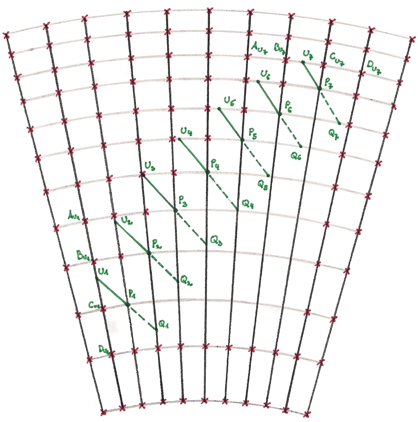
Figure 1:  One step in the iterative solution of the RTE. The rays enter at U. There, at the center P, and at the exit point Q the opacity has to be determined to perform the numerical integration on the right hand side of Eq. (9) and to get the intensity $I$ at P for the next step.

To determine the incoming intensity along this ray direction one has to interpolate the values of the required physical quantities to the points U and Q from the neighbouring grid points. This is achieved by linear interpolation. Consequently, in two dimensions 4 points are used for all quantities except for the intensity where 2 points are sufficient. Then we evaluate the equation

$$I\left(\tau_{p}\right)=I\left(\tau_{U}\right)\exp\left(\tau_{u}-\tau_{p}\right)+\int_{\tau_{U}}^{\tau_{P}}S\left(t\right)\exp\left(t-\tau_{p}\right)dt$$ (9)

numerically to get $I\left(\tau_{P}\right)$ from a quadrature rule proposed by Olson & Kunasz (1987). This procedure is repeated recursively, because after the first step one obtains just the intensity on a single new point.

The mean intensity $J$ is computed by solid angle integration. For A4 the weights are identical,

$$J=\sum_{i=1}^{N_{\mathrm{rays}}}\frac{1}{N_{\mathrm{rays}}}I\left(r^{i}\right).$$ (10)

Finally, the radiative heating rate for grey radiative transfer is given by

$$Q_{\mathrm{rad}}=4\pi\rho\chi\left(J-S\right),$$ (11)

as in the case of a non-moving grid (details on how this is handled within ANTARES can be found in Muthsam et al. (2010)).

k	r	j=0	j=1	j=2	j=3	j=4
1	-1	1
	0	1
2	-1	3/2	-1/2
	0	1/2	1/2
	1	-1/2	3/2
3	-1	$15/8$	-5/4	3/8
	0	$3/8$	3/4	-1/8
	1	$-1/8$	3/4	3/8
	2	$3/8$	-5/4	15/8
4	-1	$35/16$	-35/16	21/16	-5/16
	0	$5/16$	15/16	-5/16	1/16
	1	$-1/16$	9/16	9/16	-1/16
	2	$1/16$	-5/16	15/16	5/16
	3	$-5/16$	21/16	-35/16	35/16
5	-1	$315/128$	-105/32	189/64	-45/32	35/128
	0	$35/128$	35/32	-35/64	7/32	-5/128
	1	$-5/128$	15/32	45/64	-5/32	3/128
	2	$3/128$	-5/32	45/64	15/32	-5/128
	3	$-5/128$	7/32	-35/64	35/32	35/128
	4	$35/128$	-45/32	189/64	-105/32	315/128

Table 4:  The constants $C_{rj}$ for $k=1,\ldots,5$, $j=0,\ldots,4$ on an equidistant grid.

2.4 WENO schemes on stretched and co-moving polar grids

The differential equations solved by the ANTARES code can also be written as a system of conservation laws of the form

$$\partial_{t}U=-\nabla\cdot F\left(U\right)+S.$$ (12)

Here, $F$ is the vector-valued flux function and $S$ designates (physical or geometrical) source terms. A discretisation of the physical domain results in a centre grid $r_{i}$ and a boundary grid $r_{i+\frac{1}{2}}$, where the function $F_{i}\left(U\right)$ is computed at the cell centre and interpolated to the cell boundaries. If a simple polynomial interpolation from the centre grid to the boundary grid is used, shocks or discontinuities are either smoothed out or begin to oscillate. To avoid these problems various essentially non-oscillatory (ENO) schemes (Harten et al. (1987), Shu & Osher (1988), Shu (1997), Fedkiw et al. (1998)) have been implemented into the ANTARES code, where interpolation is done by adaptive upwinding stencils. In the ANTARES code the spatial discretisation is done for each direction separately. However, note that for a polar grid the radial and angular direction are different. In radial direction the grid is stretched while it is equidistant in angular direction. The basic idea of characteristic numerical schemes is to transform this nonlinear system into a system of nearly independent scalar equations, a typical one of the form

$$u_{t}+f(u)_{x}=0$$ (13)

(possibly with an inhomogeneity at the right hand side) and discretise each scalar equation independently and then transform the discretised system back into the original variables. Thus, for hyperbolic systems the set of conservation laws is first transformed to the eigensystem, where the equations decouple and the upwinding directions can be chosen. For the moving grid the eigenvectors are left unchanged as the grid velocity $u_{g}$ only enters into the eigenvalues:

$$\left(\begin{array}[]{l}u_{x}-u_{g}-c\\ u_{x}-u_{g}\\ u_{x}-u_{g}\\ u_{x}-u_{g}+c\end{array}\right)$$ (14)

k	r	j=0	j=1	j=2
3	-1	$\frac{a^{6}+2a^{5}+3a^{4}+3a^{3}+3a^{2}+2a+1}{a^{2}\left(a^{4}+2a^{3}+2a^{2}+2a+1\right)}$	$-\frac{a^{4}+a^{3}+a^{2}+a+1}{a^{4}\left(a^{2}+2a+1\right)}$	$\frac{a^{2}+a+1}{a^{4}\left(a^{4}+2a^{3}+2a^{2}+2a+1\right)}$
	0	$\frac{a^{2}\left(a^{2}+a+1\right)}{a^{4}+2a^{3}+2a^{2}+2a+1}$	$\frac{a^{2}+a+1}{a\left(a^{2}+2a+1\right)}$	$-\frac{1}{a\left(a^{4}+2a^{3}+2a^{2}+2a+1\right)}$
	1	$-\frac{a^{5}}{a+2a^{3}+2a^{2}+2a+1}$	$\frac{a\left(a^{2}+a+1\right)}{a+2a+1}$	$\frac{a^{2}+a+1}{a^{4}+2a^{3}+2a^{2}+2a+1}$
	2	$\frac{a^{6}\left(a^{2}+a+1\right)}{a^{4}+2a^{3}+2a^{2}+2a+1}$	$-\frac{a^{2}\left(a^{4}+a^{3}+a^{2}+a+1\right)}{a^{2}+2a+1}$	$\frac{a^{6}+2a^{5}+3a^{4}+3a^{3}+3a^{2}+2a+1}{a^{4}+2a^{3}+2a^{2}+2a+1}$

Table 5:  The constants $C_{rj}$ for $k=3$, $j=0,\ldots,2$ on the stretched grid. For better readability, $a\equiv\sqrt{q}$.

j	k=5, r=2
0	$\frac{a^{16}\left(a^{2}+a+1\right)}{a^{14}+3a^{13}+5a^{12}+8a^{11}+11a^{10}+13a^{9}+15a^{8}+16a^{7}+15a^{6}+13a^{5}+11a^{4}+8a^{3}+5a^{2}+3a+1}$
1	$-\frac{a^{8}\left(a^{4}+a^{3}+a^{2}+a+1\right)}{a^{8}+3a^{7}+4a^{6}+5a^{5}+6a^{4}+5a^{3}+4a^{2}+3a+1}$
2	$\frac{a^{2}\left(a^{8}+3a^{7}+6a^{6}+8a^{5}+9a^{4}+8a^{3}+6a^{2}+3a+1\right)}{a^{8}+4a^{7}+8a^{6}+12a^{5}+14a^{4}+12a^{3}+8a^{2}+4a+1}$
3	$\frac{a^{6}+2a^{5}+3a^{4}+3a^{3}+3a^{2}+2a+1}{a\left(a^{8}+3a^{7}+4a^{6}+5a^{5}+6a^{4}+5a^{3}+4a^{2}+3a+1\right)}$
4	$-\frac{a^{4}+a^{3}+a^{2}+a+1}{a\left(a^{14}+3a^{13}+5a^{12}+8a^{11}+11a^{10}+13a^{9}+15a^{8}+16a^{7}+15a^{6}+13a^{5}+11a^{4}+8a^{3}+5a^{2}+3a+1\right)}$

Table 6:  The constants $C_{2j}$ for $k=5$ and $r=2$.

Schemes of the ENO variety as first introduced by Harten, Engquist and Chakravarthy (Harten et al. (1987)) are based on cell averages as follows. Given the cell averages $\overline{f}_{i}\equiv f\left(r_{i}\right)$ of a function we want to find a numerical flux function $\hat{f}_{i+\frac{1}{2}}\equiv\hat{f}\left(f_{i-r},\ldots,f_{i+s}\right)$ such that the flux difference approximates the derivative $f^{\prime}\left(r_{i}\right)$ where $f$ is sufficiently smooth. The mapping from the given cell averages $\left\{\overline{f}_{j}\right\}$ in the stencil $S\left(i\right)$ to the values $\hat{f}_{i+1/2}^{-}$ is linear. Therefore, there exist constants $c_{rj}$ and $\tilde{c}_{rj}$ depending on the left shift r of the stencil $S\left(i\right)$ such that

$$\hat{f}_{i+1/2}^{-}=\sum_{j=0}^{k-1}c_{rj}\overline{f}_{i-r+j}$$ (15)

and

$$\hat{f}_{i-1/2}^{+}=\sum_{j=0}^{k-1}\tilde{c}_{rj}\overline{f}_{i-r+j}$$ (16)

where $\tilde{c}_{rj}=c_{r-1,j}$. Near discontinuities in the solution of hyperbolic conservation laws oscillations can occur because the stencil contains those discontinuities. Therefore, an adaptive stencil $S\left(i\right)$ is chosen for the interpolation of the cell boundary fluxes where the left shift r changes with the location $r_{i}$. After all the main idea of the ENO approximation is to exclude cells containing discontinuities from the stencil $S\left(i\right)$.

When using WENO (Liu et al. (1994), Jiang & Shu (1996)) instead of choosing a single stencil for the interpolation polynomial in the ENO reconstruction, a convex combination of all candidates is used to achieve the essentially non-oscillatory property. A weighted combination of adaptive stencils gives high order polynomial approximations of the divergence term $\nabla\cdot F\left(U\right)$ in smooth regions. Across discontinuities the smoothest stencil is chosen even though it is of lower order. Instead of performing a $2k-1$ order ENO scheme using stencils of that order a combination of $k$ stencils of order $k$ is used to obtain the final accuracy $2k-1$. For ANTARES the orders 3 and 5 have been considered. For a k-th order ENO scheme there are $k$ candidate stencils

$$S_{r}\left(i\right)=\left\{x_{i-r},\ldots,x_{i-r+k-1}\right\},\quad r=0,\ldots,k-1$$ (17)

which produce $k$ different reconstructions of the value $f_{i+\frac{1}{2}}$:

$$\hat{f}_{i+1/2}^{\left(r\right)}=\sum_{j=0}^{k-1}c_{rj}\overline{f}_{i-r+j},\quad r=0,\ldots,k-1.$$ (18)

The convex combination of the values $\hat{f}_{i+1/2}^{\left(r\right)}$ for the WENO approach is

$$\hat{f}_{i+1/2}=\sum_{r=0}^{k-1}w_{r}\hat{f}_{i+1/2}^{\left(r\right)},\quad r=0,\ldots,k-1$$ (19)

and is used as a new approximation for $\bar{f}_{i+1/2}$. For the weights $w_{r}\geq 0$ for all $r$ and $\sum_{r=0}^{k-1}w_{r}=1$ must be true. For a smooth function $f\left(x\right)$ there are constants $d_{r}$ so that $\sum_{r=0}^{k-1}d_{r}=1$ and

$$\hat{f}_{i+1/2}^{-}=\sum_{r=0}^{k-1}d_{r}\hat{f}_{i+1/2}^{\left(r\right)}=f\left(r_{i+1/2}\right)+O\left(\triangle r_{i}^{2k-1}\right)$$ (20)

and constants $\widetilde{d}_{r}$ so that $\sum_{k=0}^{k-1}\tilde{d}_{r}=1$ and

$$\hat{f}_{i-1/2}^{+}=\sum_{r=0}^{k-1}\tilde{d}_{r}\hat{f}_{i+1/2}^{\left(r\right)}=f\left(r_{i-1/2}\right)+O\left(\triangle r_{i}^{2k-1}\right).$$ (21)

In Liu et al. (1994) weights of the form

$$w_{r}=\frac{\alpha_{r}}{\sum_{s=0}^{k-1}\alpha_{s}}$$ (22)

with $\alpha_{r}=\frac{d_{r}}{\left(\varepsilon+\beta_{r}\right)^{2}}$ are proposed. $\varepsilon>0$ is the machine accuracy, which is introduced here to ensure that the denominator does not become zero. $\beta_{r}$ are smoothness indicators of the stencil supposed to be zero when a discontinuity is contained in the stencil. A robust choice of smoothness indicators is defined by

$$\beta_{r}=\sum_{l=1}^{k-1}\intop_{r_{i-1/2}}^{r_{i+1/2}}\Delta r_{i}^{2l-1}\left(\frac{\partial^{l}p_{r}\left(x\right)}{\partial x^{l}}\right)dx$$ (23)

where $p_{r}\left(x\right)$ is the reconstruction polynomial on the stencil $S_{r}\left(i\right)$. The smoothness indicators $\beta_{r}$ are a measure for the total variation in the interval $I_{i}$.

From a different point of view another set of approximation coefficients $C_{rj}$ (cf. Tables 4–6), of weights $w_{r}$ (cf. Table 7), of their approximations $D_{r}$ and $\tilde{D}_{r}$ and of smoothness indicators, denoted by being capitalised, can be derived. In this case the smoothness indicators for $k=3$ are:

$$\beta_{0} = Y_{0}^{2}\left(\bar{f}_{i}-\left(q+1\right)\bar{f}_{i+1}+\bar{f}_{i+2}\right)^{2}+$$ (24)

$$\left(Z_{10}\bar{f}_{i}+Z_{20}\bar{f}_{i+1}+Z_{30}\bar{f}_{i+2}\right)^{2}$$

$$\beta_{1} = Y_{1}^{2}\left(\bar{f}_{i}-\left(q+1\right)\bar{f}_{i+1}+\bar{f}_{i+2}\right)^{2}+$$

$$\left(Z_{11}\bar{f}_{i-1}+Z_{21}\bar{f}_{i}+Z_{31}\bar{f}_{i+1}\right)^{2}$$

$$\beta_{2} = Y_{2}^{2}\left(\bar{f}_{i}-\left(q+1\right)\bar{f}_{i+1}+\bar{f}_{i+2}\right)^{2}+$$

$$\left(Z_{12}\bar{f}_{i-2}+Z_{22}\bar{f}_{i-1}+Z_{32}\bar{f}_{i}\right)^{2}$$

where $Y$ and $Z_{i}$ are given in Table 8. These are also available in the ANTARES code in addition to those from (23) which are based on the approach (19)–(22) and are required for stable time integrations of our Cepheid models, as we show below. In the second approach instead of viewing $f\left(r_{i}\right)$ as cell averages and interpolating the primitive function, the flux function $f\left(r_{i}\right)$ itself is interpolated to the boundaries, leading to a different set of coefficients (Table 4). In our case a combination of stencils of length 3 with coefficients $C_{rj}$ from Table 5 yields the stencil of length 5 with coefficients $C_{2j}$ in Table 6 in smooth regions. This approach was chosen because we use a polar grid and although the spacing is that of a stretched grid in radial direction, the cell-volumes depend also on the radius as does the shape of the cells.

The approach via exact cell volumes (19)–(23) is not advisable in our case since we want to ensure conservation of the basic variables. Though the difference in area size between a rectangular cell and a polar cell is very small the difference over the whole grid is not and the ensuing error cannot be neglected. When using the original coefficients in a one-dimensional simulation e.g. energy is not preserved over a prolonged period of time: during the first 48 days of a Cepheid simulation it increases or decreases depending on various conditions. (The parameters for this Cepheid are provided Sect. 3.1). One run shows increasing values (see Fig. 2), but for a slightly larger domain and with artificial diffusivities included we obtain decreasing values. With the new set of coefficients all the conserved variables are stable (Fig. 3) when averaged over several pulsation cycles. This comparison also demonstrates that a non-conservative discretisation method is unacceptable for a realistic numerical simulation of Cepheids.

$D_{0}$	$\frac{a^{4}+a^{3}+a^{2}+a+1}{a^{10}+a^{9}+a^{8}+2a^{7}+2a^{6}+2a^{5}+2a^{4}+2a^{3}+a^{2}+a+1}$
$D_{1}$	$\frac{a^{3}\left(a^{4}+a^{3}+a^{2}+a+1\right)}{a^{8}+a^{7}+a^{5}+2a^{4}+a^{3}+a+1}$
$D_{2}$	$\frac{a^{10}}{a^{10}+a^{9}+a^{8}+2a^{7}+2a^{6}+2a^{5}+2a^{4}+2a^{3}+a^{2}+a+1}$
$\tilde{D}_{0}$	$\frac{1}{a^{10}+a^{9}+a^{8}+2a^{7}+2a^{6}+2a^{5}+2a^{4}+2a^{3}+a^{2}+a+1}$
$\tilde{D}_{1}$	$\frac{a\left(a^{4}+a^{3}+a^{2}+a+1\right)}{a^{8}+a^{7}+a^{5}+2a^{4}+a^{3}+a+1}$
$\tilde{D}_{2}$	$\frac{a^{6}\left(a^{4}+a^{3}+a^{2}+a+1\right)}{a^{10}+a^{9}+a^{8}+2a^{7}+2a^{6}+2a^{5}+2a^{4}+2a^{3}+a^{2}+a+1}$

Table 7:  Weights $D_{r}$ for $\hat{f}_{i+1/2}^{-}$ and $\tilde{D}_{r}$ for $\hat{f}_{i-1/2}^{+}$ for $k=3$.

j	$Y_{j}$	$Z_{1j}$	$Z_{2j}$	$Z_{3j}$
$0$	$\frac{\sqrt{13}}{\sqrt{3}a^{4}\left(a^{2}+1\right)}$	$\frac{a^{2}+a+1}{a^{2}\left(a+1\right)}$	$-\frac{a^{4}+a^{3}+a^{2}+a+1}{a^{4}\left(a+1\right)}$	$\frac{1}{a^{4}\left(a+1\right)}$
$1$	$\frac{\sqrt{13}}{\sqrt{3}\left(a^{2}+1\right)}$	$\frac{a^{2}}{a+1}$	$\frac{-a^{3}+1}{a\left(a+1\right)}$	$-\frac{1}{a\left(a+1\right)}$
$2$	$\frac{\sqrt{13}a^{4}}{\sqrt{3}\left(a^{2}+1\right)}$	$\frac{a^{5}}{a+1}$	$-\frac{a\left(a^{4}+a^{2}+a+1\right)}{a+1}$	$\frac{a\left(a^{2}+a+1\right)}{a+1}$

Table 8:  Coefficients for evaluating $\beta_{j}$, $j=0,1,2$, for $k=3$, Equation 24.

Figure 2:   Cepheid simulation with interpolation of the primitive function with cell averages in all directions: time evolution of radius (red) and total energy (green). Abscissa: time in days, left ordinate: radius on a linear scale relative to its initial value, right ordinate: total energy within the sphere in erg.

Figure 3:   Cepheid simulation with interpolation of the flux function and the new scheme used in all directions: time evolution of radius (red) and total energy (green). Abscissa: time in days, left ordinate: radius on a linear scale relative to its initial value, right ordinate: total energy within the sphere in erg.

Note that the formally fifth order of the WENO5 scheme (Shu, 2003) does no longer hold with the new approach. However, lack of energy conservation is not an acceptable alternative for locally higher order in smooth regions. Around discontinuities both old and new coefficient sets yield methods of second order which is also the spatial order of accuracy achieved with the new set in smooth regions. Moreover, for the one-dimensional linear advection equation with constant velocity the error coefficient is one quarter of the size of standard second order methods such as the leap-frog scheme. Leap-frog time integration, however, can cope with shocks only after modifications that degrade their accuracy even further. The main computational expense of the WENO approach is the calculation of the fluxes at each cell boundary. This occurs only once, whence the overhead due to larger interpolation stencils is negligible, as they merely use already computed information. The only important restriction originating from wider stencils in comparison with traditional second order shock capturing methods are somewhat larger minimum domain sizes for the domain decomposition approach used in the MPI parallelization in ANTARES.

2.5 Discretisation scheme for diffusion

		$q=1$
-2	$-\frac{3+6a+9a^{2}+10a^{3}+11a^{4}+10a^{5}+9a^{6}+6a^{7}+4a^{8}+2a^{9}+a^{10}}{a^{2}\left(1+a\right)^{2}\left(1+2a^{2}+2a^{4}+a^{6}\right)}$	$-\frac{71}{24}$
-1	$\frac{3+4a+5a^{2}+6a^{3}+7a^{4}+6a^{5}+6a^{6}+4a^{7}+3a^{8}+2a^{9}+a^{10}}{a^{6}\left(1+a\right)^{2}\left(1+a^{2}\right)}$	$\frac{47}{8}$
0	$-\frac{3+4a+5a^{2}+4a^{3}+4a^{4}+4a^{5}+4a^{6}+2a^{7}+a^{8}}{a^{8}\left(1+a\right)^{2}\left(1+a^{2}\right)}$	$-\frac{31}{8}$
1	$\frac{3+4a+5a^{2}+4a^{3}+4a^{4}+2a^{5}+a^{6}}{a^{8}\left(1+a\right)^{2}\left(1+2a^{2}+2a^{4}+a^{6}\right)}$	$\frac{23}{24}$
-2	$-\frac{3a^{4}+4a^{5}+5a^{6}+4a^{7}+4a^{8}+2a^{9}+a^{10}}{\left(1+a\right)^{2}\left(1+2a^{2}+2a^{4}+a^{6}\right)}$	$-\frac{23}{24}$
-1	$\frac{-2a-a^{2}+2a^{4}+2a^{5}+3a^{6}+2a^{7}+a^{8}}{a^{2}\left(1+a\right)^{2}\left(1+a^{2}\right)}$	$\frac{7}{8}$
0	$\frac{2a-a^{6}}{a^{4}\left(1+a\right)^{2}\left(1+a^{2}\right)}$	$\frac{1}{8}$
1	$-\frac{2a-a^{4}}{a^{4}\left(1+a\right)^{2}\left(1+2a^{2}+2a^{4}+a^{6}\right)}$	$-\frac{1}{24}$
-2	$\frac{2a^{9}-a^{12}}{\left(1+a\right)^{2}\left(1+2a^{2}+2a^{4}+a^{6}\right)}$	$\frac{1}{24}$
-1	$-\frac{\left(2a^{3}-a^{4}\right)\left(1+a+a^{2}\right)^{2}}{\left(1+a\right)^{2}\left(1+a^{2}\right)}$	$-\frac{9}{8}$
0	$\frac{\left(-1+2a\right)\left(1+a+a^{2}\right)^{2}}{\left(1+a\right)^{2}\left(1+a^{2}\right)}$	$\frac{9}{8}$
1	$-\frac{\left(-1+2a^{3}\right)}{\left(1+a\right)^{2}\left(1+2a^{2}+2a^{4}+a^{6}\right)}$	$-\frac{1}{24}$
-2	$\frac{-a^{12}+2a^{15}}{(1+a)^{2}(1+2a^{2}+2a^{4}+a^{6})}$	$\frac{1}{24}$
-1	$-\frac{-a^{6}+2a^{11}}{(1+a)^{2}(1+a^{2})}$	$-\frac{1}{8}$
0	$-\frac{a^{2}+2a^{3}+3a^{4}+2a^{5}+2a^{6}-a^{8}-2a^{9}}{(1+a)^{2}(1+a^{2})}$	$-\frac{7}{8}$
1	$\frac{a^{2}+2a^{3}+4a^{4}+4a^{5}+5a^{6}+4a^{7}+3a^{8}}{(1+a)^{2}(1+2a^{2}+2a^{4}+a^{6})}$	$\frac{23}{24}$
-2	$-\frac{a^{14}+2a^{15}+4a^{16}+4a^{17}+5a^{18}+4a^{19}+3a^{20}}{(1+a)^{2}(1+2a^{2}+2a^{4}+a^{6})}$	$-\frac{23}{24}$
-1	$\frac{a^{8}+2a^{9}+4a^{10}+4a^{11}+4a^{12}+4a^{13}+5a^{14}+4a^{15}+3a^{16}}{(1+a)^{2}(1+a^{2})}$	$\frac{31}{8}$
0	$-\frac{a^{4}+3a^{6}+6a^{8}+7a^{10}+5a^{12}+3a^{14}+2a^{5}+4a^{7}+6a^{9}+6a^{11}+4a^{13}}{(1+a)^{2}(1+a^{2})}$	$-\frac{47}{8}$
1	$\frac{a^{4}+2a^{5}+4a^{6}+6a^{7}+9a^{8}+10a^{9}+11a^{10}+10a^{11}+9a^{12}+6a^{13}+3a^{14}}{(1+a)^{2}(1+2a^{2}+2a^{4}+a^{6})}$	$\frac{71}{24}$

Table 9:  Discretisation of the derivative terms representing diffusion. Weights for the stencil $\left(i-2,i-1,i,i+1\right)$ for the derivatives at, from top to bottom, $i-2.5$, $i-1.5$, $i-0.5$, $i+0.5$, and $i+1.5$. The derivatives at $i-2.5$, $i-1.5$, $i+0.5$, and $i+1.5$ are only needed near the boundaries, in the inner regions the weights for $i-0.5$ are used (cf. Eq. (26)). For the equidistant grid these terms reduce to the values in the rightmost column. For better readability, $a\equiv\sqrt{q}$.

To avoid problems with conservation of mass, momentum, and energy as exemplified through Fig. 2 the interpolation of the diffusive fluxes has to be done in the same manner. The new WENO coefficients are given by Tables 5–8. Happenhofer et al. (2011) and Koch et al. (2010) discussed a differencing scheme for diffusive fluxes based on interpolating cell averages. For constant diffusivities and equidistantly spaced grid points in one dimension in a Cartesian coordinate system it recovers the well-known approximation

$$\left(-U_{i}\right)_{xx}=\frac{U_{i-2}-16\,U_{i-1}+30\,U_{i}-16\,U_{i+1}+U_{i+2}}{12\,h^{2}}$$

which is of fourth order. However, this cannot be carried over to the case of a stretched, co-moving, polar grid for the same reasons as already discussed for the WENO scheme. Plain staggered mesh interpolation of fluxes can be used instead of interpolating the cell averages in which case the derivative at $i+a-\frac{1}{2}$ is computed as

$$\left(U_{i+a-\frac{1}{2}}\right)_{r}=\frac{S_{-2}U_{i-2}+S_{-1}U_{i-1}+S_{0}U_{i}+S_{1}U_{i+1}}{r_{i+1}-r_{i}}$$ (25)

for $a=-2,...,2$. For the equidistant grid this leads to

$$\left(U_{i-\frac{1}{2}}\right)_{r}=\frac{U_{i-2}-27\,U_{i-1}+27\,U_{i}-U_{i+1}}{24\,h}$$ (26)

and

$$\left(U_{i+\frac{1}{2}}\right)_{r}=\frac{U_{i-1}-27\,U_{i}+27\,U_{i+1}-U_{i+2}}{24\,h}$$ (27)

and the second derivative is then given by

$$\left(-U_{i}\right)_{rr}=\frac{U_{i-2}-28\,U_{i-1}+54\,U_{i}-28\,U_{i+1}+U_{i+2}}{24\,h^{2}}$$ (28)

(the latter was also discussed in Koch et al. (2010) for Cartesian grids). This is a second order approximation for $\left(U_{i}\right)_{rr}$ with an error coefficient half the size of that one of the central second order difference on an equidistant grid in one dimension for the heat equation with constant diffusivity. As with the WENO scheme, the expensive part in evaluating these stencils is the computation of the cell boundary fluxes, whence the extra accuracy comes at negligible costs. Moreover, the stencils are still smaller than their WENO counterparts and thus introduce only small overheads when used in ANTARES in parallel mode. This approach can be generalised to the stretched and co-moving polar grid in a conservative manner. Details are given in Table 9 which displays these new stencils for both the interior of the domain (third panel) and for points near the (vertical) boundaries.

2.6 Subgrid scale modelling

In some of our simulations the grid refinement was aided or substituted by subgrid scale modelling. The approach we use for this purpose is based on the work of Smagorinsky (1963) and Lilly (1962). The subgrid-scale stress is written as

$$\tau_{ij}^{\mathrm{a}}=\tau_{ij}-\frac{1}{3}\delta_{ij}\tau_{kk}=-2\rho K_{m}\tilde{D}_{ij}$$ (29)

where the superscript “a” denotes the anisotropic part of a tensor and $\tilde{D}_{ij}$ is the strain rate tensor,

$$\tilde{D}_{ij}=\frac{1}{2}\left(\frac{\partial\tilde{u}_{i}}{\partial x_{j}}+\frac{\partial\tilde{u}_{j}}{\partial x_{i}}\right)-\frac{1}{3}\delta_{ij}\frac{\partial\tilde{u}_{k}}{\partial x_{k}}.$$ (30)

The eddy viscosity $K_{m}$ is given by

$$K_{m}=C\Delta^{2}\left|\tilde{D}\right|,$$ (31)

where $\Delta$ is the filter width, approximated in 2D as $\left(\Delta r_{i}\Delta y_{i}\right)^{1/2}$, and as $\left(\Delta r_{i}\Delta y_{i}\Delta z_{i}\right)^{1/3}$ in three dimensions, and $C$ is a dimensionless coefficient. This coefficient is a constant parameter which is commonly expressed through the Smagorinsky coefficient $c_{s}=C^{1/2}$. For our simulations we have chosen $c_{s}=0.2$ which is the standard value found in the literature for 2D simulations (for 3D simulations a smaller value of about 0.1 is usually preferred).

2.7 Initial and boundary conditions

We start with a one-dimensional model. For the simulations presented here such a model was kindly provided by Günter Houdek. There is no turbulent pressure included, thus the starting model set up in ANTARES is purely radiative. To accelerate the onset of pulsations the gravitational acceleration is reduced by 1% during the first few time steps. After the pulsation becomes stable and remains so for a considerable time the one-dimensional model is converted into a two-dimensional one by copying the one-dimensional model repeatedly in azimuthal direction. Slight random perturbations are applied to the new lateral momentum variable to start the truly 2D flow.

For closed boundary conditions the density is set to hydrostatic equilibrium at the top. Moreover, the conditions

$$u_{r}|_{\mathrm{top}} = u_{g}|_{\mathrm{top}}$$ (32)

$$\frac{\partial u_{\varphi}}{\partial r}|_{\mathrm{top}} = 0$$

$$\frac{\partial T}{\partial r}|_{\mathrm{top}} = 0$$

are applied at the top, and

$$u_{r}|_{\mathrm{bot}}=0$$ (33)

at the bottom. Since the star is purely radiative at the bottom the incoming energy transport is adjusted by keeping the radial component of radiative flux density $\kappa\nabla T$ at its initial value. After applying the boundary conditions, the grid is updated by moving the grid coordinates with grid velocity $\vec{u}_{g}^{n}$. The new grid velocity $\vec{u}_{g}^{n+1}$is determined as the horizontal average of the vertical velocity at the top.

3 Computational challenges

In this section we discuss, after presenting the parameters of our model, various restrictions on the timestep and their interaction with grid refinement. For model 1 the timestep varied from 0.12 to 0.16 seconds. This leads to approximately 2.5 million Runge-Kutta steps for the computation of one pulsation cycle. The simulation was carried out in MPI-mode on 256 nodes. At continuous operation this allows the calculation of one pulsation cycle every five days. For the better resolved models the computational demands were even higher.

3.1 The model parameters for the Cepheid simulations

For our Cepheid models we assume an effective temperature of $T_{\mathrm{eff}}=5125~{}\mathrm{K}$, a surface gravity of $92.48~{}\mathrm{cm\,s^{-2}}$ (i.e. $\log(g)\sim 1.97$), a luminosity $L\sim 913~{}L_{\odot}$, and a mass of $5~{}M_{\odot}$. For their composition we assume a subsolar metallicity, i.e. a hydrogen mass fraction of $X=0.7$ and a metal mass fraction of $Z=0.01$ (with the composition of $Z$ taken from Grevesse & Noels 1993). These values are well within the parameter range for which Cepheids can be observed (see Bono et al. 1994). Through a series of tests we found that these model parameters also have the advantage of reducing the numerical demands in comparison with higher luminosities and lower metallicities, for example.

The stellar radius in our models hence is 26.8 Gm (i.e. $R\sim 38.5\,R_{\odot}$), of which the outer 11.3 Gm were modelled. Three different aperture angles were used: $1^{\mathrm{o}}$, $3^{\mathrm{o}}$, and $10^{\mathrm{o}}$. The $3^{\mathrm{o}}$-models calculations were also performed with a grid refinement in the hydrogen-ionisation zone with refinement factors of 3 in radial direction and 4 in polar direction. Further details such as the radial stretching factor between vertically adjacent grid cells (innermost cells are the longest ones), the total number of grid points in each direction, and whether subgrid scale modelling is used or not, are given in Table 1. Each of these four models develops a first overtone pulsation with a period $P$ of about 3.85 days (this is slightly shorter than one would expect if the structure of the entire star were contained in the computational domain).

3.2 Time stepping

If we consider the rate at which the cell average of the basic hydrodynamical variables $\rho$, $\vec{I}$, and $e$ changes as a function of time, the largest possible timestep is determined by the CFL-condition. But in practice all our simulations were limited by the radiative timestep.

In the interior regions the diffusion approximation is valid and thus

$$\Delta t_{\mathrm{diff}}\propto\min\left(\frac{3~{}c_{\rm p}}{16\kappa\sigma T^{3}}\left(\frac{\kappa\rho}{k}\right)^{2}\right).$$ (34)

As usual, $c_{\rm p}$ stands for the heat capacity at constant pressure and $\sigma$ for the Stefan-Boltzmann constant. $k$ is essentially the inverse of the relevant, in our case therefore minimal, grid spacing, which enforces the most stringent time step restriction, i.e. $k=C/\min(\Delta r_{i},\Delta y_{i})$ with typically $1\leq C\leq 2\pi$. $C$ depends on the method used for spatial discretisation. In the code we use $C=1$ and a constant safety factor less than or equal to 1 is applied in front of the entire expression. The resulting time scale is very small in the optically thin regions. On the other hand, the time scale for relaxing a temperature perturbation of arbitrary optical thickness by radiation (assuming the radiative transfer equation where appropriate, not just the diffusion approximation) was shown by Spiegel (1957) to be, in linear approximation of the perturbation,

$$\Delta t_{\mathrm{rad}}\propto\min\left(\frac{c_{\rm p}}{16\kappa\sigma T^{3}}\left(1-\frac{\kappa\rho}{k}\mbox{\rm arccot}\frac{\kappa\rho}{k}\right)^{-1}\right).$$ (35)

Using radiative transfer in optically thin regions (and therefore applying the timestep restrictions expressed by Eq. (35) rather than Eq. (34)) results in considerably larger allowed numerical timesteps for our Cepheid. Eq. (35) leads to a minimum for $\Delta t_{\mathrm{rad}}$ in the optically thick regions where, however, $\Delta t_{\mathrm{rad}}$ converges to the time scale of radiative diffusion anyway. The timestep restrictions for our explicit methods become ever more stringent when considering finer grids. Circumventing them requires an implicit method for the time integration of the $Q_{\rm rad}$ term which we have not yet implemented.

3.3 Resolving steep gradients

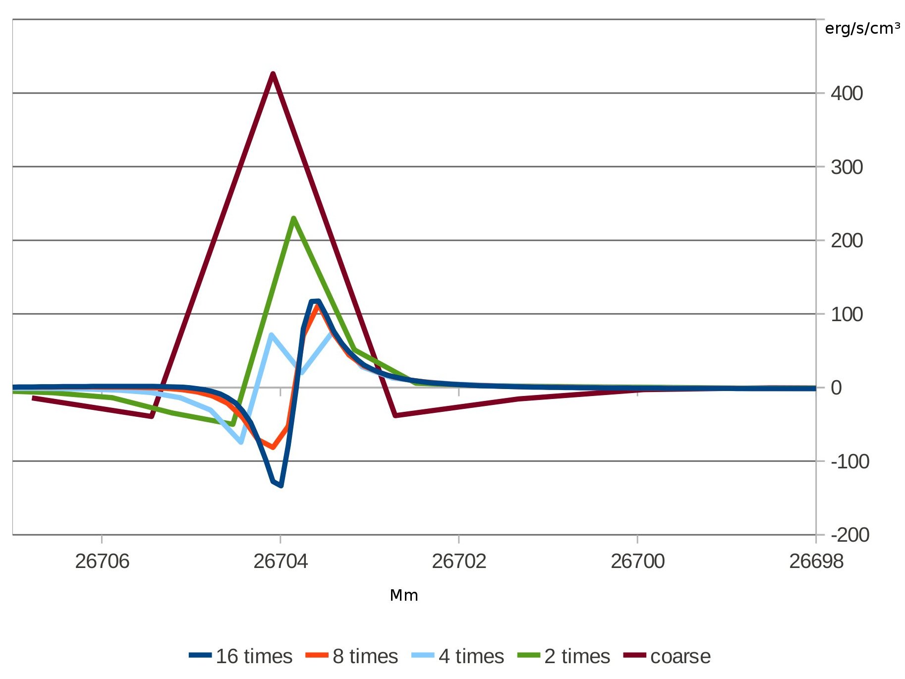
Figure 4:  The shape of $Q_{\mathrm{rad}}$ (given in erg s^-1 cm^-3) for a one-dimensional simulation at different grid refinement factors.

To resolve the steep gradients of density, temperature etc. in the hydrogen ionisation zone a resolution finer than 510 points along the radial direction is needed. For a first estimate of the required spacing we compare the pressure scale heights $H_{p}=p/|\nabla p|$ in the form $p/(\rho g)$ for models of Cepheids and the Sun in the region of interest, i.e. the stellar photosphere at a Rosseland optical depth of order unity. Substituting the pressure of a perfect gas, $p_{\mathrm{gas}}=\rho\,\mathrm{R}_{\mathrm{gas}}T/\mu$, for the pressure $p$ and the effective temperature $T_{\mathrm{eff}}$ for the temperature $T$ thus yields a ratio of pressure scale heights

$$\frac{H_{p}}{H_{p\,\odot}}=\frac{T_{\mathrm{eff}}\,\mu_{\odot}\,g_{\odot}}{T_{\mathrm{eff}\,\odot}\,\mu\,g}.$$ (36)

In our simulations of solar surface convection it was found that a minimum spacing of 20 km in radial direction is necessary to just barely resolve all basic thermodynamical variables as a function of depth. This translates to approximately 4.25 Mm for our particular Cepheid. But we must also take into account the superadiabatic gradient $\nabla-\nabla_{\rm ad}$, because we have to resolve the temperature gradient equally well as the pressure gradient. This may not be the case when considering only Eq. (36) to determine the spatial resolution of the simulation box, if the temperature gradient increases much more rapidly than it does at the superadiabatic peak of the solar convection zone. In the Sun $\max(\left(\nabla-\nabla_{\rm ad}\right)_{\odot})\approx 0.6$ (cf. Rosenthal et al. 1999). For the initial condition of the Cepheid model, which was derived using a mixing-length treatment (MLT) of convection, the maximum temperature gradient critically depends on the $\alpha$-parameter. In starting models where no turbulent pressure is included, $\max(\nabla-\nabla_{\rm ad})\approx 14$, thus the grid spacing would reduce to 0.18 Mm or a grid roughly seven times as fine as the grid used in model 1 at that location. On the other hand, if the starting model is derived with turbulent pressure included, $\max(\nabla-\nabla_{\rm ad})\approx 3.2$, and the grid of this model would only need to be refined roughly by a factor of two. While the first scenario is the only possible solution for a one dimensional, purely radiative model, there is reason to assume that in more dimensions a smaller factor can be achieved after convection has set in: the turbulent pressure caused by the flow supports the gas pressure in counteracting gravity and thus allows for lower gradients in gas pressure and temperature. The additional computation time is of course substantial: a factor of 7 in grid refinement leads to a factor $\sim 20$ for the number of temporal steps required when the timestep is limited by $\Delta t_{\mathrm{rad}}$ as given by Eq. (35). We have checked that this estimate holds at least in 1D and in Fig. 4 we present a comparison after a time evolution of 0.25 sec from the initial, static model. Obviously in 1D, a grid refinement of a factor of 2 is not enough, with a factor of 4, the radiative heating term starts to converge toward its actual shape and a factor of 8 suffices. The difference to a factor of 16 presently is not worth the extra computational costs required by such a fine resolution although it may still be large enough to lead to measurable effects in calculations of stellar spectra in future work. For our 2D simulations, where easing occurs due to the turbulent effects mentioned above, we applied a grid refinement factor of 3 in radial direction, and additional subgrid scale modelling.

4 Grid refinement

Figure 5:  The light curve for a 1D simulation on the coarse grid and on a grid having a 4 times higher resolution. Abscissa: output steps, ordinate: deviation from the average value. In both panels, the red line denotes the lightcurve while the black line indicates the radius.

For any study of the upper convection zone grid refinement is essential, as already pointed out in Sect. 3.3. To exclude effects that might result from fringing due to the grid refinement zone in an experiment with one dimensional simulations the gridspacing was reduced over the whole domain. This improved the accuracy of $Q_{\mathrm{rad}}$ and, consequently, the lightcurve smoothed out. This can be seen in Fig. 5 which also shows the results from a comparison run with the lower, original resolution. Both simulations were continued from the same initial model, an earlier state of the one-dimensional simulation on the coarser grid. Because of the higher spatial resolution the outgoing intensity becomes smaller: at the beginning the values are 30% above the average which is reached after an initial relaxation phase. The jagged lightcurve obtained with the coarse grid is totally unsuitable for comparisons with observations. This deficiency cannot be compensated by smoothing out the lightcurve since even then the average would remain too large in comparison with the simulation with lower resolution and the shape of the curve would still be different from a sufficiently resolved calculation (cf. Fig. 5). The computational resources required for the sufficiently resolved case run are unacceptably high for applications in two dimensions. Hence, the grid refinement has been modified to make it partially adaptive. The region of interest is the region where we expect to find the H-ionisation zone. Below this zone the maximum possible timestep decreases swiftly (see Fig. 6 for the inverse of $\Delta t_{\mathrm{rad}}$), therefore a finer grid can be justified only above this border. Since the location of the H-ionisation zone varies both in angular direction and with time a fixed lower boundary would invariably lead to small timesteps, and thus we developed a co-moving lower boundary. The grid refinement is done over the entire angular direction, since otherwise artifacts occur.

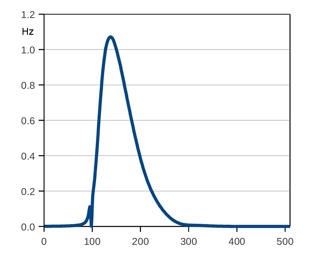
Figure 6:  Inverse of $\Delta\tau_{\mathrm{rad}}$, computed from the initial static model. Abscissa: gridpoints numbered from top to bottom, ordinate: $c_{\mathrm{cour}}/\Delta\tau_{\mathrm{rad}}$ in Hz. The H–ionisation zone is located at approximately 100, the He II–ionisation zone at approximately 300.

The most important region for grid refinement is located around the maximum of the temperature gradient. To prevent the code from finding an inappropriate maximum we also make sure that the local temperature is at least $T_{\mathrm{eff}}$ and the optical depth at least 100 at the lower border (black line in Fig. 7).

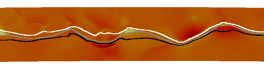
Figure 7:  Increasing optical depth in the H ionisation zone on the fine grid (model 3). Approx. 1^o wide. White line: $\tau=1$; grey line: $\tau=10$; black line $\tau=100$; plotted over the convective flux $F_{\mathrm{c}}=\left(u_{r}-\overline{u}_{r}\right)\cdot\left(\rho h-\overline{\rho h}\right)$ where $h$ denotes the enthalpy.

We now briefly describe the refinement procedure. We consider a region where the maximum temperature gradient can be found and the grid refinement factors $\mathrm{gf}(r)$ and $\mathrm{gf}(\varphi)$ are specified. If the maximum temperature gradient is outside this region, the region has to be reset. In the first step the values of the physical quantities from the coarse grid are interpolated to the fine grid to obtain the starting state for the simulation. The step for the evolution in time is calculated for both grids. This yields the number $N$ of steps on the fine grid during one step on the coarse grid. Because the calculations are limited by $\Delta t_{\mathrm{rad}}$, we get $\mathrm{gf}(r)\leq N\leq\mathrm{gf}(r)^{2}$, where $\mathrm{gf}(r)$ is the radial grid refinement factor. Since the domains are not identical, it is possible that $N$ is even smaller than $\mathrm{gf}(r)$, in which case we set $N=\mathrm{gf}(r)$. Now the “inner region” is determined. It reaches from the top of the maximum region to a few points below the location of the maximum of the temperature gradient. Grid refinement is only done in this “inner region”. For the remaining points near the superadiabatic peak the values are interpolated from the coarse grid. The lower boundary of the “inner region” is determined in every step, so that the bottom-line moves with the lower boundary of the actual H-ionisation zone. Artificial structures along this bottom line have not been observed by us in any of our simulations. Choosing, however, a top line in a similar manner we could not avoid getting artifacts: in the simulation shown in Fig. 8 such a moving top boundary was still used while this was no longer the case for the simulation shown in Fig. 9. Note that in all figures all values outside the “inner region” are only interpolated from the coarse grid.

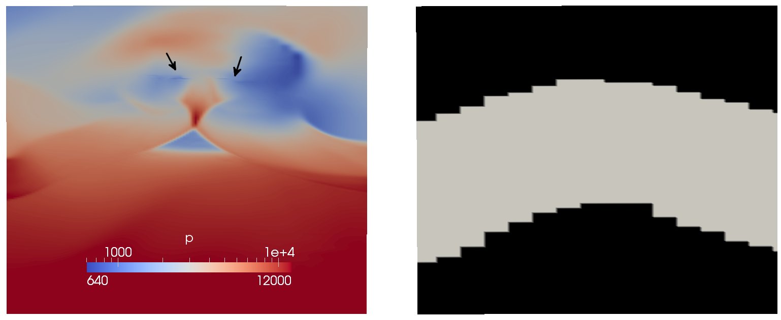
Figure 8:  Grid refinement with upper limit on the “inner region”. The left panel shows pressure, the right panel indicates the location of the grid refinement zone (grey: grid refinement zone, black: ghost cells). Note the structures in pressure (given in dyn cm^-2) displayed in the left panel as indicated by arrows which are just at the location of the upper boundary indicated in the right panel.

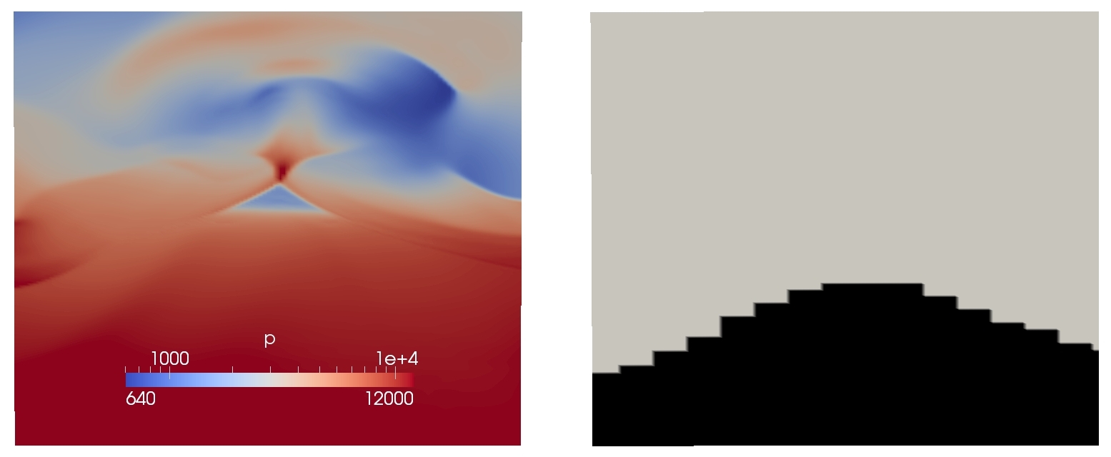
Figure 9:  Grid refinement similar to Fig. 8 but this time without upper limit on the refinement zone (“inner region”). Artifacts no longer occur.

The time steps on the fine grid are done in exactly the same way as on the coarse grid. At the beginning of each step a time interpolation yields the values in the ghost cells at the top and bottom (black region in Fig. 8 and Fig. 9) of the grid refinement zone. In angular direction they are obtained from periodic continuation. After the last step in the grid refinement region the data are projected back to the coarse grid in a conservative way.

For our two dimensional simulation (model 3) 3x4 additional grid points on each cell were used in addition to subgrid scale modelling. The resulting resolution in the critical region is $0.66~{}\mathrm{Mm}$ in radial and $1.16~{}\mathrm{Mm}$ in angular direction leading to an aspect ratio of $1:1.8$. But comparing to Fig. 4 admittedly there are still only 2 to 3 points to resolve the temperature gradient.

The uppermost panel in Fig. 10 is taken from the projection to the coarse grid and depicts the same area as the one below: the simulations both have an age of one day of stellar time. In both panels one can see the same maximum (red colour). However, not only is the convective flux already greater by a factor of 5, but there are also more convection cells in model 3 in comparison with the lower resolution model 2 and the convection cells are of an unnatural shape in model 2. Also, the maximum Mach numbers are significantly lower in model 2. The properties of the atmosphere and the differences brought about by resolution will be discussed more closely in a subsequent paper. Already from these results, however, we can state that model 2 fails by far to properly represent the hydrogen ionisation zone and the higher resolution model 3 is needed.

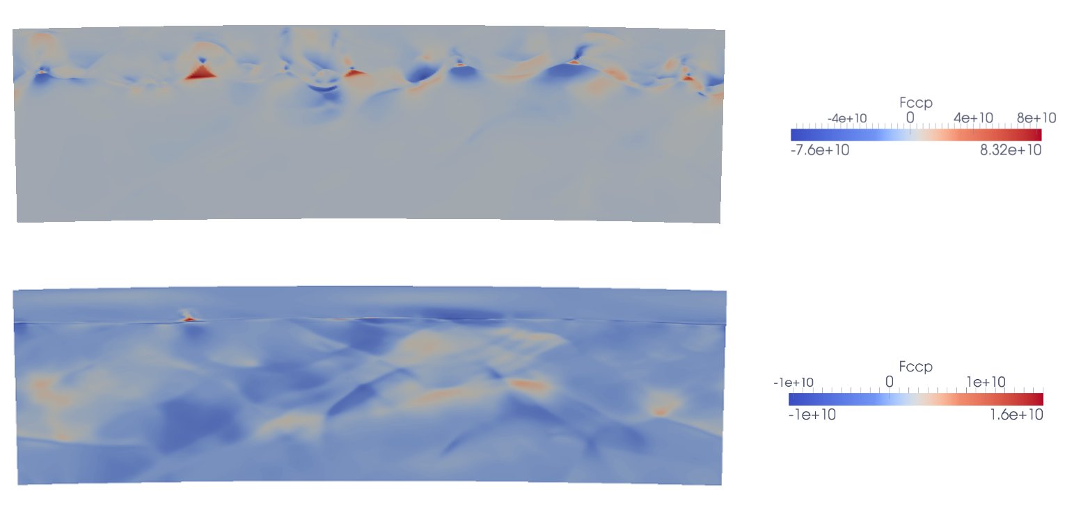
Figure 10:  Convective flux (in erg s^-1 cm^-2) in the H-ionisation zone. The upper and lower panel depict the flux in the same area and at the same time according to the models with grid refinement (model 3, upper panel) and without (model 2, lower panel). The insufficiently resolved model 2 fails to properly develop the convection zone. Note that the same colours refer to drastically different values of the convective flux in both panels. Due to projection to the coarse grid for obtaining the upper panel, the refined model is not displayed in full resolution.

5 Discussion

5.1 Comparisons and applications of the models

Among the simulations listed in Table 1 model 1 is particularly useful for astrophysical studies. The simulation domain is sufficiently wide such that the He ii zone usually contains several up- and downflow structures. Its moderate resolution is both its main strength and shortcoming. Because model 1 cannot resolve the hydrogen ionisation zone, it is very robust. Strong shock fronts develop much more rarely and, consequently, it has been easy to continue the simulation run over many pulsation cycles to provide sound statistical averages. Naturally, with this model studies on the convection-pulsation interaction have to be restricted to the role of the region around the zone of He ii ionisation. An in-depth study based on this model which investigates enthalpy fluxes and the pressure work done as a function of the pulsation phase will be presented in paper II.

Model 2 mainly serves as a reference simulation for model 3, which is derived from it through grid refinement. It has the same resolution as model 1 and differs from it only by a more narrow opening angle, thus it has no advantage over models 1 or model 3.

On the other hand, model 3 and model 4 provide two alternative ways of performing high resolution simulations which do resolve the H i and He i ionisation zone while at the same time they include the He ii ionisation zone and a sufficiently large region underneath it such that a meaningful and sufficiently accurate modelling of the radial pulsation is possible. As a consequence of its grid refinement model 3 has a wider range of applications than model 4: it offers about the same resolution combined with a much wider opening angle. Moreover, the maximum (resp. minimum) aspect ratio of the grid cells throughout the simulation domain can be reduced (kept closer to 1:1) while time step restrictions due to radiative diffusion in the layers below the superadiabatic layer can be eased as well. Finally, the He ii ionisation zone in model 4 is affected by periodicity effects along the azimuthal coordinate which are caused by the necessarily small opening angle. This clearly demonstrates the advantages of grid refinement in combination with the spherical, radially stretched and co-moving mesh used in all our simulations of Cepheids. From Fig. 10 it is evident that the dynamics at the optical surface of the Cepheid changes considerably once sufficient resolution is achieved: sharp, pronounced shock fronts appear which penetrate all the way up to the highest level of the photosphere. These phenomena will be discussed in detail in paper II. They appear in both model 3 and model 4 and the similarity of these features demonstrates that the grid refinement does not introduce any artifacts (the large, cusp like features at the optical surfaces which can be found in Fig. 8–10 are present in both model 3 and model 4 while they are hardly visible in model 2 in the lower panel of Fig. 10). Another consequence of successfully resolving the radiative cooling processes at the stellar surface is a much more realistic, relatively smooth lightcurve as shown by Fig. 5 for the one-dimensional case.

However, the new level of dynamics found in high resolution models also introduces new numerical stability problems. Indeed, for a long period of time we have been quite content with the closed boundary conditions at the top of the domain as described in Sect. 2.7. That changed once the much more vigorous convection pattern in the H i and He i ionisation zone was found in the simulations with grid refinement (see Fig. 10). When using the closed upper boundary condition as specified in Eq. (32) the faster flows and stronger shock waves generated in the highly resolved models no longer lead to a benign behaviour as observed for the weaker shocks that appear in low resolution models. As a result, high resolution models cannot successfully be continued over multiples of pulsation cycles. For such studies it is therefore necessary to develop appropriate variants of open boundary conditions.

5.2 Overcoming the problem of small time steps

To avoid unaffordable computational requirements and inefficient use of computational resources high resolution simulations of the hydrogen ionisation zone, as discussed with the examples of Fig. 4 for the one-dimensional case, require at least some terms to be treated with an implicit time integration method. The feasibility of such an approach for the case of a moving or even an adaptive grid has been shown in Dorfi (1999) for the $1\mbox{D}$ case. More recently, Viallet, Baraffe, & Walder (2011) have developed an implicit $2\mbox{D}$ code and provided test cases for problems in stellar physics.

These codes treat both the Euler equation and the diffusive term in the energy equation implicitly. For Cepheid modelling in multidimensions the situation is different from what the latter authors seem to envisage. What matters here is the stringent limitation which is imposed by the diffusive term in the energy on the timestep, if explicit time integration is used, rather than, e.g, restrictions due to the high sound speed near the bottom of the simulation domain. These limitations, which are caused by radiative diffusion, are due to unfavourable values of the physical parameters below the H+He i ionisation zone. On the other hand, the violent state of the atmosphere with strong shocks ensuing once the resolution is sufficient precludes, in this case, useful implicit time marching for the Euler equations themselves. That would be advantageous only in the case of fast flows with slowly moving features or for a low Mach number flow. For the numerical simulation of Cepheids it should hence be sufficient to implicitly advance the diffusive terms in the energy equation in time in the relevant regions. A necessary task in this respect is the development of novel Runge-Kutta methods which allow considerably larger time steps for such cases and replace the traditional schemes. Such new methods have already been constructed and tested for their efficiency by Higueras et al. (2012), where their applicability is demonstrated for the case of semiconvection, although the new schemes have actually been developed with Cepheids and A-type stars in mind.

6 Conclusions

Setting the issue of strong shocks and obvious requirements such as the need for a moving grid and spherical geometry aside Cepheid modelling in 2D and 3D is made difficult due to extremely different spatial scales which must be resolved simultaneously. This problem becomes evident only once realistic microphysics, as characterised by the equation of state and radiative conductivities, combined with realistic values for fluxes and a realistic stratification due to gravity are taken into account.

In our modified version of ANTARES we have tackled this challenge by introducing a grid in a spherical coordinate system stretched along the radial direction. The resolution is maximised by letting the grid move with the mean velocity of the uppermost domain layer and by introducing the possibility of grid refinement. The latter is essential to resolve the superadiabatic layer and the dynamical processes occurring in the photosphere such as sharp, fast moving shock fronts.

These changes in turn necessitated modifications to the WENO scheme used for the spatial discretisation of the advection operator and the pressure gradients in the dynamical equations. The new scheme discussed in this paper ensures conservation properties at the expense of a higher approximation order in smooth flow regions while it outperforms standard second order schemes due its smaller error constant. For the same reasons the discretisation of diffusion operators had to be modified accordingly. These modifications allow to achieve a high spatial resolution at a fixed level of computational costs.

A mandatory feature of a simulation code used to perform realistic numerical simulations of Cepheids is a well scaling parallelisation. For this purpose the radiative transfer scheme used in ANTARES was not only adapted to the new grid, but also implemented in a new way such that computational nodes can be distributed efficiently both along radial and azimuthal directions. This minimises overheads due to data communication and allows a cost-effective use of 256 processor cores even with grids consisting only of typically around 500 by 500 points.

Thanks to these features it has been possible to calculate a set of two-dimensional models which can be used to study the convection-pulsation interaction of Cepheids for realistic stellar parameters and realistic microphysics. A very high spatial resolution is needed to compute reliable light-curves and reliably calculate the stratification in the superadiabatic region. The grid refinement technique allows such resolution while covering a wide simulation domain and at the same time avoid the introduction of numerical artifacts.

For the time being two important problems remain on the technical and numerical side. Since unfavourably small timesteps are enforced by radiative diffusion below the H i and He i ionisation zone, the simulations are currently very expensive. A suitable implicit time integration procedure which eases these constraints is in development. Secondly, for high resolution simulations, open upper boundary conditions are required to allow stable integrations over many pulsation cycles.

The models calculated thus far are already suited to investigate the convection-pulsation interaction for the He ii-ionisation zone with realistic microphysics and to get first insights to the atmospheric structure of Cepheids with (grey) radiative transfer from $2\mbox{D}$ models. Such investigations will be presented in paper II.

References

- Aleshin (1964) Aleshin, V. I., 1964, Astronomicheskii Zhurnal, 41, 201
- Baker & Kippenhahn (1962) Baker N., Kippenhahn R., 1962, ZA, 54, 114
- Bono & Stellingwerf (1994) Bono, G., & Stellingwerf, R. F., 1994, ApJS, 93, 233
- Bono et al. (1994) Bono, G., Caputo F., Cassini S., Marconi M.,Piersanti L., & Tornambe A., 2000, ApJ, 543, 971
- Buchler (1997) Buchler, J. R., 1997, in Variables Stars and the Astrophysical Returns of the Microlensing Surveys, eds. Ferlet, R., Maillard, J.-P., 181
- Buchler & Kolláth (2000) Buchler J. R., Kolláth Z., 2000, NYASA, 898, 39
- Buchler (2009) Buchler, J. R., 2009, American Institute of Physics Conference Series, 1170, 51
- Buchler et al. (1997) Buchler, J. R., Kolláth, Z., & Marom, A., 1997, Ap&SS, 253, 139
- Carlson (1963) Carlson, B.G., 1963, in Alder, B., Fernbach, S. (eds) Methods in Computational Physics, 1
- Christy (1962) Christy, R. F., 1962, ApJ, 136, 887
- Christy (1964) Christy, R. F., 1964, Reviews of Modern Physics, 36, 555
- Cox (1980) Cox A. N., 1980, ARA&A, 18, 15
- Cox (1960) Cox J. P., 1960, ApJ, 132, 594
- Cox et al. (1966) Cox, J. P., Cox, A. N., Olsen, K. H., King, D. S., & Eilers, D. D., 1966, ApJ, 144, 1038
- Deupree (1980) Deupree, R. G., 1980, ApJ, 236, 225
- Dorfi (1999) Dorfi E. A., 1999, JCoAM, 109, 153
- Dorfi & Feuchtinger (1991) Dorfi, E. A., & Feuchtinger, M. U., 1991, A&A, 249, 417
- Fedkiw et al. (1998) Fedkiw, Merriman, Donat and Osher, July 1998, Progress in Numerical Solutions of Partial Difference Equations, Arachon, France (M.Hafez, ed.)
- Ferguson et al. (2005) Ferguson, J.W., Alexander, D.R.. Allard, F., Barman, T., Bodnarik, J.G., Hauschildt, P.H., Heffner-Wong, A., Tamanai, A., 2005, ApJ 623, 585
- Fokin (1990) Fokin A., 1990, Ap&SS, 164, 95
- Freytag et al. (2012) Freytag B., Steffen M., Ludwig H.-G., Wedemeyer-Böhm S., Schaffenberger W., Steiner O., 2012, JCoPh, 231, 919
- Gastine & Dintrans (2011) Gastine, T., & Dintrans, B., 2011, A&A, 530, L7
- Geroux & Deupree (2011) Geroux, C. M., & Deupree, R. G., 2011, ApJ, 731, 18
- Grevesse & Noels (1993) Grevesse, N., & Noels, A., N. Prantzos, E. Vangioni-Flam and M. Cassé (eds.), 1993, Symposium in Honour of Hubert Reeves’ 60th birthday: Origin and evolution of the elements, pp.15
- de Grijs (2011) de Grijs, R., 2011, An Introduction to Distance Measurement in Astronomy (Wiley)
- Happenhofer et al. (2011) Happenhofer, N., Grimm-Strele, H., Kupka, F., Löw-Baselli, B., & Muthsam, H., 2011, to appear in J. Comput. Phys. (preprint available at http://arxiv.org/abs/1112.3507)
- Harten et al. (1987) Harten, A., Enquist, B., Osher, S. & Chakravarthy, S. R., 1987, J. Comput. Phys. 71, 23
- Hertzsprung (1926) Hertzsprung, E. 1926, Bull. Astron. Inst. Netherlands, 3, 115
- Higueras et al. (2012) Higueras, I., Happenhofer, N., Koch, O., Kupka, F. 2012, submitted to SIAM J. Scientific Computing; preprint at www.asc.tuwien.ac.at/preprint/2012/asc14x2012.pdf
- Iglesias & Rogers (1996) Iglesias, C.A. & Rogers, F.J., 1996. ApJ 464, 943
- Jiang & Shu (1996) Jiang, G. S. & Shu, C.-W., 1996, J. Comput. Phys., 126, 202
- Keller (2008) Keller S. C., 2008, ApJ, 677, 483
- Koch et al. (2010) Koch, O., Kupka, F., Löw-Baselli, B., Mayrhofer, A., & Zaussinger, F., ASC Report 32/2010, ISBN 978-3-902627-03-2, Institute for Analysis and Scientific Computing, Vienna University of Technology, Wien (http://www.asc.tuwien.ac.at/preprint/2010/asc32x2010.pdf)
- Kunasz & Auer (1988) Kunasz, P. and Auer, L. H., 1988, JQSRT, 39, 67
- Kupka, Ballot, & Muthsam (2009) Kupka F., Ballot J., Muthsam H. J., 2009, CoAst, 160, 30
- Lilly (1962) Lilly, D. K., 1962, Tellus, 14 (2), 148
- Liu et al. (1994) Liu, X., Osher, S., Chan, T., 1994, J. Comput. Phys., 115, 200
- Marconi (2009) Marconi, M., 2009, American Institute of Physics Conference Series, 1170, 223
- Merriman (2003) Merriman, B., 2003, J. Scientific Computing, 19, 309
- Muthsam et al. (2010) Muthsam, H. J., Kupka, F., Löw-Baselli, B., Obertscheider, C., Langer, M. & Lenz, P., 2010, NewA, 15, 460
- Muthsam et al. (2012) Muthsam, H. J., Mundprecht, E., Kupka, F., , 2012, in preparation
- Nordlund (1982) Nordlund A., 1982, A&A, 107, 1
- Olson & Kunasz (1987) Olson, L. H and Kunasz, P., 1987, JQSRT, 38, 325
- Rogers et al. (1996) Rogers, F. J., Swenson, F. J., and Iglesias, C. A., 1996, ApJ 456, 902
- Rogers & Nayfonov (2002) Rogers F. J., Nayfonov A., 2002, ApJ, 576, 1064
- Rosenthal et al. (1999) Rosenthal, C. S., Christensen-Dalsgaard, J., Nordlund, Å., Stein, R. F., Trampedach, R., 1999, A&A, 351, 689
- Shu & Osher (1988) Shu,C.-W., Osher, S., 1988, J. Comput. Phys. 77, 439
- Shu (1997) Shu,C.-W., 1997, Technical report NASA CR-97-206253 ICASE Report No. 97-65, Institute for Computer Applications in Science and Engineering
- Shu (2003) Shu,C.-W., 2003, International Journal of Computational Fluid Dynamics, 17:2, 107
- Smagorinsky (1963) Smagorinsky, J., 1963, Mon. Weather Rev., 91, 99
- Smolec (2008) Smolec, R., 2008, CoAst, 157, 149
- Smolec & Moskalik (2008) Smolec, R., & Moskalik, P., 2008, Acta Astron., 58, 193
- Spiegel (1957) Spiegel, E. A., 1957, ApJ 126
- Tuggle & Iben (1973) Tuggle, R. S., & Iben, I., Jr., 1973, ApJ, 186, 593
- Viallet, Baraffe, & Walder (2011) Viallet M., Baraffe I., Walder R., 2011, A&A, 531, A86
- Zhevakin (1953) Zhevakin, S. A., 1953, Russ. A.J., 30, 161