The ballistic transport instability in Saturn’s rings I: formalism and linear theory

Abstract

Planetary rings sustain a continual bombardment of hypervelocity meteoroids that erode the surfaces of ring particles on time scales of $10^{5}$–$10^{7}$ years. The debris ejected from such impacts re-accretes on to the ring, though often at a slightly different orbital radius from the point of emission. This ‘ballistic transport’ leads to a rearrangement of the disk’s mass and angular momentum, and gives rise to a linear instability that generates structure on relatively large scales. It is likely that the 100-km undulations in Saturn’s inner B-ring and the plateaus and 1000-km waves in Saturn’s C-ring are connected to the nonlinear saturation of the instability. In this paper the physical problem is reformulated so as to apply to a local patch of disk (the shearing sheet). This new streamlined model helps facilitate our physical understanding of the instability, and also makes more tractable the analysis of its nonlinear dynamics. We concentrate on the linear theory in this paper, showing that the instability is restricted to a preferred range of intermediate wavenumbers and optical depths. We subsequently apply these general results to the inner B-ring and the C-ring and find that in both regions the ballistic transport instability should be near marginality, a fact that may have important consequences for its prevalence and nonlinear development. Owing to damping via self-gravity wakes, the instability should not be present in the A-ring. A following paper will explore the instability’s nonlinear saturation and how it connects to the observed large-scale structure.

1 Introduction

Like all solar-system bodies, the component particles of planetary rings must endure a hail of interplanetary meteoroids impacting at speeds on the order of $10$ km s^-1. Collectively the most erosive projectiles lie in the size range of $10^{-2}$–$10^{-1}$ cm, and it is estimated that Saturn sweeps up such particles at a rate $\gtrsim$ 10 kg s^-1 (Durisen 1984; Ip 1984; Cuzzi & Durisen 1990, hereafter CD90). Hypervelocity impacts liberate significant amounts of material from ring particles (some $10^{3}$–$10^{5}$ times the mass of each impactor), and these ejecta re-accrete on to the ring, typically at a different radial location from where they started. The exchange of ejecta between nearby regions, referred to as ‘ballistic transport’, facilitates a redistribution of mass and angular momentum on length-scales $l_{\text{th}}\sim 10-10^{3}$ km and times $t_{\mathrm{e}}\sim 10^{5}-10^{7}$ yrs that should control the large-scale evolution of Saturn’s rings. Indeed, these scalings suggest that, over the age of the solar system, $10^{2}$–$10^{4}$ times the mass of the current rings has been transported in this way.

Previous theoretical work shows that the ballistic transport process is adept at reshaping pre-existing gradients in surface density and composition. It can sharpen edges, such as those at the inner boundaries of Saturn’s A and B-rings, generate the ramp features at the feet of those edges, and influence global colour gradients (Ip 1983; Lissauer 1984; Durisen 1984; Durisen et al. 1989, hereafter D89; Durisen et al. 1992; Cuzzi & Estrada 1998; Charnoz et al. 2009). But ballistic transport can also produce structure spontaneously from a homogeneous ring via a linear instability. This ‘ballistic transport instability’ is thought to drive the 100-km wavetrains in the inner B-ring, and possibly the 100-km-wide plateaus and the low-amplitude 1000-km undulations in the C-ring (Durisen et al. 1992; Durisen 1995, hereafter D95; Colwell et al. 2009; Charnoz et al. 2009). It is to the basic theory of ballistic transport and the linear instability that this paper will be devoted.

The dynamics of ballistic transport has been successfully described by a detailed global model constructed by Durisen and coworkers in the 1980s and 1990s (D89; CD90; Durisen et al. 1992; D95; Durisen et al. 1996; Cuzzi and Estrada 1998). The model incorporates a great many physical processes, but the mathematical formalism can be unwieldy and thus potentially obscure the fundamental physics. In this paper we omit extraneous details and construct a simpler model that is easier to work with, yet remains sufficiently accurate. It is, in fact, almost identical to the leading-order Durisen formalism when expanded in the small parameter $\varrho=v_{\mathrm{e}}/v_{\mathrm{c}}\ll 1$, where $v_{\mathrm{e}}$ is the typical relative speed of the ejecta, and $v_{\mathrm{c}}$ is the orbital speed of the ring particles. (Note that Durisen and coworkers denote this ratio by $x$, which we reserve for a radial coordinate.) As a result, our model is local (the shearing sheet), and this makes the ejecta orbital dynamics easy to describe. The local formalism also permits the resulting transport terms of mass and angular momentum to be manipulated into one-dimensional integrals in convolution form. Being especially amenable to Fourier analysis, the linear theory is transparent and nonlinear simulations are comparably straightforward. Overall, the simpler formalism facilitates our physical understanding of the instability, and permits us to bring to bear the techniques of nonlinear dynamical systems. Additional physics can always be added later to sharpen the quantitative comparison with observations.

In this paper we concentrate on the linear analysis of the system. It yields a simple instability criterion, which reveals instability is facilitated, in particular, by the decrease in the ejecta emission rate near optical depths of 0.5. This drop corresponds to a transitional regime in which the disk becomes sufficiently dense that some of the liberated ejecta are reabsorbed by neighbouring particles rather than sent into orbit. In agreement with D95, we find that instability is suppressed at very low and high optical depths. But we also see that it is suppressed at very long and short wavelengths, and that unstable modes can propagate either radially inwards or outwards, depending on wavenumber. Our analysis frames the problem in terms of two dimensionless parameters: the mean optical depth $\tau_{0}$ and the ‘ballistic Prandtl number’ $\mu$, which describes the relative efficiency of mass redistribution caused by viscous stresses versus that caused by ballistic transport. Most of the uncertainties in the problem are packaged into $\mu$, which nevertheless can be tightly constrained. In the A-ring $\mu$ is relatively large, because of strong self-gravity wakes, and therefore viscous diffusion smears out potentially unstable modes. In both the inner B-ring and the C-ring $\mu$ is smaller and linear modes may grow. However, in these two cases instability is near marginality, within the uncertainties, because $\tau_{0}$ is small or large, respectively. Though instability is still likely to occur, the fact that the system is near marginality will influence its nonlinear development, potentially leading to low-amplitude saturation or bistability. A weakly nonlinear analysis of these cases, together with fully nonlinear numerical simulations, will be presented in following work.

The paper is organised as follows. In Section 2 we detail the mathematical formalism that we use to describe the ballistic transport process, culminating in the governing equation for optical depth, Eq. (22). There we also discuss the functional forms for the rate of emission, the probability of absorption and the ejecta throw distribution, which we draw from fits to the numerical calculations of CD90. The linear stability analysis follows in Section 3, in which we present growth rates and a general instability criterion with application to Saturn’s A, B, and C-rings. We discuss these results and conclude in Section 4.

2 Mathematical formalism

We consider a local model of a particulate ring, the shearing sheet (Fig. 1), which is a convenient representation of relatively small-scale dynamics in a differentially rotating disk (Goldreich & Lynden-Bell 1965). Instead of dealing with the entirety of a ring system, with its unconstrained global structure and boundary conditions, we concentrate on a small patch of disk centred on a fiducial radius $r_{0}$ and moving on a circular orbit with angular velocity $\Omega_{0}=\Omega(r_{0})$. The small patch can then be described by a Cartesian coordinate system $(x,y,z)$, with $x$ and $y$ pointing in the radial and azimuthal directions respectively, and its differential rotation represented by a combination of uniform rotation, $\Omega_{0}\,\mathbf{e}_{z}$, and linear shear, $\mathbf{v}=-S_{0}\,x\,\mathbf{e}_{y}$, where $x=r-r_{0}$. The rate of orbital shear is $S_{0}=-r_{0}(d\Omega/dr)_{0}$ and is equal to $\tfrac{3}{2}\Omega_{0}$ in a Keplerian disk. The shearing-sheet approximation introduces fractional errors of order $\lambda/r_{0}$, where $\lambda$ is the characteristic length-scale of the dynamics we want to describe. Therefore, its descriptions of 100-km-long waves in the B-ring and plateaus in the C-ring yield an error $\sim 10^{-3}$, whereas the very slow 1000-km undulations in the C-ring give $10^{-2}$. Similarly, the ballistic transport process can be described adequately by the shearing sheet, as the errors introduced scale as $l_{\text{th}}/r_{0}\sim 10^{-3}$–$10^{-2}$.

Figure 1: Diagram showing the rationale and main features of the shearing sheet model. A small patch of disk is isolated and treated as a Cartesian sheet subject to rotation and a shear flow. Terms arising from the cylindrical geometry are dropped and the coordinates $x$ and $y$ point in the radial and azimuthal direction respectively.

Let $\sigma(x,t)$ be the surface mass density of the ring, assumed from the outset to be axisymmetric. We take the particle size distribution to be fixed and assume there exists a unique relation between $\sigma$ and the normal optical thickness $\tau$. Mass conservation furnishes us with the following evolution equation for the ring:

$$\partial_{t}\sigma+\partial_{x}(\sigma\,u_{x})=\mathcal{I}-\mathcal{J},$$ (1)

where $\mathcal{I}(x,t)$ is the rate at which mass is gained, per unit area, via ballistic transport from other radii, and $\mathcal{J}(x,t)$ is the rate at which mass is lost. The radial drift speed within the ring is denoted by $u_{x}$ and is instigated by both viscous stresses and the ballistic transport of angular momentum. In the following subsections we derive a formalism that supplies us with convenient expressions for $\mathcal{I}$, $\mathcal{J}$ and the local mass flux $\sigma\,u_{x}$.

2.1 Characterising the properties of ejecta emission and absorption

2.1.1 Rate of emission, $R$

The local rate at which mass is liberated from the ring per unit area as a result of meteoritic bombardment is the erosion rate $R[\sigma(x,t)]$. This suggests a local gross erosion time $t_{\mathrm{e}}=\sigma/R[\sigma]$, which corresponds to the time it would take for the ring to be completely destroyed, in the absence of ejecta recycling. At $\tau=1$, an estimate for $t_{\mathrm{e}}$ is

$$t_{\mathrm{e}}=10^{6}\left(\frac{10^{4}}{Y}\right)\left(\frac{\sigma}{100\,\text{g cm}^{-2}}\right)\,\text{yr},$$ (2)

where the yield $Y$ is the ratio of liberated mass in a meteoroid impact to the mass of the impactor (D95). The value of $Y$ depends sensitively on the strength and composition of the ring particle’s surface, with ‘softer’ particles releasing more material and thus taking larger $Y$. Though the physical state of ring particles is poorly constrained, terrestrial laboratory experiments give $Y\approx 10^{3}$–$10^{5}$ for hard water-ice/silicate targets struck by impactors travelling at speeds $\sim 0.1$–$10$ km s^-1 (Lange & Ahrens 1987; Frisch 1992; Koschny & Grün 2001a). Note that these estimates pertain only to cratering (non-disruptive) impacts, which are the most common outcome in Saturn’s rings. Disruptive impacts produce higher effective yields, the cumulative effects of which may influence regions of the rings in which particles are smaller and hence more prone to destruction (Estrada and Durisen 2010).

2.1.2 Throw distribution, $f$

Liberated material travels in a slightly inclined and slightly eccentric Keplerian orbit that intersects the ring plane at the location of emission, $x$, and a distant location, $x+\xi$. The radial distance $\xi$ between these two locations depends on the ejection velocity, the statistics of which is summarised in a ‘throw distribution’ $f(\xi)$, normalised such that $\int f(\xi)\,\mathrm{d}\xi=1$. (Unless otherwise specified, all integrals are carried out from $-\infty$ to $\infty$.) Thus $f(\xi)\,\mathrm{d}\xi$ is the proportion of ejecta that travels a radial distance between $\xi$ and $\xi+\mathrm{d}\xi$ during its orbit. The distribution should exhibit a characteristic length-scale, the ‘throw length’ $l_{\text{th}}$. By considering the dynamics of ejecta trajectories (Subsection 2.2.1; Appendix A), we set

$$l_{\text{th}}=4\,r_{0}\,\varrho=2\times 10^{2}\,\left(\frac{v_{\mathrm{e}}}{10\,\text{m s}^{-1}}\right)\left(\frac{r_{0}}{10^{5}\,\text{km}}\right)^{3/2}\,\text{km},$$ (3)

where $\varrho=v_{\mathrm{e}}/(r_{0}\Omega)$ and here $v_{\text{e}}$ refers to the mean ejection speed. Thus $l_{\text{th}}$ is the maximum throw possible for the given mean ejection speed $v_{\text{e}}$. The magnitude of $v_{\text{e}}$, like the yield $Y$, depends closely on the physical state of the ring particle’s surface, with ‘softer’ particles possibly taking $1$ m s^-1 and ‘harder’ particles taking $100$ m s^-1 (D89; Frisch 1992; Koschny & Grün 2001b). Consequently, the small parameter $\varrho$ varies between $10^{-4}$ and $10^{-2}$, while $l_{\text{th}}$ lies between 10 and 1000 km, which encompasses the scales of the phenomena we aim to describe.

2.1.3 Probability of absorption, $P$

During their orbit, ejecta may be reabsorbed by the ring at either the radius of emission $x$ or at the distant intersection radius $x+\xi$. The probability that an ejectum is absorbed at $x+\xi$ we denote by $P[\sigma(x+\xi,t),\sigma(x,t)]$. The reason for allowing $P$ to depend on the surface density at the emitting radius $x$, as well as that at the distant radius $x+\xi$, is to account for extended excursions whereby the ejectum passes through the ring plane multiple times. This outcome is likely only in optically thin regions of the disk, and thus the second dependence may be dropped for optically thicker regions. Note that the ballistic transport of individual ejecta occurs on an orbital period $\sim 10$ hr, much less than the erosion time $t_{\mathrm{e}}$. Hence the time required to execute multiple orbits can be neglected.

2.2 Direct mass transport

Now that we have introduced $R$, $f$ and $P$ we can construct the mass gain and loss terms $\mathcal{I}$ and $\mathcal{J}$. The rate at which mass is lost from a radius $x$ is $R[\sigma(x,t)]$, while the proportion of this mass that travels to an annulus a distance $\xi$ away and of thickness $\mathrm{d}\xi$ is $f(\xi)\,\mathrm{d}\xi$. Finally, the fraction of this mass that is ultimately absorbed by this annulus is $P[\sigma(x+\xi,t),\sigma(x,t)]$. Now if we sum over all such annuli we obtain the total loss rate

$$\mathcal{J}(x,t)=R[\sigma(x,t)]\,\int P[\sigma(x+\xi,t),\sigma(x,t)]\,f(\xi)\,\mathrm{d}\xi.$$ (4)

A similar argument accounts for the total gain of mass at $x$ from all neighbouring annuli:

$$\mathcal{I}(x,t)=\int R[\sigma(x-\xi,t)]\,P[\sigma(x,t),\sigma(x-\xi,t)]\,f(\xi)\,\mathrm{d}\xi.$$ (5)

The gain and loss integrals, though potentially complicated, benefit from being one-dimensional. The integrals in the formalism of D89, on the other hand, are three dimensional and cover the two emission angles of the ejecta as well as the speed of emission. These may be more accurate but are awkward in analytic work, and costly in numerical simulations. Moreover, the three degrees of freedom in D89 should map approximately to a single throw distance $\xi$ in the case of $\varrho\ll 1$. In Appendix A we show in detail how the two formalisms join up.

2.3 Angular momentum transport

Both the ring’s viscous stresses and the radial redistribution of ejecta lead to angular momentum transport and a consequent radial drift of material. In order to calculate the mass flux associated with the slow radial motion, we need to sketch out the trajectories of the ejecta in the shearing sheet.

2.3.1 Ejecta trajectories in the shearing sheet

The orbit of a representative ejectum $[x(t),y(t),z(t)]$ in the shearing sheet obeys the Hill equations

$$\ddot{x}-2\Omega_{0}\dot{y}-3\Omega_{0}^{2}x=0,$$ (6)

$$\ddot{y}+2\Omega_{0}\dot{x}=0,$$ (7)

$$\ddot{z}+\Omega_{0}^{2}z=0,$$ (8)

where an overdot indicates a time derivative. (Throughout this paper we neglect non-Keplerian effects arising from planetary oblateness.) If the ejectum is thrown from the ring at $t=0$ from position $(0,0,0)$ (without loss of generality) and with ejection velocity $(u,v,w)$, it will undergo the following trajectory:

$$x=\frac{1}{\Omega_{0}}\left[u\,\sin\Omega_{0}t+2v\,(1-\cos\Omega_{0}t)\right],$$ (9)

$$y=\frac{1}{\Omega_{0}}\left[-2u(1-\cos\Omega_{0}t)+v(4\sin\Omega_{0}t-3\Omega_{0}t)\right],$$ (10)

$$z=\frac{w}{\Omega_{0}}\sin\Omega_{0}t.$$ (11)

The ejectum will first return to the ring plane half an orbit later, at $t=\pi/\Omega_{0}$, at position $(4v,-4u-3\pi v,0)/\Omega_{0}$ and with velocity $(-u,-7v,-w)$. If it is not reabsorbed at this point it will continue its orbit, meeting the ring plane again at $t=2\pi/\Omega_{0}$ at position $(0,-6\pi v,0)/\Omega_{0}$ with its original velocity, $(u,v,w)$. A representative trajectory is described in Fig. 2 in three dimensions and also projected in the $(x,y)$ plane. The blue dots denote ring crossings at even integer multiples of $t=\pi/\Omega$, and red dots the ring crossings at odd multiples.

In the shearing sheet context, the role of (specific) angular momentum is played by the (specific) canonical azimuthal momentum $p_{y}=\dot{y}+2\Omega_{0}x$, a quantity that is conserved in the Hill equations, and which differs from the $y$-velocity because of the Coriolis force. For a particle in a circular orbital motion at a fixed $x$ we have $\dot{y}=-\tfrac{3}{2}\Omega_{0}\,x$ and thus $p_{y}=\tfrac{1}{2}\Omega_{0}x$. The uniform radial gradient of this quantity in the shearing sheet corresponds (apart from a factor of $r_{0}$) to the local radial gradient of specific angular momentum among the family of circular Keplerian orbits. For the ejectum orbit considered above, $p_{y}=v$, which can be seen from considering the conditions at $t=0$ at the moment the particle is launched. But this value corresponds to a circular orbit located at $x=2v/\Omega_{0}$, exactly halfway between its two ring-crossing radii. The radius of this orbit is described by the dashed black line in Fig. 2b. So when an ejectum is launched, it acquires a small amount (positive or negative) of angular momentum; subsequently, it oscillates about the radius associated with its new angular momentum and is absorbed at one or other radial extremum. Translating this result into the terminology of the previous subsection, we can then say that material emitted from $x$ and with throw distance $\xi$ has $p_{y}=\tfrac{1}{2}\Omega_{0}\,(x+\xi/2)$.

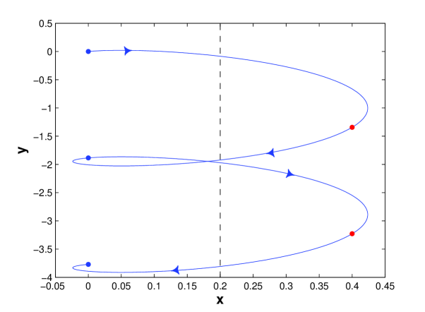
Figure 2: A representative ejectum trajectory begun at $(0,0,0)$ and evolved forward for 4 ring-plane crossings according to Eqs (9)–(11). The initial ejection speed is $(u,v,w)=(0.1,0.1,0.1)$. The first panel describes the trajectory in three dimensions with the green grid indicating the ring plane. The second panel projects this trajectory on to the $(x,y)$ plane. The dashed black line denotes the radius that corresponds to the ejectum’s angular momentum. In both figures the axes have been stretched relative to each other in order to bring out more clearly the details of the motion.

2.3.2 Radial mass drifts due to ballistic transport and viscosity

We now consider the evolution of the angular momentum analogue of the ring itself, $\sigma\,p_{y}$. The conservation law for this quantity in an axisymmetric ring is

$$\partial_{t}\left[\sigma(x,t)p_{y}\right]+\partial_{x}Q=\overline{\mathcal{K}}-\overline{\mathcal{L}},$$ (12)

where $\overline{\mathcal{K}}$ and $\overline{\mathcal{L}}$ are the rate of gain and loss of angular momentum respectively at $x$ due to ballistic transport, and $Q$ is the local momentum flux density. It is equal to

$$Q=\sigma\,u_{x}\,p_{y}-\Pi_{xy},$$ (13)

where $\Pi_{xy}$ is the $xy$ component of the viscous stress tensor. As ring material follows circular orbits predominantly, we take $p_{y}=\tfrac{1}{2}\Omega_{0}x$ from now.

The two ballistic transport terms $\overline{\mathcal{K}}$ and $\overline{\mathcal{L}}$ are straightforward to construct. Consider ejecta released at location $x$ and absorbed at $x+\xi$ in an annulus of thickness $\text{d}\xi$. The (specific) angular momentum of such ejecta is $\tfrac{1}{2}\Omega_{0}(x+\xi/2)$. As before, the rate of its emission is $R[\sigma(x,t)]$, and the proportion that travels to the annulus is $f(\xi)\,\mathrm{d}\xi$. Finally, the fraction that is absorbed at $x+\xi$ is $P[\sigma(x+\xi,t),\sigma(x,t)]$. Summing over all the neighbouring annuli yields the rate of angular momentum loss at $x$:

$$\overline{\mathcal{L}}(x,t) =R[\sigma(x,t)]\int P[\sigma(x+\xi,t),\sigma(x,t)]\,f(\xi)\,$$

$$\hskip 85.35826pt\times\tfrac{1}{2}\Omega_{0}(x+\xi/2)\,\mathrm{d}\xi.$$ (14)

The gain rate can be constructed in a similar way:

$$\overline{\mathcal{K}}(x,t) =\int R[\sigma(x-\xi,t)]\,P[\sigma(x,t),\sigma(x-\xi,t)]\,f(\xi)$$

$$\hskip 85.35826pt\times\tfrac{1}{2}\Omega_{0}\,(x-\xi/2)\,\mathrm{d}\xi.$$ (15)

The nature of the viscous stress $\Pi_{xy}$ in cold and dense particulate rings, such as Saturn’s, is nontrivial and comprises various components, each of which can deviate from the familiar Newtonian prescription (see e.g. Latter & Ogilvie 2006, 2008; Schmidt et al. 2009). In the inner rings viscous transport is dominated by the ‘collisional stress’ (Shukhman 1984; Araki & Tremaine 1986; Wisdom & Tremaine 1988), whereas stresses arising from self-gravity wakes prevail in the A-ring (Salo 1992; Daisaka et al. 2001, Yasui et al. 2012). The internal processes governing both operate on the orbital time-scale, which is much shorter than $t_{\mathrm{e}}$. It hence makes sense to treat the stress in the diffusion approximation and to introduce an effective viscosity $\nu$. The viscous mass flux then becomes

$$\Pi_{xy}=-\frac{3}{2}\Omega_{0}\nu\sigma.$$ (16)

Generally, the viscosity $\nu$ may be considered a function of $\sigma$ or optical thickness $\tau$. For simplicity, we treat $\nu$ here as a constant, although the linear theory presented in this paper is easily adapted, as we describe below, to the more realistic situation of a density-dependent viscosity.

Finally, by subtracting from Eq. (12) $\tfrac{1}{2}\Omega_{0}x$ times the mass-conservation equation (1), we can obtain an expression for the mass flux density $\sigma\,u_{x}$ that appears in the governing equation (1),

$$\sigma\,u_{x}=-\tfrac{1}{2}(\mathcal{K}+\mathcal{L})-3\partial_{x}(\nu\,\sigma).$$ (17)

This expression introduces new transport integrals defined through

$$\mathcal{K} =-\frac{4}{\Omega_{0}}(\overline{\mathcal{K}}-\tfrac{1}{2}\Omega_{0}x\,\mathcal{I})$$ (18)

and

$$\mathcal{L} =\frac{4}{\Omega_{0}}\left(\overline{\mathcal{L}}-\tfrac{1}{2}\Omega_{0}x\,\mathcal{J}\right).$$ (19)

Thus $\mathcal{K}$ and $\mathcal{L}$ are identical to $\mathcal{I}$ and $\mathcal{J}$ but with an extra factor of $\xi$ in their integrands.

Our governing equation for the surface density is then

$$\partial_{t}\sigma=\mathcal{I}-\mathcal{J}+\tfrac{1}{2}\partial_{x}(\mathcal{K}+\mathcal{L})+3\nu\partial_{x}^{2}\sigma.$$ (20)

As is well known, the viscous transport of angular momentum leads to a radial spreading of mass. The mass diffusion coefficient in a Keplerian ring resulting from a uniform kinematic viscosity is $3\nu$.

2.4 Governing dimensionless equation

Once we specify $R$, $P$, $f$ and $\nu$, we have all the ingredients to solve for the evolution of the ring. To simplify the following calculations, Eq. (1) is non-dimensionalised. Time is scaled by $t_{\mathrm{e}}$ and space by $l_{\text{th}}$. Surface density is scaled by the reference density $\sigma_{1}$. We then define the dynamical optical depth via

$$\tau(x,t)=\sigma(x,t)/\sigma_{1},$$ (21)

and so $\sigma_{1}$ is the density associated with $\tau=1$. Note that the dynamical $\tau$ can differ from the ring’s physical or photometric optical depth measured by Cassini; this is especially the case when there exist self-gravity wakes (e.g. Salo and Karjalainan 2003, Porco et al. 2008, Robbins et al. 2010). That said, in the regimes relevant to the inner B-ring and the C-ring, the discrepancy is not severe and we treat the various optical depths as approximately equal. Finally, we scale $R$ by $\sigma_{1}/t_{\mathrm{e}}$ and $f$ by $1/l_{\text{th}}$. Both $R$ and $P$ hereafter will be considered functions of $\tau$.

The scaled evolution equation for $\tau$ is

$$\partial_{t}\tau=\mathcal{I}-\mathcal{J}+\tfrac{1}{2}\partial_{x}\left(\mathcal{K}+\mathcal{L}\right)+\mu\partial_{x}^{2}\tau,$$ (22)

where we have introduced the ratio of the mass diffusion due to viscosity to the ‘ballistic diffusivity’:

$$\mu=\frac{3\nu}{l_{\text{th}}^{2}/t_{\mathrm{e}}}.$$ (23)

We emphasize that this ‘ballistic diffusivity’ is only a dimensional estimate, and will see below that ballistic transport does not in fact lead to a diffusion of mass in the conventional sense. The four ballistic transport integrals can be worked into the following forms:

$$\mathcal{I}(x,t) =\int R[\tau(x-\xi,t)]\,P[\tau(x,t),\tau(x-\xi,t)]\,f(\xi)\,\mathrm{d}\xi,$$ (24)

$$\mathcal{J}(x,t) =R[\tau(x,t)]\,\int P[\tau(x+\xi,t),\tau(x,t)]\,f(\xi)\,\mathrm{d}\xi,$$ (25)

$$\mathcal{K}(x,t) =\int R[\tau(x-\xi,t)]\,P[\tau(x,t),\tau(x-\xi,t)]\,\xi f(\xi)\,\mathrm{d}\xi,$$ (26)

$$\mathcal{L}(x,t) =R[\tau(x,t)]\int\,P[\tau(x+\xi,t),\tau(x,t)]\,\xi f(\xi)\,\mathrm{d}\xi.$$ (27)

If we make the additional approximation that $P$ depends only on the optical depth at the distant, non-emitting, radius, then we may suppress the second argument of this function. This also means that $P$ can be taken outside the integrals in the expressions for $\mathcal{I}$ and $\mathcal{K}$. The four expressions can then be written in a compact way, in which $*$ denotes a convolution integral with respect to $x$:

$$\mathcal{I}=P\cdot(R*f), \mathcal{J}=R\cdot(P*\tilde{f}),$$ (28)

$$\mathcal{K}=P\cdot(R*g), \mathcal{L}=R\cdot(P*\tilde{g}).$$ (29)

Here the function $g$ is defined by $g(\xi)=\xi f(\xi)$, and the tilde denotes a reflection, so that $f(\xi)=\tilde{f}(-\xi)$ and $g(\xi)=\tilde{g}(-\xi)$.

2.4.1 The ratio of mass transport coefficients, $\mu$

The only control parameter that appears in Eq. (22) is $\mu$, which can adopt different values depending on the dominant mode of viscous transport. In the A-ring, we expect $\nu$ to be monopolised by the action of self-gravity wakes. Analysis of density wave damping gives $\nu\approx 30-200$ cm² s^-1 (Tiscareno et al. 2007), an estimate that agrees with direct measurements of $\nu$ from $N$-body simulations of self-gravitating particles (Daisaka et al. 2001, Yasui et al. 2012). In the inner B-ring and the C-ring, however, we expect little or only moderate wake activity. In these cases, estimates from kinetic theory and simulations give $\nu\sim 0.1$ cm² s^-1 for the C-ring and $\nu\gtrsim 1.0$ cm² s^-1 for the inner B-ring (Salo et al. 2001; Schmidt et al. 2009, Yasui et al. 2012).

On the other hand, the ballistic diffusivity $l_{\text{th}}^{2}/t_{\text{e}}$ could be estimated by observing the ranges in its components from Eqs (2) and (3). If $l_{\text{th}}$ and $t_{\text{e}}$ are treated as independent, then the ballistic diffusivity is poorly constrained, its value ranging over four orders of magnitude: $l_{\text{th}}^{2}/t_{\text{e}}\sim 1-10^{4}$ cm² s^-1.

In fact, $l_{\text{th}}$ and $t_{\text{e}}$ are correlated because of the approximate relation $v_{\text{e}}\propto Y^{-1/2}$ (noted in Durisen et al. 1992). Such a relation would be consistent with a certain fraction of the impact energy being transferred to the ejecta. If we denote this fraction by $\epsilon$ we obtain:

$$\epsilon\,v_{\text{imp}}^{2}=Y\,v_{\text{e}}^{2},$$ (30)

where $v_{\text{imp}}$ is a typical impact speed. Because $l_{\text{th}}^{2}/t_{\text{e}}\propto Y\,v_{\text{e}}^{2}$, this leads to a tight bound on the ballistic diffusivity, subject to an estimate of the transfer efficiency $\epsilon$. Previous numerical and experimental studies in a variety of materials, such as basalt, glass, gabbroic anorthosite, and powdery regolith (but not ice), yield $\epsilon\sim 0.1$ in the relevant $v_{\text{imp}}$ range (O’Keefe & Ahrens 1977; Hartmann 1985; Rashev & Ahrens 2007), and we adopt this as our fiducial value. We then find

$$\frac{l_{\text{th}}^{2}}{t_{\text{e}}} \approx 1.3\times 10^{2}\left(\frac{v_{\text{imp}}}{10\,\text{km}/\text{s}}\right)^{2}\left(\frac{r}{10^{5}\,\text{km}}\right)^{3}$$

$$\hskip 85.35826pt\times\left(\frac{\sigma}{100\,\text{g}/\text{cm}^{2}}\right)^{-1}\,\text{cm}^{2}/\text{s},$$ (31)

and we expect it to take values of some $10$ cm² s^-1 and $100$ cm² s^-1 in the C-ring and in the A and B-rings respectively. Substituting these estimates into (23) yields $\mu\sim 1$ in the A-ring and $\mu\sim 0.01$ in the B and C-rings.

The behaviour of the dimensionless system (22) is thus controlled by a single tightly constrained parameter, $\mu$. But there still remains a broad spread in the physical length and time scales of the problem. Nonetheless Eqs (2) and (31) may replace (3), and therefore estimations of both the physical length $l_{\text{th}}$ and timescales $t_{\text{e}}$ of ballistic transport can be reduced to the important dependency on $Y$, the only poorly constrained parameter. For instance, setting $Y=10^{4}$ and assuming inner B-ring densities gives $t_{\text{e}}\sim 10^{6}$ years and $l_{\text{th}}\sim 500$ km.

2.4.2 Probability of absorption

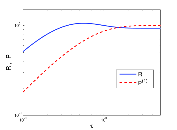
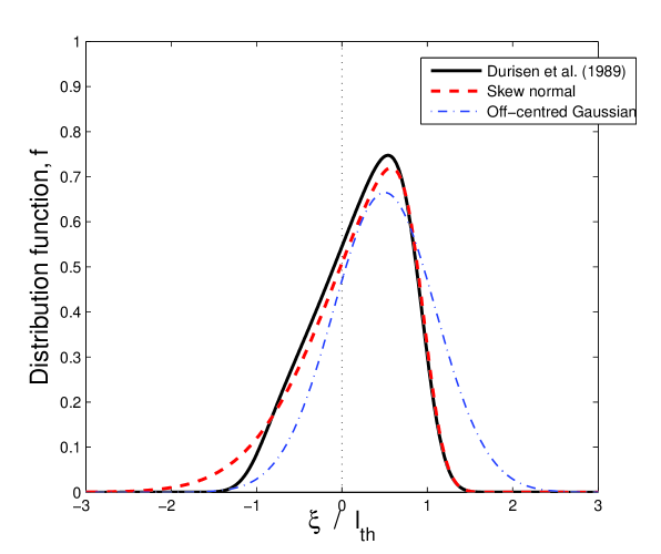
Figure 3: The first panel shows the normalised mass emission rate $R$ (blue solid line), as approximated by D89 and given by Eq. (35), and the simple absorption probability $P^{(1)}$ (red dashed line), given by Eq. (32). The second panel shows our approximation of the throw distribution $f$ as a function of throw distance $\xi$ (black solid line) as calculated by D89 (see Appendix A). In addition we plot more convenient analytic estimates: the skew-normal distribution (red dashed line) with $a=1$, $\xi_{0}=1$ and $\beta=-3.5$; and the off-centred Gaussian (blue dot-dashed lines) with $\xi_{0}=0.5$ and $a=0.6$.

This and the next subsections present expressions for the functions $P$, $f$ and $R$ and discuss their form and the relevant physics in each case. We begin by describing the probability of absorption $P$.

The fraction of ejecta that manages to pass through the ring plane on a given pass is $\text{exp}(-\tau_{\text{sl,i}})$, where $\tau_{\text{sl,i}}$ is the slant optical thickness at the radius of interception. The slant optical thickness will always be equal or greater than the normal optical depth $\tau_{\mathrm{i}}$, with the two related by $\tau_{\text{sl,i}}=\tau_{\mathrm{i}}/\cos\theta_{\text{inc}}$ where $\theta_{\text{inc}}$ is the angle of incidence of the ejecta in the frame of reference of the receiving ring particles (D89). If we next suppose that all the ejecta that manage to pass through the ring at the distant radius are then reabsorbed at the original emitting radius we may assign

$$P(\tau_{\mathrm{i}})=1-\text{exp}(-\tau_{\text{sl,i}}).$$ (32)

Where necessary, we denote this expression by $P^{(1)}$ to distinguish it from the more detailed version presented below.

However, if the emitting region is of low optical depth, an appreciable amount of material may pass through and undergo another orbit and hence another opportunity to be accreted at the distant radius. The probability that ejecta is absorbed on the second try is

$$[1-\text{exp}(-\tau_{\text{sl,i}})]\exp(-\tau_{\text{sl,e}}-\tau_{\text{sl,i}}),$$ (33)

where $\tau_{\text{sl,e}}$ is the slant optical depth of the ejecta at the emitting radius. We now sum over the formally infinite number of circuits the ejecta may complete and obtain a convergent geometric series. We can then write down the total probability of absorption:

$$P(\tau_{\mathrm{i}},\tau_{\mathrm{e}})=\frac{1-\text{exp}(-\tau_{\text{sl,i}})}{1-\text{exp}(-\tau_{\text{sl,e}}-\tau_{\text{sl,i}})}.$$ (34)

Where necessary, we denote this more advanced model by $P^{(2)}$.

To make further progress, we need to account for the angles of incidence $\theta_{\text{inc}}$ that appear in formulas (32) and (34), which should vary depending on the geometry of the orbit. Following D95, we let $\cos\theta_{\text{inc}}$ take a single ‘average’ value $\tau_{\mathrm{p}}$. We thus set $\tau_{\text{sl,i}}=\tau_{\mathrm{i}}/\tau_{\mathrm{p}}$ and $\tau_{\text{sl,e}}=\tau_{\mathrm{e}}/\tau_{\mathrm{p}}$. As is argued in D95, $\tau_{\mathrm{p}}\approx 0.5$ is a reasonably accurate approximation for a typical set of trajectories, with the error worsening in lower optical depth regions.

2.4.3 Rate of emission

In CD90 a detailed formalism is constructed whereby the intensity and angular distribution of ejecta from a ring layer may be numerically calculated. The approach borrows much from the calculation of light-scattering from a layer of particles, treating the diffuse incident intensity of meteoroids as similar to that of incident photons. The results of laboratory experiments are also used to infer the ejecta emission properties, as functions of (a) the relative velocities of a spherical ring particle and an impacting meteoroid, and (b) the angle between the impact direction and the surface normal. The single particle scattering function may then be obtained by integrating over the ejecta contributions over all points on the spherical ring particle. The ejecta distribution function proceeds directly. Finally, though the meteoroid influx is assumed to be isotropic in the heliocentric reference frame, it is aberrated in the ring reference frame because of Saturn’s and the ring particles’ orbital motion.

The results of these calculations give $R$ as a function of the optical depth at the emitting radius, and the ejecta distribution $f$ as a function of the ejection velocity vector. The former may be approximated, following D95, by the dimensionless analytic form

$$R(\tau)=0.933\left[1+\left(\frac{\tau}{\tau_{\mathrm{s}}}-1\right)\exp(-\tau/\tau_{\mathrm{s}})\right],$$ (35)

where $\tau_{\mathrm{s}}=0.28$ is a parameter. This expression is normalized such that $R(1)=1$.

In Fig. 3a we plot $R$ as a function of $\tau$. At low $\tau$ the emission rate is small because the impact rate is small. As $\tau$ increases so do the number of impacts, and consequently $R$. The drop in $R$ at $\tau_{0}\sim 0.5$ we attribute to a transition from an optically thin regime, in which almost all ejecta from a given ring particle are thrown into orbit, to an optically thick regime, in which an increasing amount of liberated ejecta is reabsorbed immediately by neighbouring ring particles. At lower $\tau$ it is possible for impact ejecta to leave the ring plane from both sides, whereas at higher $\tau$ ejecta can leave from only one side because of the intervening particles. For sufficiently large $\tau$ the emission rate relaxes to a constant value, as incoming meteoroids penetrate only to an optical depth of order unity and thus can only dislodge a fixed amount of material. The tendency for impact ejecta to be immediately accreted by neighbouring particles weakens $R$’s dependence on $\tau$, relative to $P$’s dependence (see Fig. 3a). This discrepancy plays an important role in the ring’s stability and is especially marked near $\tau=0.5$.

2.4.4 Throw distribution

The CD90 distribution function is not in the format required by our formalism as it depends on the ejection velocity: the two spherical angles that determine its orientation in the ring particle frame, $\theta$ and $\phi$, and its magnitude $v_{\mathrm{e}}$. The distribution function we have introduced, instead, depends on a single variable $\xi$, the throw distance. However, in the context of the transport integrals, an approximate mapping between $(\theta,\phi,v_{\mathrm{c}})$ and $\xi$ is possible, which allows us to translate the CD90 distribution to the $f$ used in this paper. These details are left to the Appendix. In Fig. 3b, we plot the $f$ constructed in this way alongside two convenient analytic approximations, (a) the shifted skew-normal distribution

$$f(\xi)=\frac{1}{\sqrt{2\pi}}\,\text{exp}[-(\xi-\xi_{0})^{2}/(2a^{2})]\left(1+\text{erf}\left[\beta\,(\xi-\xi_{0})\right]\right),$$ (36)

where erf is the error function, $a$ is the ‘standard deviation’, $\beta$ is the ‘shape parameter’ which measures the skewness, and the shift is $\xi_{0}$, and (b) an off-centred Gaussian,

$$f(\xi)=\frac{1}{\sqrt{2\pi a^{2}}}\text{exp}\left[-(\xi-\xi_{0})^{2}/(2a^{2})\right],$$ (37)

with shift $\xi_{0}$ and standard deviation $a$. Each of these exhibits the main feature of the realistic distribution, which is its characteristic asymmetry. Parameters that best match the computed $f$ of D89 are $a=1$, $\xi_{0}=1$, and $\beta=-3.5$ for the skew normal and $a=0.6$ and $\xi_{0}=0.5$ for the off-centred Gaussian.

The asymmetry in $f$ plays an important dynamical role, far greater than the asymmetry arising from the cylindrical effects that controlled the early studies of edge sharpening and redistribution (Ip 1983; Lissauer 1984; Durisen 1984). This outward bias is a consequence of meteoroids mainly striking the leading hemispheres of the ring particles. Ejecta are usually backscattered in these cratering impacts and thus adopt prograde orbits with $v>0$, as in Fig. 2. Ring particles suffer more impacts on their leading faces because of aberration effects that follow from the orbital motion of the ring particles around Saturn and the motion of Saturn itself through the meteoroid flux. In particular, the orbital motion of the particles gives rise to a ‘headwind’ of matter that increases both the number of impacts on their leading faces and the impact velocities $v_{\text{imp}}$. Terrestrial experiments on ice targets tell us that the ejecta yield obeys $Y\propto v_{\text{imp}}^{2}$ (see CD90), and so the ejecta population (and hence its distribution $f$) will be dominated by such prograde ejections.

2.5 Integral relations

Before applying our formalism to the question of the ring’s stability, we sketch out some general results regarding the global conservation of mass, momentum, and energy. Note that the mass and angular momentum of impacting meteorites have been neglected and thus do not appear in these balances. This is justified on the basis that $Y\gg 1$. The injection of energy, however, may be more significant and could provide a minor source of ring particle velocity dispersion. Our formalism, however, does not treat the particles’ random motion explicitly and this effect appears only through the kinematic viscosity $\nu$. See Durisen et al. (1996) for a more detailed discussion of this physics.

Suppose Eq. (20) is solved for a ring of finite radial extent on an unbounded domain, meaning that either the density is of compact support, or decays sufficiently rapidly as $x\to\pm\infty$. The following equations for the moments of the density distribution can be derived:

$$\frac{\mathrm{d}}{\mathrm{d}t}\int\sigma\,\mathrm{d}x=0,$$ (38)

$$\frac{\mathrm{d}}{\mathrm{d}t}\int\sigma\,x\,\mathrm{d}x=0,$$ (39)

$$\frac{\mathrm{d}}{\mathrm{d}t}\int\sigma\,x^{2}\,\mathrm{d}x=6\nu\int\sigma\,\mathrm{d}x.$$ (40)

These three equations can be understood as describing the evolution of the total mass, angular momentum and energy of the ring system.

It is clear that Eq. (38) expresses the conservation of mass. To derive this equation, we note that

$$\int\mathcal{I}\,\mathrm{d}x-\int\mathcal{J}\,\mathrm{d}x=0,$$ (41)

which is physically obvious and follows mathematically from a change of variables in one of the integrals.

As we have already noted, $p_{y}=\dot{y}+2\Omega_{0}x$ plays the role of specific angular momentum in the local approximation. For a simple orbital motion in which $\dot{x}=0$, $\dot{y}=-\tfrac{3}{2}\Omega_{0}x$ and $z=0$, which is the local representation of a circular orbit in the reference plane, we have $p_{y}=\tfrac{1}{2}\Omega_{0}x$. Therefore Eq. (39) expresses the conservation of angular momentum. To derive this equation, we note, using a similar change of variables, that

$$\int\mathcal{I}\,x\,\mathrm{d}x-\int\mathcal{J}\,x\,\mathrm{d}x=\int\mathcal{K}\,\mathrm{d}x=\int\mathcal{L}\,\mathrm{d}x,$$ (42)

and carry out an integration by parts for the viscous term.

The specific energy in the local approximation is

$$\tfrac{1}{2}(\dot{x}^{2}+\dot{y}^{2}+\dot{z}^{2})-\tfrac{3}{2}\Omega_{0}^{2}x^{2}+\tfrac{1}{2}\Omega_{0}^{2}z^{2},$$ (43)

which equates to $-\tfrac{3}{8}\Omega_{0}^{2}x^{2}$ for simple orbital motion. Therefore Eq. (40), which is derived in a similar way, states that the orbital energy of the ring decreases in time as a result of viscous dissipation. Ballistic transport, however, conserves mass, angular momentum and orbital energy. Eq. (40) also implies that the standard deviation of the mass distribution of a finite ring increases in time, i.e. that the ring spreads. This spreading is not (directly) counteracted by ballistic transport. Thus the edge-sharpening effects observed in simulations should be understood as a reshaping of a spreading ring feature and may be contrasted to situations where the spreading is actually halted, for instance by a shepherding satellite. In such cases Eq. (40) is modified by an external torque or angular momentum flux reversal.

The integral relations (39) and (40) do not generally hold when the equations are solved on a periodic domain because the angular momentum of material passing through the radial boundaries is not conserved.

3 Linear stability

3.1 Dispersion relation

Having set up a mathematical formalism to tackle the physics of ballistic transport, we now apply it to the question of a planetary ring’s linear stability. We reserve the problems of ring edge sharpening and structure for future work.

Consider a patch of disk in the homogeneous equilibrium state of $\tau=\tau_{0}$ with fixed $\mu$ parameter. To ease the exposition we assume for the moment that the absorption probability $P$ depends only on the local optical depth at the emitting radius, i.e. $P=P^{(1)}$. A disk of uniform $\tau$ is an equilibrium because $\mathcal{I}=\mathcal{J}$ and the local mass flux through the domain is uniform. The mass flux is in fact equal to

$$-P_{0}R_{0}\int\xi f\,\mathrm{d}\xi=-P_{0}R_{0}\langle\xi\rangle,$$ (44)

where a subscript 0 indicates evaluation at $\tau_{0}$, and $\langle\xi\rangle$ is the expected (mean) throw distance. Note that, in the homogeneous equilibrium we consider, there is no contribution to the radial drift velocity from viscous effects. Also note that if the throw distribution $f$ is completely symmetric there is no drift velocity in the equilibrium state, as $\langle\xi\rangle=0$. Ballistic transport then instigates no net angular momentum transport and hence no net radial drift.

We next superimpose on this state a small perturbation, $\hat{\tau}$. After linearising Eq. (22), we obtain

$$\partial_{t}\hat{\tau}=(R_{0}P^{\prime}_{0}-R_{0}^{\prime}P_{0})\hat{\tau}+R_{0}^{\prime}P_{0}(\hat{\tau}*f)-R_{0}P_{0}^{\prime}(\hat{\tau}*\tilde{f})$$

$$+\tfrac{1}{2}\partial_{x}\left[(R_{0}P_{0}^{\prime}+R_{0}^{\prime}P_{0})\langle\xi\rangle\hat{\tau}+R_{0}^{\prime}P_{0}(\hat{\tau}*g)+R_{0}P_{0}^{\prime}(\hat{\tau}*\tilde{g})\right]$$

$$\hskip 28.45274pt+\mu\partial_{x}^{2}\hat{\tau},$$ (45)

where a prime indicates a derivative with respect to $\tau$. Solutions exist of the form $\hat{\tau}\propto\text{e}^{st+\text{i}kx}$, where $s$ is a (complex) growth rate and $k$ a (real) wavenumber. When $\tau$ has this form, the convolutions are easily evaluated as, e.g.,

$$\hat{\tau}*f=F(k)\hat{\tau},$$ (46)

where

$$F(k)=\int f(\xi)\,\text{e}^{-\text{i}k\xi}\,\mathrm{d}\xi.$$ (47)

is the (non-unitary) Fourier transform of $f(\xi)$. This result can be seen as a consequence of the convolution theorem, since the Fourier transform of $\hat{\tau}$ is proportional to $\delta(k)$. We thus obtain the dispersion relation

$$s=R_{0}P^{\prime}_{0}-R_{0}^{\prime}P_{0}+R_{0}^{\prime}P_{0}F(k)-R_{0}P_{0}^{\prime}F(-k)$$

$$+\tfrac{1}{2}\text{i}k\left[(R_{0}P_{0}^{\prime}+R_{0}^{\prime}P_{0})\langle\xi\rangle+R_{0}^{\prime}P_{0}G(k)+R_{0}P_{0}^{\prime}G(-k)\right]$$

$$\hskip 28.45274pt-\mu k^{2},$$ (48)

where $G(k)=\text{i}F^{\prime}(k)$ is the Fourier transform of $g(\xi)$, and the prime indicates differentiation with respect to the wavenumber $k$. Since $f(\xi)$ is real, $F(-k)=\overline{F(k)}$, where the overline indicates complex conjugation. Noting further that $F(0)=1$ and $G(0)=\langle\xi\rangle$, we find

$$s=R_{0}^{\prime}P_{0}\,H(k)-R_{0}P_{0}^{\prime}\,\overline{H(k)}-\mu k^{2},$$ (49)

where

$$H(k)=F(k)-1-\frac{1}{2}k\left[F^{\prime}(k)+F^{\prime}(0)\right].$$ (50)

The first two terms in Eq. (50) come from $\mathcal{I}$ and $\mathcal{J}$ (ballistic mass transport) whereas the bracketed terms come from $\mathcal{K}$ and $\mathcal{L}$ (ballistic angular momentum transport). Note that the real part of $H$ comes from the even part of $f$, while the imaginary part of $H$ comes from the odd part of $f$. Thus linear modes will manifest as travelling waves unless the distribution $f$ is completely symmetric, as noted in D95.

3.2 Stability criterion

As a consequence of Eq. (49), the real part of $s$ is simply

$$\text{Re}(s)=\left(R_{0}^{\prime}P_{0}-R_{0}P_{0}^{\prime}\right)\text{Re}\left[H(k)\right]-\mu k^{2}.$$ (51)

This isolates in a neat mathematical way the various ingredients governing the mode’s potential growth. The first bracketed factor in the first term accounts for the combined effect of the emission and absorption rates of the ejecta; the second factor summarises the influence of the throw distribution; and the last term introduces viscous damping. It is the first term that is responsible for instability, and it must arise from either the form of the absorption/emission profile, the peculiarities of the throw distribution, or a combination of the two.

‘Realistic’ distribution functions $f$, such as those given in Section 2.3.3 and Fig. 3b, yield $\text{Re}[H(k)]<0$ for all $k$. In fact, the real part of $H$ can be positive only for exceedingly asymmetric and/or skewed distributions such as the delta function (single throw distance) considered by D95. It follows that instability is controlled by the first factor in the first term in Eq. (51). As a consequence, we can immediately derive a necessary condition for instability:

$$\frac{d\ln P}{d\tau}>\frac{d\ln R}{d\tau}.$$ (52)

This condition is satisfied when the dashed curve in Fig. 3a is steeper than the solid curve (since the plot is logarithmic). So in order to obtain a growing mode, the rate of change of absorption must outstrip the rate of emission as we increase $\tau$. This makes intuitive sense. Consider a small overdensity upon a uniform ring: as a result of the local increase in $\tau$, both the absorption $P$ and emission $R$ of ejecta will adjust. If inequality $\eqref{cond}$ holds then the ring will absorb more ejecta in relative terms than it releases. As a consequence, material will start building up at that point and the overdensity will increase, which in turn will aid the accumulation of even more mass, and so on. Similarly, in an underdense portion of an otherwise uniform ring, emission will out-compete absorption and the underdensity will be exacerbated. The drop in $R$ near $\tau=0.5$, witnessed in Fig. 3a, almost guarantees instability for $\tau\gtrsim 0.5$ because $dP/d\tau>0$.

The stability criterion (52) is only a necessary condition because we have yet to include the damping effect of viscosity. A sufficient criterion for instability, involving both $\mu$ and $\tau$, is presented in Section 3.3.2. We can, however, establish some results in the limit of small and large $k$. At very small scales, i.e. large $k$, the Riemann–Lebesgue lemma tells us that both $F(k)$ and $F^{\prime}(k)$ go to zero for realistic $f$; they do so exponentially fast if $f$ is infinitely differentiable. Hence the $-\mu k^{2}$ term in Eq. (51) dominates in this limit and modes are viscously damped, as is expected. On the other hand, on long wavelengths for which $k$ is small, a Taylor series expansion reveals that $\mathrm{Re}[H(k)]\propto k^{4}$. Therefore viscous damping ($\propto-k^{2}$) will dominate in this limit as well, and very long modes will decay. This reflects the fact that ballistic transport is weak far beyond its throw length. In summary, if the ring is unstable, growing modes are limited to a band of intermediate wavelengths, as in convection or gravitational instability. In the next subsections these results will be illustrated numerically.

In fact the Taylor expansion of $H(k)$ is

$$H(k)=-\frac{1}{12}F^{\prime\prime\prime}(0)k^{3}-\frac{1}{24}F^{\prime\prime\prime\prime}(0)k^{4}+O(k^{5}),$$ (53)

in which $F^{\prime\prime\prime}(0)=\text{i}\langle\xi^{3}\rangle$ is imaginary and $F^{\prime\prime\prime\prime}(0)=\langle\xi^{4}\rangle$ is real and positive. Terms proportional to $k$ or $k^{2}$ are absent because of cancellation between ballistic mass transport and ballistic angular momentum transport; this result is related to the fact that ballistic transport conserves the first and second moments of the surface density distribution (cf. Section 2.4). The absence of a $k^{2}$ term shows that there is no ‘ballistic diffusion’ as such, although there are dispersion and hyperdiffusion.

Before continuing on to the direct computation of growth rates, we examine the stability when the more advanced probability absorption model in Subsection 2.3.1 is adopted, and $P=P^{(2)}$. Now $P$ depends on emitting optical depth $\tau_{\mathrm{e}}$, as well as the optical depth at the intercepting radius $\tau_{\mathrm{i}}$: $P=P^{(2)}(\tau_{\mathrm{i}},\tau_{\mathrm{e}})$. The linear analysis can be worked through as before, and we find the real part of the growth rate is:

$$\text{Re}(s)=\left[R_{0}^{\prime}P_{0}-R_{0}\,\left(\frac{\partial P}{\partial\tau_{\mathrm{i}}}\right)_{0}+R_{0}\,\left(\frac{\partial P}{\partial\tau_{\mathrm{e}}}\right)_{0}\right]\text{Re}\left[H(k)\right]-\mu k^{2}.$$ (54)

Here a subscript 0 indicates evaluation at $\tau_{\mathrm{i}}=\tau_{\mathrm{e}}=\tau_{0}$. The necessary condition for instability, analogous to (52), is then

$$\frac{\partial\ln P}{\partial\tau_{\mathrm{i}}}>\frac{d\ln R}{d\tau}+\frac{\partial\ln P}{\partial\tau_{\mathrm{e}}}.$$ (55)

Because $P$ is a decreasing function of $\tau_{\mathrm{e}}$, from Eq. (34), the additional term on the right-hand side will be negative. As a result, the instability criterion will be easier to satisfy than (52). Note that the term in large square brackets in Eq. (54) is proportional to $-(A-B)$ in D95.

3.3 Specific examples

3.3.1 Growth rates

We now employ the choices of $P$, $R$ and $f$ introduced in Section 2.3 and compute growth rates explicitly. The distribution function we set equal to either the off-centred Gaussian or the skew-normal distribution, and we mainly take $P=P^{(1)}$ for simplicity. Unfortunately, the Fourier transform of the skew normal (36) is an intractable convolution. But the transform of the off-centred Gaussian (37) takes a simple form. In this case

$$F(k)=\text{exp}\left(-\tfrac{1}{2}a^{2}k^{2}-\text{i}k\xi_{0}\right),$$ (56)

and the real part of $H(k)$ is

$$\text{Re}(H)=-1+\left[(1+\tfrac{1}{2}a^{2}k^{2})\cos(k\xi_{0})\right.$$

$$\left.\hskip 56.9055pt+\tfrac{1}{2}k\xi_{0}\sin(k\xi_{0})\right]\text{e}^{-a^{2}k^{2}/2}.$$ (57)

This is negative for all $k\neq 0$ provided that $\xi_{0}/a\lesssim 4.1595$. In other words, $\text{Re}(H)<0$ unless the distribution $f$ is narrowly confined to a single throw length $\xi_{0}$. The best fit to the D89 distribution gives $\xi_{0}/a\approx 0.83$, which is well within this limit. The single throw length distribution of $\xi/a\gg 1$ was examined in D95. In this case $H$ is positive and hence the distribution can drive instability independently of the $P$ and $R$ profiles. As a result, the dispersion relation that ensues is more complicated (but unrealistic).

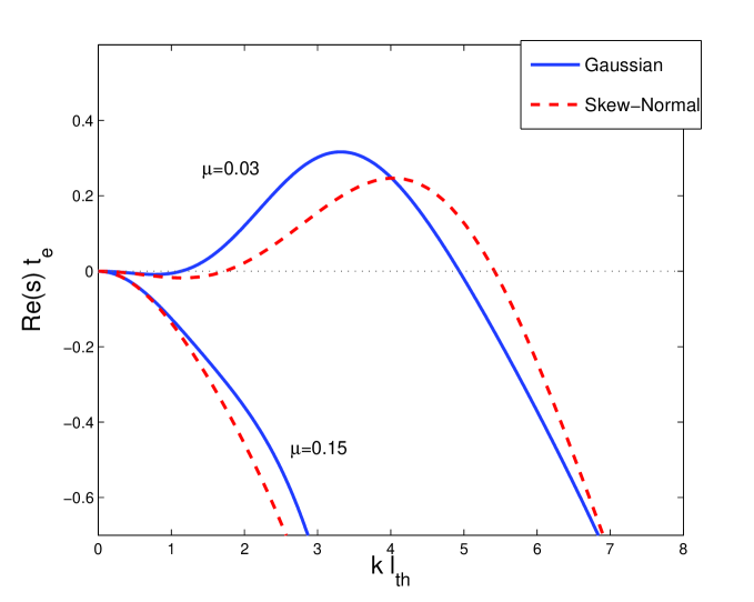
Figure 4: Real growth rates versus wavenumber $k$ for two values of $\mu$ and for two models of the distribution function $f$. The solid blue curve represents the off-centred Gaussian of (37) with $\xi_{0}=0.5$ and $a=0.6$. The dashed red curve represents the skew-normal distribution (36) with $a=\xi_{0}=1$ and $\beta=-3$. In all cases the background optical depth is $\tau=0.5$. The more viscous case $\mu=0.15$ does not exhibit instability at any $k$, but for $\mu=0.03$ instability emerges on an interval of intermediate wavenumber.

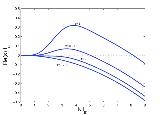
Figure 5: Real growth rates versus $k$ for various values of $\tau_{0}$. The off-centred Gaussian is used (as in in Fig. 4). The $\mu$ parameter is held fixed and is equal to 0.006. Note that instability occurs only on an intermediate range of optical depth $\tau$; both small- and large-$\tau$ rings are stable.

In Fig. 4, we plot the real part of the growth rate versus the wavenumber $k$ when $\tau_{0}=0.5$ for two values of $\mu$ and for two different distribution functions $f$. The skew-normal distribution is represented by the red dashed curve and the off-centred Gaussian by the blue solid curve. For a lower value of $\mu$, equal to 0.03, both curves exhibit growth on a characteristic range of wavenumber. Roughly, there is no growth on scales less than a throw length $l_{\text{th}}$, nor on scales longer than about $6l_{\text{th}}$. The fastest growth occurs on a scale near $(3/2)l_{\text{th}}$ with e-folding time $\sim 4t_{\mathrm{e}}$. As explained earlier, viscous diffusion dominates both long and short scales, because ballistic transport is inefficient in each limit. Note, however, that the skew-normal growth curve exhibits growth on slightly shorter lengths. Otherwise there is good qualitative agreement between the two distributions. For larger $\mu$, growth is extinguished as viscous diffusion becomes more efficient than ballistic transport and the wave modes are smoothed out before they can grow. Note that the growth rates (and their behaviour) are quantitatively consistent with the growth rates computed in D95 (his Fig. 8).

In Fig. 5, growth rates are given for different $\tau_{0}$ at a fixed $\mu$. Here only the off-centred Gaussian has been employed. The figure illustrates the fact that growth occurs only on intermediate optical depths, around $\tau_{0}\lesssim 1$: very large and very low optical depths do not exhibit instability. This reflects the relative profiles of the emission and absorption functions $R$ and $P$ given in Eqs (32) and (35). In particular, instability favours the optical depths where $R$’s rate of change with $\tau$ decreases and becomes negative.

3.3.2 Stability criterion

The stability criteria (52) and (55) are only necessary conditions because viscous diffusion has been omitted. A sufficient condition for instability must incorporate its influence and thus involve the parameter $\mu$ as well as $\tau_{0}$. From the form of the dispersion relation, marginal stability occurs when Re$(s)=d\text{Re}(s)/dk=0$. Given $\tau_{0}$, we thus have two equations to solve for a unique critical wavenumber $k$ and critical $\mu$. This is accomplished numerically, and we plot the ensuing marginal stability curve $\mu=\mu(\tau_{0})$ in the 2D parameter space of $(\mu,\tau_{0})$.

In Fig. 6 we present the marginal stability curves for the two models of the absorption function $P$, given by (32) and (34). The distribution function $f$ takes the off-centred Gaussian profile. Regions below the curves are unstable and regions above the curves are stable. The red dashed curve represents the more realistic $P^{(2)}$, which incorporates the variation in $\tau$ at both the emission and intersection radii. The blue solid curve represents the simpler $P^{(1)}$, which accounts only for $\tau$ at the intersection radius. As is clear, at moderate to large $\tau\gtrsim 1$ the two curves are much the same; this is because most ejecta in more optically thick regions undergo only one half or one orbit before being reabsorbed. The $\tau$ at the emitting radius is then unimportant. However, at low $\tau$ the two curves deviate, because ejecta undergo multiple orbits more frequently, an outcome that is not modelled by the simpler $P^{(1)}$ model. The net effect of these multiple orbits is to enhance instability. So for a given low $\tau_{0}$ the critical $\mu$ can be double that predicted by the simple model.

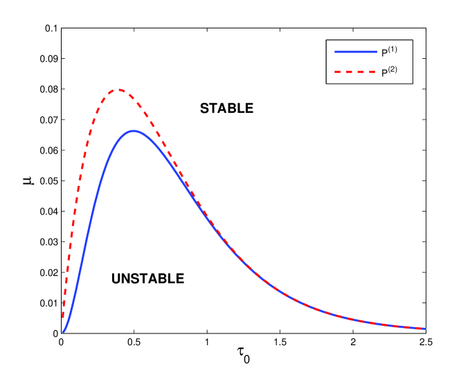
Figure 6: Curves of marginal stability in the $(\tau_{0},\mu)$ plane. The region below the curve is unstable and the region above the curve is stable. The solid blue curve corresponds to the case where the simple ‘one orbit’ model $P^{(1)}$ is employed, Eq. (32). The dashed curve represents the case where the more realistic ‘multi-orbit’ model $P^{(2)}$ is employed, Eq. (34).

Perhaps the most important result here is that the maximum $\mu$ that permits instability is remarkably low ($\approx 0.08$). Viscous diffusion must be much less than ballistic transport or else the instability is washed away. Given our estimates for $\mu$, such a low value immediately rules out the A-ring as a venue for the ballistic transport instability: we find $\mu$ is $\sim 1$ in the A-ring. On the other hand, the estimates on $\mu$ for the B and C-ring ($\sim 0.01$) suggest that instability is possible, but only barely. From Fig. 6, the critical $\mu$ is 0.032 when $\tau_{0}=1.1$ and 0.042 when $\tau=0.1$. If instability occurs in these regions then it may be near criticality, a fact that should influence its nonlinear saturation in important ways. We discuss this issue further in Section 4. Finally, we note that in the outer B-ring, where $\tau_{0}>3$, the critical $\mu$ is tiny, and instability suppressed.

Generally, for a given (sufficiently small) $\mu$ there exists an interval of $\tau$ in which instability occurs (cf. Fig. 5, and D95). Instability is suppressed at both high and low $\tau$. At high optical thicknesses, the mechanism of instability becomes weak, as both $P$ and $R$ have similar dependences on $\tau$ (cf. Fig. 3a). Over and under-densities are only mildly exacerbated, and potentially unstable modes grow too slowly to escape viscous diffusion. For similar reasons, the instability mechanism weakens at very low $\tau$. In this limit as well, both $P$ and $R$ vary similarly with $\tau$ and the first term in (51) is small as a result. Viscous damping again overwhelms potentially growing modes.

These results are consistent with the stability bounds computed in D95. If the critical effective yields $Y$ in D95 are translated to critical $\mu$ then the curves in Fig. 7 agree to within a factor of 2 (R. Durisen, private communication). This is encouraging agreement given the different distribution functions used (see the Appendix).

3.3.3 Phase speeds

Generally speaking, unstable modes manifest as travelling waves, because $s$ is complex. Only if the distribution $f$ is perfectly symmetric will modes grow in place. We define a mode’s phase speed $c_{\mathrm{p}}$ via

$$c_{\mathrm{p}}=-\frac{1}{k}\text{Im}(s)=-\frac{1}{k}\left(R\,P\right)^{\prime}_{0}\,\text{Im}[H(k)],$$ (58)

where we have used the simple model for $P$. In Fig. 7 we plot both the phase speed (red solid curve) and the real part of the growth rate (blue dashed curve) versus wavenumber $k$ for the off-centred Gaussian model of $f$.

A striking feature of $c_{\mathrm{p}}(k)$ is that it changes sign as $k$ increases. Longer growing modes propagate outwards, while shorter growing modes propagate inwards, leaving a critical $k$ at which a mode grows monotonically. Thus the direction of propagation is not strictly tied to the bias in the throw distribution $f$. Having said that, most modes (including the fastest growing) travel radially inward. In addition, as $k$ becomes large, $c_{\mathrm{p}}$ asymptotes to a constant value.

The sign reversal in the phase speed can be observed mathematically from the following argument. In the limit $k\to 0$, we have $H(k)\sim-\tfrac{1}{12}\text{i}\langle\xi^{3}\rangle k^{3}$ and so $c_{\mathrm{p}}\sim\tfrac{1}{12}(RP)^{\prime}_{0}\langle\xi^{3}\rangle k^{2}$. In the limit $k\to\infty$, we have $H(k)\sim-\tfrac{1}{2}F^{\prime}(0)k=\tfrac{1}{2}\text{i}\langle\xi\rangle k$ and so $c_{\mathrm{p}}\sim-\tfrac{1}{2}(RP)^{\prime}_{0}\langle\xi\rangle.$ The relevant throw distributions are skewed such that both $\langle\xi\rangle$ and $\langle\xi^{3}\rangle$ are positive, so a sign reversal in $c_{\mathrm{p}}$ must occur at intermediate $k$.

This behaviour can also be understood in more physical terms. Consider very short modes $k\gg 1$ with wavelengths much less than both $l_{\text{th}}$ and the throw length’s standard deviation ($a$ for the off-centred Gaussian). In such a limit, the influence of the many small undulations are ‘averaged away’. As a result, the mass transport imparts nothing to the collective motion. However, there will be a net angular momentum transport which will excite a net radial flux of material. With an outward bias to $f$ this leads to an inward drift.

Consider now a mode with wavelength much longer than $l_{\text{th}}$. Ballistic transport is then limited to relatively short distances. Suppose that mass is thrown almost entirely outward and that higher-density regions emit more mass. A density minimum will increase because it is receiving more material from the denser disk inwards to it than it can emit. Conversely, a density maximum will decrease, because it is emitting more mass than it is receiving from the (less dense) disk inwards to it. As a consequence of this differential mass transport, the entire wave-form will crawl outward, in the same direction as the throw asymmetry.

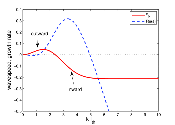
Figure 7: Phase speed $c_{\mathrm{p}}$ and real growth rate as functions of $k$, for $\tau=0.5$, $\mu=0.01$. The off-centred Gaussian is employed for $f$.

The propagation speed of the fastest growing mode is $\sim 0.2\,l_{\text{th}}/t_{\mathrm{e}}$ which lies between $0.1$ and $10$ m yr^-1. The waves move particularly slowly. This is consistent with Voyager and Cassini observations of inner B-ring structure that suggest these undulations have not travelled appreciably over a 30 year period (Colwell et al. 2009). According to the above estimate, a linear mode will have propagated between a few metres and a few hundreds of metres in that time. The upper limit is just within the range of detection, but the lower limit certainly is not. The general consistency is encouraging and suggests a potential constraint on the typical ballistic transport speed $l_{\text{th}}/t_{\mathrm{e}}$. It must be stressed, however, that the observed structures are most likely nonlinear waves which may propagate at a different speed from the linear modes.

4 Conclusion

In this paper we construct a mathematical formalism that describes the ballistic transport in planetary rings. Taking advantage of the relative smallness of the characteristic throw length $l_{\text{th}}$, which is connected directly to the parameter $\varrho\ll 1$, we employ the local shearing sheet model and manipulate the transport terms into simple 1D integrals in convolution form. The resulting main equation is simple to work with, both analytically and numerically, and its results easy to interpret. Moreover, it is almost as accurate as the classic formalism of D89, with relative errors probably of order $\varrho\sim 10^{-3}-10^{-2}$. In this paper we deploy the model on one facet of the ballistic transport process: the linear instability (D95). But it may also be used to study ramp formation and steep edges.

We derive the linear theory of the instability and apply our results to Saturn’s A, B, and C-rings. The stability analysis can be framed conveniently in terms of two parameters: $\tau_{0}$ the background optical depth and $\mu$ the ratio of mass transport coefficients due to viscous diffusion and ballistic transport. We find that, for realistic profiles of the absorption probability $P$, the ejecta emission rate $R$, and the ejecta throw distribution $f$ (D89, CD90), instability is pervasive for low and intermediate $\tau$. Actually, instability relies on the fact that $R$ increases more weakly with $\tau$ than $P$ does, and it is especially exacerbated by the drop in $R$ for $\tau\gtrsim 0.5$ (cf. Fig. 3a). Near this optical depth, a small increase in density instigates a fall in emission, and a concurrent rise in absorption. The small overdensity is hence reinforced and the process runs away. The drop in $R$ at this $\tau_{0}$ we attribute to a transition from an optically thin regime in which almost all ejecta from a given ring particle are thrown into orbit, to an optically thick regime in which increasing amount of liberated ejecta is reabsorbed immediately by neighbouring ring particles.

However, the ballistic transport instability is vulnerable to viscous diffusion which can smear out potentially growing modes. In fact, the critical $\mu$ above which instability is always extinguished is low: $\mu_{\mathrm{c}}\approx 0.08$. In the A-ring, self-gravity wakes dominate and viscous diffusion is relatively efficient; here $\mu$ takes values $\sim 1$ and instability never occurs. In the B-ring, $\mu\sim 0.01$, which precludes instability in its extremely dense outer regions, where $\tau>3$. For these large optical depths, Fig. 6 indicates $\mu_{\mathrm{c}}$ is tiny. On the other hand, the inner regions of the B-ring exhibit $\tau_{0}\approx 1$ with a corresponding critical value of $\mu_{\mathrm{c}}\approx 0.032$. Thus instability can occur but should be near marginality. The case is the same in the C-ring, where at $\tau_{0}=0.1$ we have $\mu_{\mathrm{c}}\approx 0.042$.

While we can tightly constrain the governing stability parameters, $\mu$ and mean optical depth $\tau_{0}$, the physical length and time scales of the phenomena are less easy to tie down, owing to uncertainties in the physical state of ring particle surfaces (and hence $Y$). Thus an exact determination of the preferred length-scales of the structures cannot yet be made. However, we may be able to better constrain these by matching the results of nonlinear simulations with the observed structures in detail.

The fact that instability may be near marginality in both the B and C-rings may have important dynamical consequences. On the one hand, instability may saturate at a low amplitude. Indeed the C-ring exhibits gentle undulations of 1000-km wavelength. The C-ring, however, also supports 100-km plateau structures of relatively large amplitudes at slightly larger radii (Colwell et al. 2009). Can the ballistic transport instability generate both sets of structures concurrently? This might suggest that ring properties in the C-ring vary rapidly with radius, yielding $l_{\text{th}}\sim 1000$ km near $r=80000$ km and $l_{\text{th}}\approx 100$ km at $r=90000$ km. But it is also possible that the nonlinear dynamics permits the coexistence of both dominant lengthscales; if so, detailed numerical simulations may help in showing how.

On the other hand, a system near marginality could exhibit bistability, whereby both a linearly stable homogeneous state and an active large-amplitude state are supported. In fact, the inner B-ring displays adjoining flat zones and active ‘wave zones’ between $r=93000$ km and $r=98000$ km (Colwell et al. 2009). Can we associate these two regions with the inactive (homogeneous) and active (wavelike) states of a bistable system? If so, what determines the arrangement of the states; do the states propagate into each other at a ‘front’; and at what speed would this occur? Alternatively, the ring viscosity may vary sufficiently over the inner B-ring to permit instability in some regions and not in others. The main questions are then: what is the cause of the large-scale viscosity variation and how much would it need to change to explain the observations? Because the system is near marginality here, the viscosity need not change by a great amount.

Some of these questions we hope to answer in future work where we will present the nonlinear theory and simulations of the instability. There we will exhibit the formation of wavetrain solutions, their stability to secondary modes, and the dynamics of potentially bistable regions of the disk. These various behaviours and patterns we will subsequently connect to observations.

Appendix A Connection with the D89 formalism

Most of the theoretical apparatus of D89 can be massaged into the form we present here by taking the local approximation, expanding in the small parameter $\varrho$ and retaining only leading-order terms. A number of additional assumptions then need to be made in order to connect the loss and gain integrals of D89 with the simpler versions that appear in Section 2. We sketch out these details now.

In the formalism of D89 the ballistic transport terms are generally of the form

$$\Lambda=\int_{0}^{\infty}\int_{0}^{2\pi}\int_{-1}^{1}\Theta(\tau_{\text{sl,i}})\,g(\varrho,\phi,\theta)\,d\varrho\,d\phi\,d\cos\theta,$$ (59)

where the angles $\phi$ and $\theta$ delineate the ejecta velocity orientation and $\varrho$ its magnitude (in units of $r\Omega_{0}$). The angle $\theta$ denotes the angle between the $y$ axis and the ejecta velocity, and $\phi$ the angle between $z$ axis and the projection of the velocity on to the $(x,\,z)$ plane (see Fig. 2 in D89). The function $\Theta$ is either $P$ or $R$, and $g$ is the CD90 ejection distribution function. Recall that $\tau_{\text{sl,i}}$ is the slant optical depth of the ring at the distant radius of ejecta re-intersection. The potential dependence of $P$ on $\tau_{\text{sl,e}}$ is not denoted for ease of presentation.

First we make the approximation $\tau_{\text{sl,i}}=\tau_{\mathrm{i}}/\tau_{\mathrm{p}}$, that is we treat the slant optical depth as a simple function of normal optical depth only, as assumed in Section 2.3.1. We then can set $\tau_{\mathrm{i}}=\tau(r_{\mathrm{i}})$, where $r_{\mathrm{i}}$ is the radius of the distant reintersection point. This radius may be expressed in terms of the ejecting radius $r_{\mathrm{e}}$ and $(\varrho,\phi,\theta)$:

$$r_{\mathrm{i}}=\left[\frac{1+2\varrho\cos\theta+\varrho^{2}(\cos^{2}\theta+\sin^{2}\theta\cos^{2}\phi)}{1-2\varrho\cos\theta-\varrho^{2}(\cos^{2}\theta+\sin^{2}\theta\cos^{2}\phi)}\right]r_{\mathrm{e}},$$ (60)

(see D89 and Durisen et al. 1996). Expanding in small $\varrho$ gives simply

$$r_{\mathrm{i}}=r_{\mathrm{e}}\left(1+4\varrho\cos\theta+\mathcal{O}(\varrho^{2})\right).$$ (61)

Thus if we retain only terms up to $\varrho$ then $r_{\mathrm{i}}=r_{\mathrm{i}}(\varrho,\theta)$ and hence $\Theta=\Theta(\varrho,\theta)$ and the $\phi$ dependence vanishes. All that matters now is the component of the ejecta velocity in the $y$-direction.

Next we define the throw distance

$$\xi=r_{\mathrm{i}}-r_{\mathrm{e}}=4\varrho r_{\mathrm{e}}\,\cos\theta,$$

transform the $\theta$ integral into a $\xi$ integral, and swap the order of integration. This yields the form familiar from Section 2,

$$\Lambda=\int_{-\infty}^{\infty}\Theta[\tau_{\mathrm{i}}(r_{\mathrm{i}}+\xi)]\,f(\xi)\,\mathrm{d}\xi,$$ (62)

where we have introduced the new distribution function

$$f(\xi)=\int_{0}^{2\pi}\int^{\infty}_{|\xi|/(4r_{\mathrm{e}})}\frac{g}{4\varrho r_{\mathrm{e}}}\,d\phi\,d\varrho.$$ (63)

D89 introduce an analytic approximation to the full numerical solution of $g$. It takes the form

$$g=|\sin\phi|^{1/4}\,\theta\,\text{exp}(-\theta^{1.3})\,h(\varrho),$$ (64)

where $h$ is a yet to be specified function of $\varrho$. Using this estimate, the $\phi$ integral in (63) can be done immediately, leaving the sole $\varrho$ integral. The simplest choice for $h$ is a delta function $\delta(\varrho-\varrho_{\mathrm{c}})$, for fixed $\varrho_{\mathrm{c}}$. This means that all ejecta are released with the same speed. This then accounts for the $\varrho$ integral and we obtain

$$f\propto\cos^{-1}(\xi/l_{\text{th}})\,\text{exp}[-(\cos^{-1}(\xi/l_{\text{th}}))^{1.3}],$$ (65)

where we have set $l_{\text{th}}=4\varrho_{\mathrm{c}}r_{\mathrm{e}}$. A more realistic choice but with the same basic properties is

$$h(\varrho)=\varrho\,\text{exp}[-(\varrho-\varrho_{\mathrm{c}})^{2}/(2a_{\mathrm{D}}^{2})],$$ (66)

for some (narrow) dispersion $a_{\mathrm{D}}^{2}$. The $\varrho$ integral in (63) then must be accomplished numerically. The resulting function is plotted in Fig. 3b with $a_{\mathrm{D}}=0.2$. Note that in D95, $g$ is mainly taken to be a distribution uniform over hemispheres with $h$ a truncated power law, derived from hypervelocity experimental data (Durisen et al. 1992).

References

- (1) Araki, S., Tremaine, S., 1986. Icarus, 65, 83.
- (2) Charnoz, S., Dones, L., Esposito, L. W., Estrada, P. R., Hedman, M. M., 2009. In: Dougherty, M. K., Esposito, L. W., Krimigis, S. M. (eds.), Saturn from Cassini-Huygens, Springer, Dordrecht Netherlands, p537.
- (3) Colwell, J. E., Esposito, L. W., Sremcevic, M., Stewart, G. R., McClintock, W. E., 2007. Icarus, 190, 127.
- (4) Colwell, J. E., Nicholson, P. D., Tiscareno M. S., Murray, C. D., French, R. G., Marouf, E. A., 2009. In: Dougherty, M. K., Esposito, L. W., Krimigis, S. M. (eds.), Saturn from Cassini-Huygens, Springer, Dordrecht Netherlands, p375.
- (5) Cuzzi, J. N., Durisen, R. H., 1990. Icarus, 84, 467. (CD90)
- (6) Cuzzi, J. N., Estrada, P. R., 1998. Icarus, 132, 1.
- (7) Daisaka, H., Tanaka, H., Ida, S., 2001. Icarus, 154, 296.
- (8) Durisen, R. H., 1984. In: Greenberg, R., Brahic, A., (Eds), Planetary Rings, University if Arizona Press, Tucson, p416.
- (9) Durisen, R. H., 1995. Icarus, 115, 66. (D95)
- (10) Durisen, R. H., Cramer, N. L., Murphy, B. W., Cuzzi, J. N., Mullikin, T. L., Cederbloom, S. E., 1989. Icarus, 80, 136. (D89)
- (11) Durisen, R. H., Bode, P. W., Cuzzi, J. N., Cederbloom, S. E., Murphy, B. W., 1992. Icarus, 100, 364.
- (12) Durisen, R. H., Bode, P. W., Dyck, S. G., Cuzzi, J. N., Dull, J. D., White, J. C., 1996. Icarus, 124, 220.
- (13) Estrada, P. R¿, Durisen, R. H., 2010. In: Lunar and Planetary Science Conference, 41st, The Woodlands, Texas, p2686.
- (14) Frisch W., 1992. In: McDonnell, J. A. M. (Ed), Hypervelocity Impacts in Space, University of Kent Press, Canterbury, p7.
- (15) Goertz, C. K., Morfill, G., 1988. Icarus, 74, 325.
- (16) Goldreich, P., Lynden-Bell, D., 1965. MNRAS, 130, 125.
- (17) Hartmann, W. K., 1985. Icarus, 63, 69.
- (18) Ip, W.-H, 1983. Icarus, 54, 253.
- (19) Ip, W.-H, 1984. Icarus, 60, 547.
- (20) Koschny D., Grün E., 2001a. Icarus, 154, 391.
- (21) Koschny D., Grün E., 2001b. Icarus, 154, 402.
- (22) Lange, M. A., Ahrens, T. J., 1987. Icarus, 69, 506.
- (23) Latter, H. N., Ogilvie, G. I., 2006. Icarus, 184, 498.
- (24) Latter, H. N., Ogilvie, G. I., 2008. Icarus, 195, 725.
- (25) Lissauer, J. J., 1984. Icarus, 57, 63.
- (26) O’Keefe, J. D., Ahrens, T. J., 1977. In: Lunar Science Conference, 8th, Houston, Texas, Proceedings. New York, Pergamon Press, p3357.
- (27) Porco, C. C. and 34 colleagues, 2005. Science, 307, 1226
- (28) Porco, C. C., Weiss, J. W., Richardson, D. C., Dones, L., Quinn, T., Throop, H., 2008. AJ, 136, 2172.
- (29) Rashev, M. V., Ahrens, T. J., 2007. In: Lunar and Planetary Science Conference, 38th, League City, Texas, p2058.
- (30) Robbins, S. J., Stewart, G. R., Lewis, M. C., Colwell, J. E., Sremcevic, M., 2010. Icarus, 206, 431.
- (31) Salo, H., 1992a. Nature, 359, 619.
- (32) Salo, H., Karjalainan, R., 2003. Icarus, 164, 428.
- (33) Salo, H., Schmidt, J., Spahn, F., 2001. Icarus, 153, 295.
- (34) Schmidt, J., Ohtsuki, K., Rappaport, N., Salo, H., Spahn, F., 2009. In: Dougherty, M. K., Esposito, L. W., Krimigis, S. M. (eds.), Saturn from Cassini-Huygens, Springer, Dordrecht Netherlands, p413.
- (35) Shan, L.-H., Goertz, C. K., 1991. ApJ, 367, 350.
- (36) Shukhman, I. G., 1984. Soviet Astronomy, 28, 574.
- (37) Tiscareno, M. S., 2007. Icarus, 189, 14.
- (38) Wisdom, J., Tremaine, S., 1988. The Astronomical Journal, 95, 925.
- (39) Yasui, Y., Ohtsuki, K., Daisaka, H., 2012. AJ, 143, 110.