Prominence plasma diagnostics through EUV absorption

Abstract

In this paper we introduce a new diagnostic technique that uses prominence EUV and UV absorption to determine the prominence plasma electron temperature and column emission measure, as well as He/H relative abundance; if a realistic assumption on the geometry of the absorbing plasma can be made, this technique can also yield the absorbing plasma electron density. This technique capitalizes on the absorption properties of Hydrogen and Helium at different wavelength ranges and temperature regimes. Several cases where this technique can be successfully applied are described. This technique works best when prominence plasmas are hotter than 15,000 K and thus it is ideally suited for rapidly heating erupting prominences observed during the initial phases of coronal mass ejections. An example is made using simulated intensities of 4 channels of the SDO/AIA instrument. This technique can be easily applied to existing observations from almost all space missions devoted to the study of the solar atmosphere, which we list.

1 Introduction

Prominences are a common feature of both the active and the quiet solar corona. They consist of large structures of plasma in the solar inner atmosphere maintained by a strong and complex magnetic field configuration, which is able to keep their very low temperature plasma (i.e. 10,000 K or less in their cores) separated from the multimillion solar corona that surrounds them. Such magnetic field configuration may last as long as several rotations, but it can also be de-stabilized; in the latter cases, the prominence erupts and is ejected in the interplanetary space forming the core of a coronal mass ejection (CME).

Since prominence plasmas are very cold, they can be observed in the visible through H i emission (outside the limb) or as dark features called filaments (inside the disk); absorption features are also a common prominence manifestation at shorter wavelengths. Visible observations of prominences have been carried out since the 1800s, and a large body of literature has been produced that studied their morphology, evolution, and their physical and dynamical properties. Reviews of these results can be found, for example, in Labrosse et al. (2010), Tandberg-Hanssen (1995) and references therein.

One of the main open questions in prominence science is the role played by these structures in the initiation and in the propagation of CMEs. In fact, prominences are present in a sizeable fraction of all CMEs launched by the Sun, and prominence plasma has been also observed in-situ by mass spectrometers carried by the ACE, Ulysses and STEREO satellites. In-situ measurements of prominence plasma properties such as element and charge state composition can provide very important information on the original prominence element composition: despite being largely unknown, plasma composition can provide information both on the origin of the prominence plasma itself, and on the heating and cooling processes experienced by the prominence during the early phases of CME acceleration. For example, Landi et al. (2010) provided evidence that erupting prominence are heated to temperatures in excess of 200,000 K in the earliest phases of CME initiation; still, Lepri & Zurbuchen (2010) and Gilbert et al. (2012) showed that cold prominence material ($T\simeq 40-70,000$ K, where singly ionized C, O and Fe were present) is common in interplanetary CMEs. Understanding the thermal history of an erupting CME may shed light on the unknown processes that create a CME in the first place. Coordinated studies of in-situ measurements of plasma element and charge state composition and remote-sensing determinations of plasma temperature and density during acceleration in the same CME event can provide vital constraints to CME initiation models, as shown by Gruesbeck et al. (2011,2012), and Landi et al. (2012).

Measuring the physical properties of prominences has proven to be difficult. In the visible range, it is necessary to address radiative transfer of the prominence emission, so that complex models are necessary to reproduce the observations and describe the physical properties of prominence plasmas. The recent launch of satellite-borne X-ray, EUV and UV instrumentation has opened a new window in prominence science that enabled to study the little known prominence-corona transition region and its properties on one side, and EUV and X-ray absorption on the other.

Prominence absorption depends on the electron temperature of the prominence plasma when T exceeds $\simeq 15,000$ K, and thus it can be used to determine the electron temperature of an erupting prominence. Also, the properties of the absorption coefficient can be used to determine the prominence plasma Helium abundance. In this paper we revisit the EUV and UV absorption of prominence plasmas and develop a new diagnostic technique that utilizes the EUV and UV absorption of a prominence (either quiescent or eruptive) to determine its electron temperature and He/H abundance. This technique can be applied to observations from both high-resolution spectrometers and narrow-band imagers from all past and current space missions such as SOHO, TRACE, STEREO, Hinode and SDO, as well as future missions such as Solar-C, Solar Probe and Solar Orbiter. The principle of this diagnostic technique is described in Section 2, and a few cases where it can be applied are outlined in Section 3. Section 4 suggests future applications to existing data.

2 The diagnostic technique

The diagnostic technique that we have developed relies on the EUV absorption properties of the prominence material through bound-free transitions. Thus, it is useful to recall a few basic properties of bound-free EUV absorption.

2.1 The absorption coefficient

The intensity $F_{obs}$ emerging from a non-emitting slab with thickness $S$ made of material that absorbs the incident radiation $F_{inc}$ emitted by a source located behind the slab is given by

$$F_{obs} = F_{inc}~{}e^{-\tau}\quad\quad\quad\quad\quad{\mathrm{where}}$$ (1)

$$\tau = \int_{0}^{S}{n_{abs}k_{abs}dl}$$ (2)

where $k_{abs}$ is the absorption coefficient and $n_{abs}$ is the total number density of absorbers along the radiation path. In realistic cases, the absorbing plasma is made of several different elements, each distributed in a range of ionization stages which depend on the physical properties of the absorbing plasma itself. In this case, assuming that each ion in the absorbing plasma interacts with the incident radiation independently from the others, the absorption coefficient can be expressed as

$$\tau = \int_{0}^{S}{{\left[{\sum_{X}{\sum_{m}{n{\left({X^{m+}}\right)}k_{X,m}}}}\right]}dl}$$ (3)

where $n{\left({X^{m+}}\right)}$ is the density of ions $m+$ of the element $X$ present along the line of sight, each characterized by its own absorption coefficient $k_{X,m}$. In EUV observations of solar prominences (i.e. between $\approx$100 Å and $\approx$1000 Å), absorption is dominated by H and He, which are the most abundant components of solar plasmas. In the temperature range typical of prominences, a combination of H i, He i and He ii atoms and ions will be present along the line of sight, so that Equation 3 can be simplified to

$$\tau = \int_{0}^{S}{n_{H}k_{eff}dl}$$ (4)

$$k_{eff} = f{\left({H~{}I,T}\right)}k_{H~{}I}+A_{He}{\left[{f{\left({He~{}I,T}\right)}k_{He~{}I}+f{\left({He~{}II,T}\right)}k_{He~{}II}}\right]}$$ (5)

where the functions $f$ indicate the fractional abundances of H i, He i and He ii (for example, for He ii $f{\left({He~{}II,T}\right)}=n{\left({He~{}II}\right)}/n{\left({He}\right)}$), which depend on the plasma electron temperature, and $k_{(ion)}$ is the individual absorption cross sections of each of these three species. $A_{He}=n{\left({He}\right)}/n{\left({H}\right)}$ represents the abundance of He relative to H, while $n_{H}$ is the total number density of Hydrogen (included both neutral and ionized).

Equation 5 divides the 100-1000 Å wavelength range into four main regions of interest:

$${\mathrm{A:}} 912<\lambda<1000 k_{eff}=0$$

$${\mathrm{B:}} 504<\lambda<912 k_{eff}=f{\left({H~{}I,T}\right)}k_{H~{}I}$$

$${\mathrm{C:}} 228<\lambda<504 k_{eff}=f{\left({H~{}I,T}\right)}k_{H~{}I}+A_{He}f{\left({He~{}I,T}\right)}k_{He~{}I}$$ (6)

$${\mathrm{D:}} 100<\lambda<228 k_{eff}=f{\left({H~{}I,T}\right)}k_{H~{}I}+A_{He}{\left[{f{\left({He~{}I,T}\right)}k_{He~{}I}+f{\left({He~{}II,T}\right)}k_{He~{}II}}\right]}$$

which are defined by the absorption edges of each of the three species. Beyond 912 Å no absorption is present and the prominence is largely optically thin. Under the assumption of ionization equilibrium, the $f$ ion fractions are a known function of the electron temperature (e.g. Bryans et al. 2009, Dere et al. 2009 for $T_{e}$ beyond 10,000 K); also, the absorption cross sections for each species are known from atomic physics (e.g. from the photoionization cross sections of Verner & Ferland 1996). Thus, the absorption process is dependent on three main, unknown properties of the absorbing material: its total Hydrogen number density $n_{H}$, its electron temperature, and its Helium abundance relative to Hydrogen.

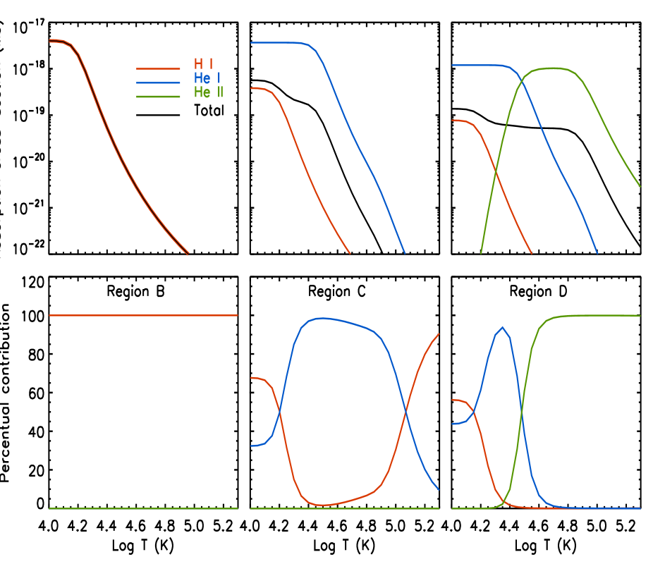
Figure 1: Top: absorption coefficient $k_{eff}$ as a function of temperature for wavelength regions B, C and D (defined in Table 1). Helium abundance has been assumed to be 5% of Hydrogen ($A_{He}=0.05$). Red: H i; Blue: He i; Green: He ii; Black: total $k_{eff}$ given by Equation 5.

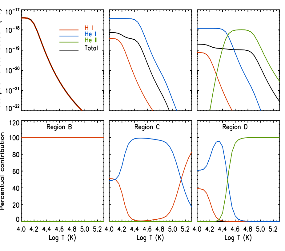
Figure 2: Same as Figure 1, with $A_{He}=0.10$.

The top panels of Figures 1 and 2 display $k_{eff}$ as a function of temperature for the B, C and D wavelength regimes, adopting the He/H values of 5% and 10%, respectively. The absorption cross sections have been calculated using the photoionization cross sections of Verner & Ferland (1996). The bottom panels show the percent contribution of each of the three ions to the total value of $k_{eff}$. In Region B absorption is only due to neutral H and as the plasma temperature rises and H ionizes, it decreases very quickly; there is no dependence on the He abundance. The temperature dependence of $k_{eff}$ is very strong for $T_{e}\geq$15,000 K, while it is very mild at lower temperatures where almost all Hydrogen is neutral.

In Regions C and D the presence of He absorption has two main effects on $k_{eff}$: first, it introduces the dependence on the He/H relative abundance; and second, it extends the range where $k_{eff}$ is weakly dependent on temperature to higher values. The latter effect is due to the fact that the ionization potential of He is larger than the H one, so that He resists ionization for a larger temperature range than H, and the fact that in region D the absorption capability lost with He i ionization is replaced by He ii absorption.

Figures 1 and 2 thus show that 1) the absorption properties of the slab depend on the electron temperature in different ways depending on the wavelength of the EUV incident radiation; and 2) they are fairly constant up to almost 100,000 K at wavelengths below 228 Å. Also, above $\approx$25,000 K the slab absorption in region D is almost exclusively due to He rather than H (in region B Hydrogen becomes again important for $T>80,000$ K), whereas they are only due to H at wavelengths between 504 Å and 912 Å.

2.2 EUV absorption as diagnostic tool

The diagnostic tool we propose in the present work capitalizes on the different temperature dependence of $k_{eff}$ in the three different wavelength regions. In order to be applied, it requires observations at wavelengths spanning at least two of the three regions; availability of observations in all three regions further increases the possible applications. Fortunately, combinations of the available space instrumentation allows the application of these technique to existing observations of both filaments (that is, prominences observed inside the solar disk) and prominences at the limb, as shown in Table 1. Almost all instruments sample wavelengths at least in two of these three ranges.

Since the temperature effects on $k_{eff}$ are most evident at temperature ranges larger than $\approx$15,000 K, this technique is best applied to prominences whose plasma is relatively hot to begin with, or is being heated, such as in erupting prominences (e.g. Landi et al. 2010).

2.3 Basic principle of the diagnostic technique

The diagnostic technique we propose relies on the determination of the extinction coefficient $e^{-\tau}$ for many different spectral lines or narrow-band filters. Let us assume for a moment that we have been able to measure the extinction coefficient $e^{-\tau}$ in Equation 1, for example by determining the ratio $F_{obs}/F_{inc}$. We will discuss in the next section a few cases where such a measurement (or an equivalent one) can be done. We will also further assume that the physical properties of the absorbing material are approximately the same along the path length $S$ of the absorbing material crossed by the line of sight. In this case, Equations 1 and 4 can be combined to give

$$\tau = k_{eff}{\left({A_{He},T}\right)}N_{H}$$ (7)

$$\ln{\left({F_{obs}/F_{inc}}\right)} = -k_{eff}{\left({A_{He},T}\right)}N_{H}$$ (8)

where $N_{H}=\int_{0}^{S}{n_{H}dl}$ is the Hydrogen column density (in cm^-2). It is important to notice that $N_{H}$ and $S$ are properties of the absorbing plasma only.

The effective absorption coefficient $k_{eff}$ can be calculated as a function of temperature for any spectral line or narrow band imaging channel, once $A_{He}$ has been specified. In case we have a narrow-band filter, $k_{eff}$ can be easily calculated as it changes slowly with wavelength over the width of the filter itself, which usually encompasses from a few to a few tens of Å (within $\approx 20$% in the available narrow-band imagers). This allows us to define and calculate as a function of temperature the function

$$L{\left({T}\right)}={{1}\over{k_{eff}{\left({T}\right)}}}\ln{\left({{{F_{obs}}\over{F_{inc}}}}\right)}={{k_{eff}{\left({T_{abs}}\right)}}\over{k_{eff}{\left({T}\right)}}}N_{H}$$ (9)

where we indicate with $T_{abs}$ the temperature of the absorbing material. The main property of the $L{\left({T}\right)}$ function is

$$L{\left({T_{abs}}\right)}=N_{H}$$ (10)

for any spectral line or narrow-band imaging channel we consider. Since $N_{H}$ is a property of the absorbing material only, the $L{\left({T_{abs}}\right)}$ values of all the spectral lines or narrow band filters are the same. Equation 10 allows us to use the function $L{\left({T_{abs}}\right)}$ in the same way as the L-function defined by Landi & Landini (1997): if we measure $F_{inc}$ and $F_{obs}$ (or some combination of them, as we will see in the next Section) for a number of spectral lines and/or narrow-band images, and plot their $L{\left({T_{abs}}\right)}$ functions in the same figure as a function of temperature, all curves will cross the same point ${\left({T_{abs},N_{H}}\right)}$. The coordinates of the crossing point can then be used to determine both the absorbing plasma electron temperature and the $N_{H}$ value; the latter can in turn be used to determine the average number density of H in the absorbing material using some assumption or estimate of the length $S$.

Also, the presence of a single crossing point for all curves provides a check on the main assumption of this technique, namely that the absorption properties of the prominence plasma are approximately the same everywhere in the prominence itself. Also, the behavior of the $L{\left({T_{abs}}\right)}$ functions of different wavelength regimes can also provide a direct determination of $A_{He}$.

2.4 Example: SDO/AIA narrow band images

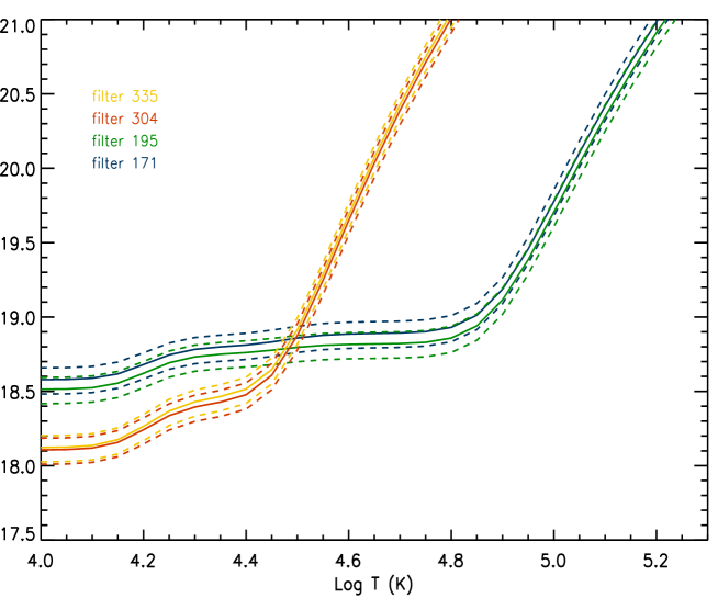
Figure 3: Example of the diagnostic technique applied to simulated intensities for four channels of the SDO/AIA narrow band imagers (see text for details). The crossing point allows to determine the plasma temperature and column density.

An example of this technique is shown in Figure 3. In this figure, simulated $F_{obs}/F_{inc}$ ratios have been calculated at the wavelengths of a few SDO/AIA channels for a prominence with total $N_{H}=6.3\times 10^{18}$ cm^-2, assuming constant $k_{eff}$ over the entire width of the filter bandbass; this corresponds to $F_{obs}/F_{inc}$ ratios of 0.66, 0.55, 0.56, and 0.49 for the 171 Å, 195 Å, 304 Å and 335 Å SDO channels, respectively. We added a small amount to the $L(T)$ functions of the 195 Å and 335 Å curves to make them more easily visible in the plot (otherwise the 304 Å and 335 Å curves, as well as the 171 Å and 195 Å curves, would have been coincident). An arbitrary 20% uncertainty has been associated to each curve and shown as dashed lines in Figure 3. The 304 Å channel has also been assumed to produce zero He ii 304 Å line emission. The He/H abundance has been assumed to be $A_{He}=0.085$. The SDO/AIA channels sample wavelengths belonging to regions $C$ and $D$, so that their $L{\left({T}\right)}$ functions have a very different temperature dependence due to the He ii absorption: as expected, their crossing point is very sharply defined and provides a rather precise measurements of $T_{abs}$ and $N_{H}$. On the contrary, channels whose wavelengths belong to the same spectral region provide completely overlapping $L{\left({T}\right)}$ functions so that they can not provide a defined crossing point. However, if their $L{\left({T}\right)}$ functions do not overlap, the difference between them can be used to indicate one (or a combination) of the following scenarios: 1) presence of emission from the absorbing material itself; 2) problems in the atomic physics; 3) possible multi-temperature structure of the absorbing prominence; 4) inaccuracy of the assumed $A_{He}$ value used to calculate $L{\left({T}\right)}$ itself.

It is important to note that when lines or channels from regions $C$ and $D$ only are available, and the temperature of the absorbing slab is between $\approx$15-20,000 K and $\simeq 80,000$ K, only He absorption is significant so that the ordinate of the crossing point allows the direct determination the Helium column density with no assumption on $A_{He}$. When lines or channels from all three wavelength ranges are available and the temperature is in the 15,000-80,000 K range, the difference in height between region $B$ $L{\left({T}\right)}$ functions and the crossing point defined by regions $C$ and $D$ $L{\left({T}\right)}$ functions provides a direct measurement of $A_{He}$. This measurement is very important in the case of erupting prominences as it can be compared with in-situ $A_{He}$ measurements from Interplanetary Coronal Mass Ejections (ICMEs).

3 Applications of the technique

In order to utilize the properties of EUV absorption for prominence plasma diagnostics, it is necessary to first define a function $L{\left({T}\right)}$ that has the properties described in the previous Section using observed EUV line or narrow-band intensities. The easiest way to achieve this is to compare intensities measured over a prominence with their values measured near the prominence itself.

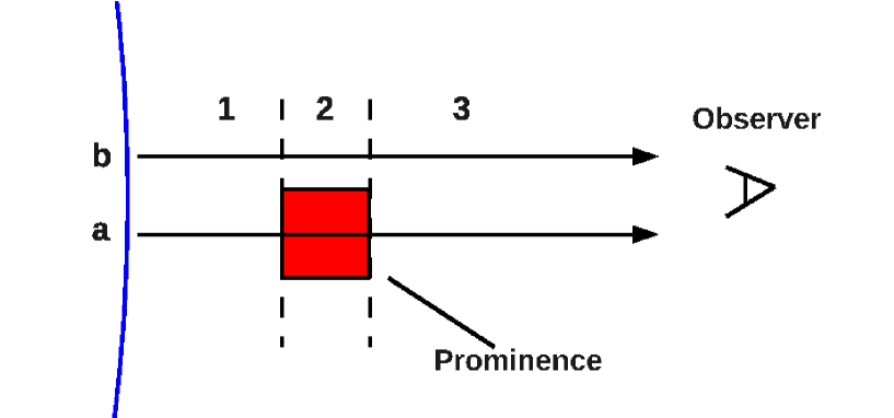
Figure 4: Cartoon showing a simplified version of the geometry discussed in Section 3. Regions 1, 2 and 3 define the “background”, “prominence” and “foreground” regions, respectively, of both lines of sight $a$ and $b$.

Figure 4 shows a simplified version of the geometry of the problem. It is the same as in Gilbert et al. (2005). Let $F_{a}$ and $F_{b}$ be the measured EUV intensity values observed along the lines of sight $a$ and $b$, where the $a$ intercepts a prominence while $b$ lies close, but outside, of it. $F_{a}$ and $F_{b}$ can be given either by spectral line intensities or narrow-band images. Both lines of sight are divided in three sections, where section 1 indicates the region below the prominence (the “background region”), section 2 corresponds to the finite length $S$ of the prominence, and section 3 covers the entire distance between the upper boundary of the prominence and the observer (the “foreground region”). The fluxes $F_{a}$ and $F_{b}$ are given by

$$F_{a} = F_{a1}e^{-\tau}+F_{a2}+F_{a3}$$

$$F_{b} = F_{b1}+F_{b2}+F_{b3}$$ (11)

Our goal is to determine $\tau$ as a function of the two observables $F_{a}$ and $F_{b}$. However, this equation has six more unknowns, namely the background, prominence and foreground intensities for each of the two line of sights, so that some assumptions are needed. First, we note that Gilbert et al. (2005) showed that the emission of the prominence itself ($F_{a2}$) at coronal temperatures is negligible. Also, when the selected lines of sight $a$ and $b$ lie close to each other, and the prominence or filament is observed far from complex plasma configurations their foreground and background emission are likely to be similar: $F_{a1}=F_{b1}=F_{1}$ and $F_{a3}=F_{b3}=F_{3}$. Thus, the set of Equations 11 simplifies to

$$F_{a} = F_{1}e^{-\tau}+F_{3}$$

$$F_{b} = F_{1}+F_{2}+F_{3}$$ (12)

where we also indicate $F_{2}=F_{b2}$ for convenience of notation.

3.1 Special case I

If the absorbing material is located at altitudes much larger than the scale height of the coronal emission in the solar atmosphere, like for example an accelerating erupting prominence during a CME onset observed against the solar disk, the emission from the foreground and from the plasma in section 2 of the line of sight becomes negligible relative to the background emission. This is due to the fact that the plasma density at or above the absorbing material height is low. In this simplified case, $F_{2}\ll F_{1}$ and $F_{3}\ll F_{1}$, so that

$$\tau = -\ln{{F_{a}}\over{F_{b}}}$$

$$L{\left({T}\right)} = -{{1}\over{k_{eff}{\left({T}\right)}}}\ln{\left({{{F_{a}}\over{F_{b}}}}\right)}$$ (13)

and the diagnostic technique outlined in the previous section can be directly applied. When time series of observations are available, this technique can provide the measurement of the erupting prominence temperature as a function of time as long as the prominence is absorbing and, if enough data are available and the plasma temperature is in the right range, also the He/H relative abundance.

3.2 Special case II

In this case we consider a quiescent prominence sitting at the solar limb in the absence of active regions in the foreground and background. Under this configuration, the foreground and background emission can be assumed to be roughly the same as their line of sight length and plasma physical conditions are approximately similar: $F_{1}\simeq F_{3}$. Also, the length of the line of sight at the limb is much larger than the prominence depth $S$, so that $F_{2}$ can be safely assumed to be negligible even if it is close to the limb. Simple algebraic considerations allow us to rewrite Equations 11 as

$$\tau = -\ln{\left({2{{F_{a}}\over{F_{b}}}-1}\right)}$$

$$L{\left({T}\right)} = -{{1}\over{k_{eff}{\left({T}\right)}}}\ln{\left({2{{F_{a}}\over{F_{b}}}-1}\right)}$$ (14)

and apply the diagnostic technique described in the previous section to the $L{\left({T}\right)}$ functions.

3.3 General case

Equations 12 have two observables and four unknown quantities, so that some assumptions (or more observables) are needed. To deal with this case, we follow the same approach as Gilbert et al. (2005). They considered a configuration where two very close parts of the prominence were observed against two very different backgrounds, and assumed that the absorption term $e^{-\tau}$ is the same in both locations. This configuration is very easily obtained when the same prominence is observed across the solar limb, so that a portion of the prominence can be studied on the disk (we will call this position $D$), and another portion lies outside the limb (position $L$).

Gilbert et al. (2005) further assumed that 1) $F_{2}$ was proportional to the foreground intensity $F_{3}$, so that $F_{2}=\gamma F_{3}$ everywhere in proximity of the prominence, and 2) that the foreground emission of the $D$ and $L$ regions have a constant ratio $F_{3}^{D}/F_{3}^{L}=\beta$. Under these assumptions, we have four different observables:

$$F_{a}^{L} = F_{1}^{L}+(\gamma+1)F_{3}^{L}$$

$$F_{b}^{L} = F_{1}^{L}e^{-\tau}+F_{3}^{L}$$ (15)

$$F_{a}^{D} = F_{1}^{D}+\beta(\gamma+1)F_{3}^{L}$$

$$F_{b}^{D} = F_{1}^{D}e^{-\tau}+\beta F_{3}^{L}$$

where $F_{a}^{D},F_{b}^{D},F_{a}^{L}$ and $F_{b}^{L}$ are observed from spectrally resolved or narrow band filter images. Simple algebraic consideration allow us to estimate the coefficient $e^{-\tau}$ as

$$e^{-\tau}={{F_{b}^{L}-\beta F_{b}^{D}}\over{F_{a}^{L}-\beta F_{a}^{D}}}$$ (16)

The advantage of Equation 16 is that it requires only the estimation of the constant $\beta$ and not of $\gamma$. Gilbert et al. (2005) determined $\beta$ assuming that the path length difference between positions $L$ and $D$ was negligible so that the only difference between the two positions was due to the intensity falloff with distance from the limb, which can be easily determined from the observations themselves.

Equation 16 can be applied to any spectral line or narrow band image for which two positions $L$ and $D$ can be selected, so that

$$\tau = -\ln{\left({{{F_{b}^{L}-\beta F_{b}^{D}}\over{F_{a}^{L}-\beta F_{a}^{D}}}}\right)}$$

$$L{\left({T}\right)} = -{{1}\over{k_{eff}{\left({T}\right)}}}\ln{\left({{{F_{b}^{L}-\beta F_{b}^{D}}\over{F_{a}^{L}-\beta F_{a}^{D}}}}\right)}$$ (17)

and the diagnostic technique can be applied.

4 Conclusions

The diagnostic technique that we have developed in this work can be very useful in several occasions. If absorption from prominence plasmas with temperature lower than $\simeq 15,000$ K is considered, the absorption coefficient does not depend on the temperature, so that the availability of lines in different spectral regions can provide an estimate of the He abundance relative to H ($A_{He}$) even without the knowledge of the thermal properties of the prominence itself.

For hotter prominences, different combinations of observations in the 3 spectral regions where absorption of different species is dominant can provide very precise temperature estimates, along with He/H and $N_{H}$ determinations. These properties are most important in studies of erupting prominences, where the prominence plasma is heated to temperatures 10 or more times typical quiescent values, and knowledge of the temporal evolution of the temperature can provide vital constraints to models of CME acceleration and heating. Also, measurements of $A_{He}$ can provide a direct, quantitative link between remote observations of erupting prominences near the Sun and in-situ measurements of the properties of prominence plasmas in the core of ICMEs.

There are two main advantages in using this method. First, the solar structures that can be studied with our technique can be easily identified and studied for long periods of time, especially when images from several channels at different wavelengths are available. Second, the diagnostic technique itself is very fast and easy to apply to large datasets, so that it allows rapid and accurate measurements of column density and plasma temperature as a function of time over extended areas. This makes this technique ideal both to study individual filaments and CME eventss, as well as to make systematic surveys on the physical properties of many events. Also, if a reasonable assumption or estimate on the geometry of the absorbing plasma can be made, this method provides a direct and relatively accurate measurement of the plasma density.

The present diagnostic technique can be applied to data from all the recent and current space missions, such as SOHO, TRACE, STEREO, Hinode and SDO, and to future ones such as Solar-C, Solar Orbiter, and Solar Probe.

Region	Wvl. range	Spectrometer	Imager
A	$\lambda>912$	SUMER
B	$504<\lambda<912$	CDS, SUMER
C	$228<\lambda<504$	CDS, EIS	EIT, EUVI, TRACE, AIA
D	$100<\lambda<228$	EIS	EIT, EUVI, TRACE, AIA

Table 1: Space-borne instruments observing EUV radiation in the four spectral regions between 100 Å and 1000 Å characterized by different H i, He i and He ii absorption properties.

References

- (1) Bryans, P., Landi, E., & Savin, D.W. 2009, ApJ, 691, 1540
- (2) Dere, K.P., Landi, E., Young, P.R., et al. 2009, A&A, 498, 915
- (3) Gilbert, H.R., Holzer, T.E., & MacQueen, R.M. 2005, ApJ, 618, 524
- (4) Gilbert, J.A., Lepri, S.T., Landi, E., & Zurbuchn, T.H. 2012, ApJ, 751, 20
- (5) Gruesbeck, J.R., Lepri, S.T., Zurbuchen, T.H., & Antiochos, S.K. 2011, ApJ, 703, 103
- (6) Gruesbeck, J.R., Lepri, S.T., & Zurbuchen, T.H. 2012, ApJ, in press
- (7) Labrosse, N., Heinzel, P., Vial, J.C., et al. 2010, Sp. Sci. Rev., 151, 243
- (8) Landi, E., & Landini, M. 1997, A&A, 327, 1230
- (9) Landi, E., Raymond, J.C., Miralles, M.P., & Hara, H. 2010, ApJ, 711, 75
- (10) Landi, E., Gruesbeck, J.R., Lepri, S.T., & Zurbuchen, T.H. 2012, ApJ, 750, 159
- (11) Lepri, S.T., & Zurbuchen, T.H. 2010, ApJ, 723, 22
- (12) Tandberg-Hanssen, 1995, The Nature of Solar Prominences, Kluwer, Dordrecht 1995
- (13) Verner, D.A., & Ferland, G.J. 1996, ApJS, 103, 467