Critical phenomena in heterogeneous $k$-core percolation

Abstract

$k$-core percolation is a percolation model which gives a notion of network functionality and has many applications in network science. In analysing the resilience of a network under random damage, an extension of this model isintroduced, allowing different vertices to have their own degree of resilience. This extension is named heterogeneous $k$-core percolation and it is characterized by several interesting critical phenomena. Here we analytically investigate binary mixtures in a wide class of configuration model networks and categorize the different critical phenomena which may occur. We observe the presence of critical and tricritical points and give a general criterion for the occurrence of a tricritical point. The calculated critical exponents show cases in which the model belongs to the same universality class of facilitated spin models studied in the context of the glass transition.

I Introduction

A significant issue in many networked infrastructures is the threat that local damage can represent to the whole system newman2003; sterbenz2010. Moreover, there is an important distinction in the way a network collapses: it can happen in a smooth, predictable way, or with extreme abruptness. The capability of designing networks where a collapse can be predicted in advance is expected to be increasingly important vespignani2010.

In recent years, there has been a wide renewal of interest in percolation models, regarding the occurrence of a first order transition, instead of the classical continuous percolation transition achlioptas2009. However, it has been also shown bizhani2012 that discontinuous transitions are not so unusual in percolation models and can be dated to severals years ago ohtsuki1987; janssen2004. Moreover, several examples have been recently proposed in the context of explosive percolation araujo2010; cho2010; chen2011; manna2011, interdependent networks parshani2010 and hierarchical lattices boettcher2012.

$k$-core percolation is an extension of percolation providing in a simple model a wide range of critical phenomena: a giant $k$-core cluster may collapse either continuously or discontinuously as a function of random damage Schonmann:1990p1812; branco1993; dorogovtsev2006. Moreover, the analysis of the $k$-core architecture of a network has developed into applications in different areas of science including protein interaction networks wuchty2005, jamming schwarz2006, neural networks Chatterjee2007, granular gases alvarez2007, evolution klimek2009, social sciences kitsak2010 and the metal-insulator transition cao2010. Finally, a set of spin model approaches to the glass transition shares close similarities with $k$-core percolation sellitto2010.

The analytical formalism of $k$-core percolation has been recently extended to include a local notion of robustness: some nodes can be more resilient than others and require a smaller number of neighbors to remain active. This extension has been named heterogeneous $k$-core (HKC) percolation and has been studied in locally tree-like networks baxter2011, finding a number of interesting critical phenomena including a tricritical point (TCP) cellai2011.

In this paper, we extend the analysis of cellai2011 to present an exhaustive description of binary mixtures in heterogeneous $k$-core percolation and show that heterogeneous $k$-core percolation models are characterized by a wealth of critical behaviors, involving both first and second order transitions. In Section 2 we define heterogeneous $k$-core percolation and explain the mathematical formalism in locally tree-like networks. In Section 3 we focus on some illustrative examples of binary mixtures of vertex types, examining the different critical phenomena and calculating relevant critical exponents. In Section 4 we give a general argument of the occurrence of a tricritical point in a binary mixtures of vertex types in heterogeneous $k$-core percolation. Finally, Section 5 states our conclusions.

II The model

Given a simple graph, a $k$-core is defined as the largest subgraph where every vertex has at least $k$ neighbors in the subgraph itself. A common way of determining the $k$-core consists in removing recursively all the vertices (and adjacent edges) with less than $k$ neighbors. We consider a framework where the nodes (and adjacent edges) of a given network are randomly removed with probability $1-p$ and we ask how the fraction of vertices in the $k$-core varies as $p$ is decreased. An analytical formalism has been developed to study this problem on the configuration model dorogovtsev2006. The configuration model is defined as the maximally random network with a given degree distribution $P(k)$. It has the important property that the number of loops vanishes as the size $N\to\infty$, which guarantees that if a $k$-core exists, it must be infinite, at least if $k\geqslant 2$ chalupa1979; dorogovtsev2006. This formalism is based on the definition of $(k-1)$-ary subtree. Given the end of an edge, a $(k-1)$-ary subtree is defined as the tree where, as we traverse it, each vertex has at least $k-1$ outgoing edges, apart from the one we came in. In configuration model networks, then, the $k$-core coincides with the $(k-1)$-ary subtree. The formalism by Dorogovtsev et al. solves the problem in any locally tree-like graphs and determines the order of the transition with which the giant $k$-core collapses dorogovtsev2006.

The heterogeneous $k$-core is an extension of the $k$-core where the minimum threshold $k_{i}$ is a local parameter, i. e. it depends on the vertex $i$. The $(k_{i}-1)$-ary subtree, then, is the tree in which, as we traverse it, each encountered vertex has at least $k_{i}-1$ child edges. We define $Z$ as the probability that a randomly chosen vertex is the root of a $(k_{i}-1)$-ary subtree and $M$ as the probability that a randomly chosen vertex is in the HKC. We can then write $M_{ab}$ for a mixture of two types of vertices $k_{a},k_{b}$ where $k_{a}$ and $k_{b}$ vertices occur with probability $r$ and $1-r$, respectively: rCl M_ab(p) &= ¯M_a(p) + ¯M_b(p)

$$\bar{M}_{a}(p)=pr\sum_{q=k_{a}}^{\infty}P(q)\sum_{l=k_{a}}^{q}\Phi_{l,q}(Z,Z)$$ (1)

$$\bar{M}_{b}(p)=p(1-r)\sum_{q=k_{b}}^{\infty}P(q)\sum_{l=k_{b}}^{q}\Phi_{l,q}(Z,Z)$$ (2)

where $\bar{M}_{a(b)}(p)$ is the fraction of nodes of type $a(b)$ in the heterogeneous $k$-core, respectively, $P(q)$ is the degree distribution of the network and we have used the convenient auxiliary function:

$$\Phi_{l,q}(X,Z)={q\choose l}(1-Z)^{q-l}\sum_{m=1}^{l}{l\choose m}X^{m}(Z-X)^{l-m}.$$

It is shown in baxter2011 that $Z$ satisfies the self-consistent equation: rCl Z &= p r ∑_q=k_a^∞ qP(q)⟨q ⟩ ∑_l=k_a-1^q-1 Φ_l,q-1(Z,Z) +
+ p(1-r)∑_q=k_b^∞ qP(q)⟨q ⟩ ∑_l=k_b-1^q-1 Φ_l,q-1(Z,Z).

In general, it is not granted that the heterogeneous $k$-core is uniquely made up of a giant cluster. As it is possible that some finite clusters of the heterogeneous $k$-core are present, Baxter et al. develop the equation for $X$, the probability that an arbitrarily chosen edge leads to a vertex which is the root of an infinite $(k_{i}-1)$-ary subtree. In the case of a binary mixture, the equation reads rCl X &= pr ∑_q=k_a^∞ qP(q)⟨q ⟩ ∑_l=k_a-1^q-1 Φ_l,q-1(X,Z) +
+p(1-r)∑_q=k_b^∞ qP(q)⟨q ⟩ ∑_l=k_b-1^q-1 Φ_l,q-1(X,Z),

Therefore, the probability $\mathcal{S}_{ab}$ that a randomly chosen vertex belongs to the giant HKC is

$$\mathcal{S}_{ab}=\sum_{l\geq k_{a}}\mathcal{S}_{a}(l)+\sum_{l\geq k_{b}}\mathcal{S}_{b}(l)$$ (3)

with

$$\mathcal{S}_{a}(l)=pr\sum_{q\geq l}P(q)\Phi_{l,q}(X,Z),$$ (4)

$$\mathcal{S}_{b}(l)=p(1-r)\sum_{q\geq l}P(q)\Phi_{l,q}(X,Z).$$ (5)

$\mathcal{S}_{a(b)}(l)$, then, is the probability that an $a(b)-$vertex in the giant HKC has exactly $l\geq k_{a(b)}$ neighbors in the giant HKC, respectively. Those expressions are analogous to (1) and (2), as can be seen after using the identity $\sum_{q=k}^{\infty}\sum_{l=k}^{q}c_{q,l}=\sum_{l=k}^{\infty}\sum_{q=l}^{\infty}c_{q,l}$, valid for any function $c_{q,l}$.

An important concept in $k$-core percolation is the corona. The corona is defined as the subset of the HKC where every vertex $i$ has exactly $k_{i}$ nearest neighbours in the HKC. By definition, then, a corona cluster is characterized by the property that if only one of its vertices is removed, the whole cluster collapses. It can be shown that the corona clusters are finite everywhere except at the phase transition, where the mean cluster size diverges goltsev2006; baxter2011. Using equation (3), then, the corona $\mathcal{C}_{ab}$ of a binary mixture is given by the following formula

$$\mathcal{C}_{ab} = \mathcal{S}_{a}(k_{a})+\mathcal{S}_{b}(k_{b})=$$ (6)

$$= pr\sum_{q\geq k_{a}}P(q)\Phi_{k_{a},q}(X,Z)+$$

$$+p(1-r)\sum_{q\geq k_{b}}P(q)\Phi_{k_{b},q}(X,Z).$$

The distinction between heterogeneous $k$-core clusters and the giant heterogeneous $k$-core has to be made whenever the two do not coincide. That is the case when we consider binary mixtures of the type $k_{a}=1$, $k_{b}>1$, as for $k=1$ finite 1-core clusters are possible. However, for mixtures such as $2\leq k_{a}<k_{b}$, no finite heterogeneous $k$-cores are possible, therefore: $X=Z$ and $M_{ab}=\mathcal{S}_{ab}$.

As in the homogeneous case, also in heterogeneous $k$-core percolation a $k$-core architecture of the network can be defined. Therefore we define a heterogeneous sub-core as a subset of the HKC where a higher threshold $k_{i}$ is imposed on some or all vertex types. More specifically, given a HKC of type $k_{a}$, $k_{b}$, the strength $M_{k}$ of a heterogeneous sub-core is given by

$$M_{k} = pr\sum_{l\geq h_{a}}\sum_{q\geq l}P(q)\Phi_{l,q}(Z,Z)+$$ (7)

$$+p(1-r)\sum_{l\geq h_{b}}\sum_{q\geq l}P(q)\Phi_{l,q}(Z,Z),$$

where $h_{a}=max(k,k_{a})$ and $h_{b}=max(k,k_{b})$. An analogous expression holds for $\mathcal{S}_{k}$:

$$\mathcal{S}_{k} = pr\sum_{l\geq h_{a}}\sum_{q\geq l}P(q)\Phi_{l,q}(X,Z)+$$ (8)

$$+p(1-r)\sum_{l\geq h_{b}}\sum_{q\geq l}P(q)\Phi_{l,q}(X,Z).$$

Therefore, when considering for example a binary HKC with $k_{a}<k_{b}$, sub-cores with $k\leq k_{a}$ coincide with the HKC, whereas sub-cores with $k>k_{a}$ are proper subsets of the HKC.

III Illustrative examples

We consider now a few examples of binary mixtures on Erdős-Rényi graphs with the most interesting critical phenomena. Plugging in the Poissonian degree distribution $P(q)=z_{1}^{q}\exp(-z_{1})/q!$ (where $z_{1}$ is the mean degree) into equations (II) and (II), the sums can be calculated analytically and several critical phenomena can be found. First, we review two cases already studied in the literature: the case $\mathbf{k}=(k_{a},k_{b})=(1,3)$, examined in baxter2011 on the Bethe lattice, and the case $\mathbf{k}=(2,3)$ cellai2011. Then, we focus on the case $\mathbf{k}=(2,4)$, and show that its phase diagram is qualitatively identical to the ones of the type $k_{a}=1$, $k_{b}\geq 3$, and represents a quite general behavior, with applications to the theory of glass transitions.

III.1 The case $k_{a}=1$, $k_{b}=3$

In this case we have to take into consideration that, due to the presence of vertices of type 1, there are finite $k$-cores. The two equations (II) and (II) can be re-written as

$$pf_{13}(Z) = 1$$ (9)

$$ph_{13}(X,Z) = 1,$$ (10)

where

$$f_{13}(Z)=\frac{1-(1-r)e^{-z_{1}Z}(1+z_{1}Z)}{Z},$$ (11)

$$h_{13}(X,Z)=\frac{1-e^{-z_{1}X}}{X}-(1-r)z_{1}e^{-z_{1}Z}.$$ (12)

It can be shown that the locus defined by $f_{13}^{\prime}(Z)=0$ corresponds to a line of first order transitions which ends into a critical point defined by $f_{13}^{\prime}(Z)=f_{13}^{\prime\prime}(Z)=0$ . A simple calculation yields:

$$r_{c}=1-\frac{1}{3}e$$ (13)

$$p_{c}=\frac{3}{z_{1}}$$ (14)

$$Z_{c}=\frac{1}{z_{1}}$$ (15)

$X_{c}$ has no analytic expression, being the non-trivial solution of the equation $1-\exp(-z_{1}X_{c})=2/3z_{1}X_{c}$, which is $z_{1}X_{c}\simeq 0.874$.

Using (3), we can calculate the strength of the giant HKC as

$$\mathcal{S}_{13} = p\left[1-e^{-z_{1}X}\right]+$$ (16)

$$-p(1-r)z_{1}Xe^{-z_{1}Z}\left(1+z_{1}Z-\frac{1}{2}z_{1}X\right),$$

and we can also derive the expression of the 2-sub-core (from eq. (8)):

$$\mathcal{S}_{2} = pr(1-e^{-z_{1}X}-z_{1}Xe^{-z_{1}Z})+$$ (17)

$$+p(1-r)\left[1-e^{-z_{1}X}+\right.$$

$$\left.-z_{1}Xe^{-z_{1}Z}\left(1+z_{1}Z-\frac{1}{2}z_{1}X\right)\right].$$

Using (6), the strength of the HKC corona is given by the following expression:

$$\mathcal{C}_{13} = pe^{-z_{1}Z}\left[rz_{1}X+\right.$$ (18)

$$\left.+\frac{1}{6}(1-r)z_{1}^{3}\left(3Z^{2}X-3ZX^{2}+X^{3}\right)\right].$$

In particular, the fraction of vertices of each type in the HKC are given by the following expressions:

$$\bar{\mathcal{S}}_{1}=pr(1-e^{-z_{1}X})$$ (19)

$$\bar{\mathcal{S}}_{3}=p(1-r)\left[1-e^{-z_{1}X}-z_{1}Xe^{-z_{1}Z}\left(1+z_{1}Z-\frac{1}{2}z_{1}X\right)\right]$$ (20)

The critical percolating strengths can be calculated with arbitrary precision. The approximate values are given in Table I.

$r_{c}$	$z_{1}\mathcal{S}^{c}_{13}$	$z_{1}\mathcal{C}^{c}_{13}$	$z_{1}\bar{\mathcal{S}}^{c}_{1}$	$z_{1}\bar{\mathcal{S}}^{c}_{3}$
0.0939	0.3821	0.2700	0.1642	0.2179

Table 1: Critical fractions of some relevant quantities in the case $\mathbf{k}=(1,3)$.

Figure 1 displays the phase diagram of the mixture $\mathbf{k}=(1,3)$ for a Erdős-Rényi graph. The two phase region occurs at a relatively low value of $r_{c}$, meaning that many 3-nodes are necessary to drive the system towards the first order (hybrid) transition. The relative composition of the giant HKC, instead, presents a much higher fraction of 1-nodes, due to the high fragility of 3-nodes with respect to 1-nodes. The phase diagram also shows that the corona strength is much smaller than $\mathcal{S}_{13}$ on the right side of the coexistence region, whereas is much closer to $\mathcal{S}_{13}$ on the left side, showing that the corona clusters dominate the HKC in the 1-rich phase.

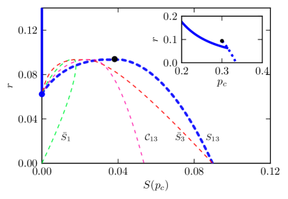
Figure 1: Phase diagram of the case $\mathbf{k}=(1,3)$ for the Erdős-Rényi graph ($z_{1}=10$). The main panel illustrates the critical values of the giant HKC strength. The blue lines report the second order (solid) and the first order (dashed) transitions. The critical (black) and the critical end point (blue) are indicated by a dot. The fractions of nodes of type 1 ($\bar{\mathcal{S}}_{1}$) and 3 ($\bar{\mathcal{S}}_{3}$) in the giant HKC are also reported. The corona size $\mathcal{C}_{13}$ is represented by a magenta dashed line. The inset reports the most relevant detail of the phase diagram in the space ($r$,$p_{c}$).

III.2 The case $k_{a}=2$, $k_{b}=3$

As shown in our recent paper, this case has the property $X=Z$ and is characterized by a tricritical point cellai2011. We review the peculiarities of this case. The quantity $Z$ at a given damage fraction $(1-p)$ can be calculated by solving the equation $pf_{23}(Z)=1$, where

$$f_{23}(Z)=\frac{1-e^{-z_{1}Z}[1+(1-r)z_{1}Z]}{Z}.$$ (21)

From (II), the strength of the heterogeneous $k$-core is given by

$$M_{23}(p)=p\left\{1-e^{-z_{1}Z}\left[1+z_{1}Z+\frac{1}{2}(1-r)z_{1}^{2}Z^{2}\right]\right\}.$$ (22)

It is easy to see that $f_{23}(Z)$ has a maximum at a finite $Z$ for $r<1/2$, which continuously moves to $Z=0$ at exactly $r=1/2$. This implies that there is a line of first order transitions for $r<1/2$, and a second order percolating transition for $r>1/2$. At $r=1/2$, the two lines match exactly at a tricritical point (TCP). The critical exponent $\beta$ at the transition $M_{23}(p)-M_{23}(p_{c})\sim(p-p_{c})^{\beta}$, can be calculated analytically:

$$\beta=\left\{\begin{array}[]{lcrcl}2&&1/2\leqslant&r&<1\\ 1&&&r&=1/2\\ 1/2&&0\leqslant&r&<1/2\end{array}\right.$$ (23)

The value of the exponent $\beta$ at $r<1/2$ agrees with the typical hybrid transition phenomenology dorogovtsev2006; branco1993, whereas for $r>1/2$ we recover the exponent of classical percolation without dangling ends Schonmann:1990p1812. The value of $\beta$ at the TCP does not change when it is calculated along a line at fixed $p_{c}$.

Another exponent which can be calculated analytically is the one which governs the vanishing of the coexistence region as $r\to 1/2^{-}$. We indicate it as $M^{*}(r)\sim\left(\frac{1}{2}-r\right)^{\beta_{u}}$, with $\beta_{u}=2$. Finally, the rotation defining the critical fields is

$$\left(\begin{array}[]{c}\mu_{\perp}\\ \mu_{\parallel}\end{array}\right)=\left(\begin{array}[]{cc}\cos\theta&\sin\theta\\ -\sin\theta&\cos\theta\\ \end{array}\right)\left(\begin{array}[]{c}p-p_{t}\\ r-r_{t}\end{array}\right)$$ (24)

with $\tan\theta=4/z_{1}$. Close to the tricritical point, the critical line has a behavior $\mu_{\parallel}\sim\mu_{\perp}^{1/2}$, with a crossover exponent $\varphi_{t}=2$.

Fig. 2 shows the phase diagram of this case. The system undergoes a first order (hybrid) phase transition for $r<1/2$, which smoothly shrinks at the TCP. The fractions $\bar{M}_{2}$ and $\bar{M}_{3}$ of nodes of each type inside the HKC are also plotted. It is interesting to note that $\bar{M}_{2}$ is substantially higher than $\bar{M}_{3}$ in the proximity of the TCP. This behavior, which is the opposite of what occurs in the case $\mathbf{k}=(1,3)$, appears to be related to the higher value of $r$ at which the TCP occurs: the fraction of nodes of type 2 in the critical HKC steadily grows along the first order line as the coexistence region shrinks. In the case $\mathbf{k}=(1,3)$, instead, the critical point occurs at quite a low $r$, due to the high stability of type 1 nodes, before the switch between the two mixture components. It appears that the vanishing of the discontinuity is finely tuned by the vanishing fraction of type 3 nodes in the HKC. At the same time, of course, the fraction of type 2 nodes becomes increasingly important, determining the change of order of the transition at the TCP.

\begin{overpic}[width=216.81pt]{plot_phase_mass_23_pub} \put(59.0,27.0){\includegraphics[height=86.72267pt,angle={0},keepaspectratio={true}]{plot_phase_pc_23} } \end{overpic}

Figure 2: Phase diagram of the $\mathbf{k}=(2,3)$ mixture, showing the total mass of the percolating heterogeneous $k$-core cluster at different compositions $r$, for Erdős-Rényi networks with $z_{1}=10$. The TCP at $r=1/2$ separates a line of first order transitions (dashed) from the second order line (solid). The masses of the fractions of nodes of types 2 (green) and 3 (red) in the giant HKC are also shown. The inset shows the phase diagram in the $(r,p)$ space.

III.3 The case $k_{a}=2$, $k_{b}=4$

From equation (II), the case $k_{a}=2$, $k_{b}=4$ is solved by $pf_{24}(Z)=1$, where

$$f_{24}(Z)=\frac{1-e^{-z_{1}Z}\left\{1+(1-r)\left(z_{1}Z+\frac{1}{2}z_{1}^{2}Z^{2}\right)\right\}}{Z}.$$ (25)

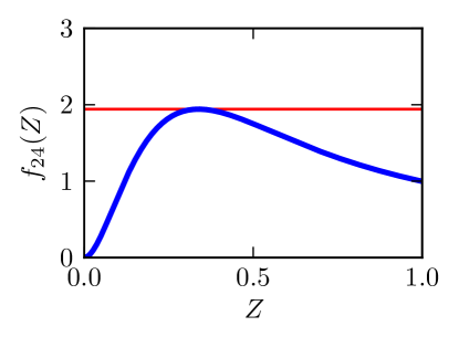
(a) $r=0$

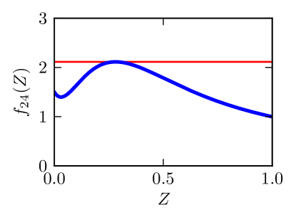
(b) $r=0.15$

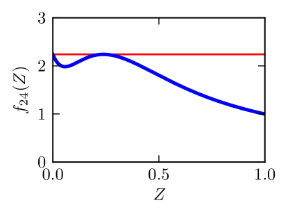
(c) $r=r_{cep}$

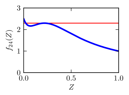
(d) $r=0.25$

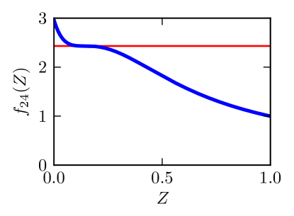
(e) $r=r_{c}$

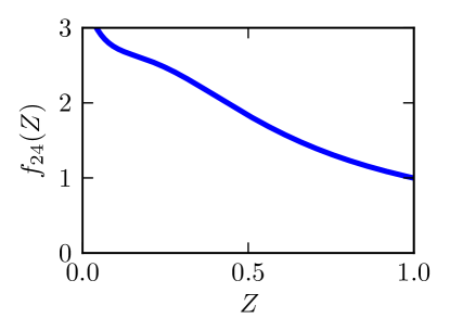
(f) $r=0.35$

Figure 3: Different scenarios of the solutions of equation $pf_{24}(Z)=1$ in the case $k_{a}=2$, $k_{b}=4$ for different values of $r$ ($z_{1}=10$). The red horizontal line marks the value of $1/p_{c}$ where the first order transition occurs. In the panels (a) and (b) there is a first order transition corresponding to the global maximum of $f_{24}(Z)$; in (c) the maximum is at the same height as $f_{24}(Z=0)$ (critical end point); in (d) there is both a first and a second order transition; in (e) the first order transition disappears into a critical point; in (f) only the classical percolation transition at $Z=0$ remains.

Differently from the case $k_{a}=2$, $k_{b}=3$, here for some values of $r$ the function $f_{24}$ has a local maximum which does not approach the $Z=0$ point. More specifically, it is easy to show that $f_{24}(Z)$ has three types of behavior: monotonously decreasing, a local maximum at $Z>0$, and a global maximum at $Z>0$ (Fig. 3). A global maximum at $Z=0$ corresponds to a second order de-percolating transition, as the solution of equation $pf_{24}(Z)=1$ smoothly vanishes at some $p_{c}$. A local maximum at $Z>0$, instead, determines a first order transition line between two stable giant HKCs.

Using equation (II), the strength of the HKC can be re-written as

$$M_{24}(p) = p\left\{1-e^{-z_{1}Z}\left[1+z_{1}Z+\frac{1}{2}(1-r)z_{1}^{2}Z^{2}+\right.\right.$$ (26)

$$+\left.\left.\frac{1}{6}(1-r)z_{1}^{3}Z^{3}\right]\right\}.$$

From the definition (7), the strength of the heterogeneous sub-core as a subset of the HKC is given by

$$M_{k}(p)=\mathcal{M}^{a}_{k}+\mathcal{M}^{b}_{k},$$ (27)

where

$$\mathcal{M}^{a}_{k}=pr\left[1-e^{-z_{1}Z}\sum_{n=0}^{h_{a}-1}\frac{(z_{1}Z)^{n}}{n!}\right]$$ (28)

$$\mathcal{M}^{b}_{k}=p(1-r)\left[1-e^{-z_{1}Z}\sum_{n=0}^{h_{b}-1}\frac{(z_{1}Z)^{n}}{n!}\right]$$ (29)

and $h_{a(b)}=max(k,k_{a(b)})$. For $k\leq 2$, the sub-core coincides with the HKC and for instance we have $M_{2}=M_{24}$. For $k\geq 4$, the sub-core is a proper subset of the HKC, but the vertex distinction is not longer relevant, as the threshold $k$ applies in the same way to both vertex types. Therefore, the sub-core coincides with the usual homogeneous $k$-core. The most interesting case is when $k=3$, as this threshold restricts the number of acceptable type 4 vertices, but it has no effect on the threshold of type 2 vertices. We indicate the corresponding strength as $M_{3}$, which is given by the following formula from (27):

$$M_{3}(p) = p\left\{1-e^{-z_{1}Z}\left[1+z_{1}Z+\frac{1}{2}z_{1}^{2}Z^{2}\right.\right.+$$ (30)

$$+\left.\left.\frac{1}{6}(1-r)z_{1}^{3}Z^{3}\right]\right\}.$$

From (25), we calculate the phase diagram at different compositions $r$ (Fig. 4). At high $r$, the phase diagram is characterized by a critical line of de-percolating transitions. This line meets a first order line at a point which is usually called a critical end point in condensed matter physics. The first order line corresponds to the type of hybrid transition observed in $k$-core percolation for $k\geq 3$. Differently from the case $k_{a}=2$, $k_{b}=3$, here the first order line presents a critical point at the end of a two-phase coexistence between a low and a high density phase.

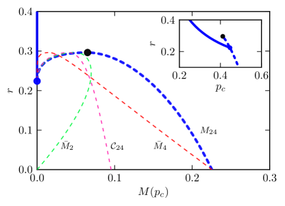
Figure 4: Phase diagram of the case $\mathbf{k}=(2,4)$ for the Erdős-Rényi graph ($z_{1}=10$) in the space ($r$,$M$), main panel, and ($r$,$p$), inset. Symbols are as in Fig. 1

.

The position of the critical end point is determined by imposing $f_{24}^{\prime}(Z)=0$ and $f_{24}(Z)=rz_{1}$, which yield the solution $r_{cep}=0.2239964831566\dots$. Now we consider the strength $M_{24}^{*}(r)$ of the HKC along the low density border of the coexistence region in approaching the critical end point. We define the critical exponent $\beta_{cep}$ of the critical end point from the manner in which such low density border vanishes: $M_{24}^{*}(r)\sim(r-r_{cep})^{\beta_{cep}}$. It emerges that as $r\to r_{cep}^{+}$ we have:

$$M_{24}^{*}(r)\sim(r-r_{cep})^{2},$$ (31)

which implies that $\beta_{cep}=2$. The strength of the $3$-sub-core in the HKC can be calculated in a similar way

$$M_{3}^{*}(r)\sim(r-r_{cep})^{3}.$$ (32)

The higher exponent of $M_{3}^{*}$ with respect to $M_{24}^{*}$ implies that the critical 2-nodes are essential for observing the critical end point. The $k=3$ threshold, in fact, recursively eliminates all the type 2 nodes with exactly two neighbors, triggering a cascade which essentially makes the sub-core become a negligible fraction of the HKC.

The critical point can be calculated by requiring that the maximum ($f_{24}^{\prime}(Z)=0$) coincides with the second change in convexity ($f_{24}^{\prime\prime}(Z)=0$). Hence we get an equation for the critical composition $r_{c}$:

$$\exp\left(1+\sqrt{\frac{1-3r_{c}}{1-r_{c}}}\right)=5-7r_{c}+4\sqrt{(1-r_{c})(1-3r_{c})},$$ (33)

with numerical solution $r_{c}\approx 0.2962590188$. Using the appropriate equations we can calculate with arbitrary precision the critical damage $p_{c}$ and the values of the $k$-core strengths: they are summarized in Table II.

$r_{c}$	$z_{1}p_{c}$	$z_{1}M^{c}_{24}$	$z_{1}C^{c}_{24}$	$z_{1}\bar{M}^{c}_{2}$	$z_{1}\bar{M}^{c}_{4}$	$z_{1}M^{c}_{3}$
0.2963	4.1131	0.6510	0.4079	0.4963	0.1547	0.3569

Table 2: Critical fractions of some relevant quantities in the case $\mathbf{k}=(2,4)$.

The critical exponent $\beta$ defined by $M_{24}(p)-M_{24}(p_{c})\sim(p-p_{c})^{\beta}$ can be calculated analytically for each region of the phase diagram:

$$\beta=\left\{\begin{array}[]{lll}2&\textrm{critical line}&r>r_{cep}\\ 1/2&\textrm{hybrid transition}&r<r_{c}\\ 1/3&\textrm{hybrid transition}&r=r_{c}\end{array}\right.$$ (34)

In the region $r_{cep}<r<r_{c}$, the first order transition separates two percolating phases and therefore it is possible to calculate the exponent $\beta^{\prime}$ on the left hand side of the first order line (Fig. 4):

$$\beta^{\prime}=\left\{\begin{array}[]{ll}1&r_{cep}<r<r_{c}\\ 1/3&r=r_{c}\end{array}\right.$$ (35)

The exponent $\beta^{\prime}=1$ away from the critical point is not singular, whereas from the other side of the first order transition it is $\beta=1/2$. This difference is due to the presence of the hybrid transition, which is asymmetric. However, the two exponents coincide at the critical point as generally expected.

It is interesting to note that the exponents at the hybrid transition in (34) exactly match the ones found in facilitated spin models reproducing mode-coupling theory singularities sellitto2012. In particular, exponent $1/2$ corresponds to the $A_{2}$ singularity associated to a discontinuous liquid-glass transition, whereas the exponent $1/3$ corresponds to the $A_{3}$ singularity at the endpoint of the discontinuous glass-glass transition of the $F_{13}$ schematic model sellitto2012; goetze2009.

The difference $\Delta M_{24}$ of the two coexisting HKC strengths as $r\to r_{c}^{-}$ vanishes according to the following law:

$$\Delta M_{24}\sim(r_{c}-r)^{1/2}.$$ (36)

Therefore, the associated critical exponent is $\beta_{u}=1/2$. The expansion of $\Delta M_{3}$ yields the same critical exponent

$$\Delta M_{3}\sim(r_{c}-r)^{1/2}.$$ (37)

The phase diagram, then, is characterized by the same topology as in the $k_{a}=1$, $k_{b}=3$ case: a first order (hybrid) transition line which ends in a critical point and a critical line which encounters the first order line at a critical end point. Here the critical point occurs at a higher fraction of low-$k$ nodes, and at a larger fraction of low $k$ nodes in the composition of the HKC: the opposite of the case $\mathbf{k}=(1,3)$. This is presumably due to the higher fragility of 4-nodes with respect to 3-nodes.

III.4 The case $k_{a}=3$, $k_{b}=8$

Binary mixtures involving thresholds higher than 2 cannot present continuous transitions. However, the mixing of different types of nodes may still result in a critical point. Fig. 5 shows the phase diagram of the case $\mathbf{k}=(3,8)$ as an example of this behavior. The high difference in resilience between 3-nodes and 8-nodes results in an intermediate region of the phase diagram where an 8-rich phase collapses into a 3-rich phase. The two lines of first order transitions do not match smoothly, and a region with a stable 3-rich percolating phase can be easily seen. It can be shown that the critical point is in the same universality class as the one in the case $\mathbf{k}=(2,4)$, with the same critical exponents along the first order line.

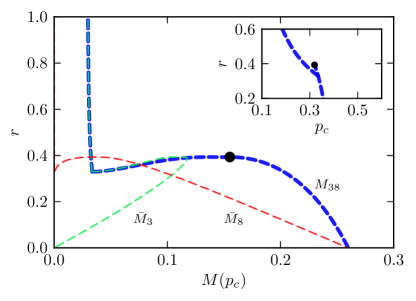
Figure 5: Phase diagram of the case $\mathbf{k}=(3,8)$ for the Erdős-Rényi graph ($z_{1}=30$). Symbols are as in Fig. 1. Differently from the previous cases, here there are two lines of first order transitions and no classical continuous percolation scenario.

III.5 Summary

Fig. 6 summarizes the phase diagram of a few relevant binary mixtures. The general behavior of mixtures of type $\mathbf{k}=(1,k)$ or $\mathbf{k}=(2,k)$ is characterized by a critical line and a line of first order transitions which ends in a critical point. The case $\mathbf{k}=(2,3)$, however, is quite peculiar as the two lines match at a tricritical point. This occurrence is not obvious and will be investigated in the next section. Both the tricritical and the critical point observed in most mixtures belong to the same universality class of facilitated spin models reproducing mode coupling theory singularities of type $F_{12}$ and $F_{13}$, respectively sellitto2012; arenzon2012.

Fig. 6 also reports the case $\mathbf{k}=(3,4)$ as an example where there cannot be continuous transitions, as both values of $k$ are larger than 2. The mixture $\mathbf{k}=(3,4)$ is only characterized by a line of first order transitions. As we have seen in the case $k=(3,8)$, though, a critical point can still arise when the two values of $k$ are quite far from each other so that the high-$k$ phase can collapse without undermining the stability of a low-$k$ phase (Fig. 5).

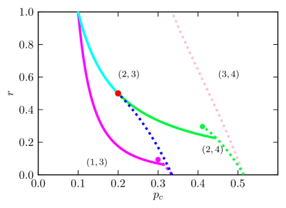
Figure 6: Comparison of the phase diagrams of the cases $\mathbf{k}=(1,3)$, $\mathbf{k}=(2,3)$, $\mathbf{k}=(2,4)$ and $\mathbf{k}=(3,4)$ for Erdős-Rényi graphs with $z_{1}=10$. As in the previous phase diagrams, continuous lines represent continuous phase transitions, whereas dashed lines represent first order phase transitions. The red dot represents a TCP; the other dots are critical points.

IV A criterion for a tricritical point

We have already noted that the occurrence of a TCP is quite peculiar in this type of models, but quite resilient to different network topologies cellai2011. In this section we give some insight into the origin of a TCP and show a criterion to establish the occurrence of it in a given binary mixture of vertices. As a general rule, given a binary mixture $\mathbf{k}=(k_{a},k_{b})$ where $k_{a}$- and $k_{b}$-cores are characterized by a second and a first order transition, respectively, the TCP occurs whenever the critical point associated with to the discontinuous transition of the $k_{b}$-rich mixture coincides with a vanishing HKC strength. The critical percolation line, by definition, is characterized by a vanishing HKC and must match the first order line to give origin to a TCP.

In the following we assume that the degree distribution $P(q)$ satisfies

$$0<\sum_{q=3}^{+\infty}q(q-1)(q-2)P(q)<+\infty.$$ (38)

This condition is quite general, as it has already been shown that scale free networks with $P(q)\sim q^{-\gamma}$ (for large $q$) and $1<\gamma\leq 3$ are not characterized by first order transitions and therefore their phase diagrams cannot involve neither critical or tricritical points dorogovtsev2006. Therefore, the only interesting case where the following analysis does not apply involves scale free networks with $3<\gamma\leq 4$.

Due to the different properties of binary mixtures, we differentiate two cases according to the presence of finite HKC clusters or not.

IV.1 The case $k_{a}=2$, $k_{b}=k\geq 3$

In the case $\mathbf{k}=(2,k)$, equation (II) can be re-written as $pf_{2k}(Z)=1$, where the relevant function is rCl f_2k(Z) &= r∑_q=2^+∞ qP(q)⟨q ⟩ ∑_l=1^q-1 (q-1 l) Z^l-1(1-Z)^q-1-l +
+(1-r)∑_q=k^+∞ qP(q)⟨q ⟩ ∑_l=k-1^q-1 (q-1 l) Z^l-1(1-Z)^q-1-l.
In this case $X=Z$, so we only need to study the behaviour of the equation at $Z\to 0^{+}$. The expansion reads rCl f_2k(Z) &= r∑_q=2^+∞ q(q-1)P(q)⟨q ⟩ +
-12r ∑_q=2^+∞ q(q-1)(q-2)P(q)⟨q ⟩Z +O(Z^2) +
+(1-r)∑_q=k^+∞ qP(q)⟨q ⟩ (q-1 k-1) Z^k-2 + O(Z^k-1).
A necessary condition for a critical point which continuously approaches the line $Z=0$ for $r\to r_{c}$ is that $f_{2k}^{\prime}(0)=0$ at $r=r_{c}$. From equation (IV.1), we have two possibilities. If $k\geq 4$,

$$f_{2k}^{\prime}(0)=-\frac{1}{2}r\sum_{q=2}^{+\infty}\frac{q(q-1)(q-2)P(q)}{\langle q\rangle},$$ (39)

which is always negative and vanishes only for $r=0$. If $k=3$, instead, the linear term proportional to $r$ mixes with the linear term from the type 3 nodes and we get

$$f_{23}^{\prime}(0)=\left(\frac{1}{2}-r\right)\sum_{q=3}^{+\infty}\frac{q(q-1)(q-2)P(q)}{\langle q\rangle},$$ (40)

which vanishes at $r=1/2$.

From equation (IV.1) it transpires that $Zf_{2k}(Z)$ can be written as an expansion in terms of core shells for each node type. The condition of the critical point $f_{2k}^{\prime}(Z)=0$ implies that the dominant term for $Z\to 0^{+}$ is the linear one. The term $r\sum_{q}\frac{q(q-1)(q-2)P(q)}{2\langle q\rangle}Z^{2}$ represents the probability that, following an edge leading to a node of type 2, there are two outgoing edges connected to the HKC (i. e. there must be exactly one extra neighbor beyond the minimum possible). The term $(1-r)\sum_{q}\frac{qP(q)}{\langle q\rangle}{q-1\choose k-1}Z^{k-1}$ represents the probability that, following an edge leading to a node of type $k$, there are $k-1$ outgoing edges connected to the HKC. In other words, this is the probability that the $k$-node found at the end of the edge is connected to the $k$-corona. The condition for a TCP, therefore, is that the $3$-shell term of the type 2 nodes has the same order of magnitude as the $k$-corona of the $k$ type nodes. This can only occur when $k=3$, where we have a TCP at $r=1/2$ (see also Eq. 40).

IV.2 The case $k_{a}=1$, $k_{b}=k\geq 3$

As noticed in Section 3, finite $k$-cores exist when $k=1$ cellai2011. Therefore, we have $X<Z$, and the functions associated to the two relevant equations (II) and (II) are:

$$f_{1k}(Z)=\frac{r}{Z}+(1-r)\sum_{q=k}^{+\infty}\frac{qP(q)}{\langle q\rangle}\sum_{l=k-1}^{q-1}{q-1\choose l}Z^{l-1}(1-Z)^{q-1-l},$$ (41)

rCl h_1k(X,Z) &= r ∑_q=0^+∞ q P(q)⟨q ⟩ ∑_m=1^q-1 (q-1 m) X^m-1 (1-X)^q-1-m+
+(1-r)∑_q=k^+∞ qP(q)⟨q ⟩ ∑_l=k-1^q-1 (q-1 l) (1-Z)^q-1-l ×
×∑_m=1^l (l m) X^m-1 (Z-X)^l-m. As in the case $\mathbf{k}=(2,k)$, it is meaningful to expand $h(X,Z)$ for $X\to 0^{+}$:

$$h_{1k}(X,Z)=a_{0}(Z)+a_{1}(Z)X+O(X^{2}),$$ (42)

where rCl a_0(Z) &= r∑_q=2^+∞ q(q-1)P(q)⟨q ⟩ +(1-r) ∑_q=k^+∞qP(q)⟨q ⟩ ×
×∑_l=k-1^q-1 (q-1 l)l Z^l-1(1-Z)^q-1-l; rCl a_1(Z) &= -12r ∑_q=2^+∞ q(q-1)(q-2)P(q)⟨q ⟩ +
-12(1-r) ∑_q=k^+∞ qP(q)⟨q ⟩∑_l=k-1^q-1 (q-1 l)×
×l (l-1) Z^l-2(1-Z)^q-1-l. It is important to remark that $a_{1}(Z)<0$ for every $Z$, i. e. $h(0,Z)$ is always a local maximum of $h$ as a function of $X$.

If a TCP exists, there must exist a value of $r$ for which a critical point (the endpoint of a line of first order transitions) occurs exactly at $X=0$, as this corresponds to the critical line. As $\lim_{Z\to 0}f_{1k}(Z)=+\infty$ for every $r>0$ (Eq. 41), the equation $pf_{1k}(Z)=1$ never has a solution $Z=0$ and $f_{1k}$ is monotonic in the neighborhood of $Z=0$. Therefore, a line of first order transitions corresponds to a local maximum of $f_{1k}$, where equation $pf_{1k}(Z)=1$ has two solutions. The discontinuity in the solution $Z(p)$ provokes a discontinuity in the solution $X(p)$ of the second equation. This in turn causes a discontinuity in the strength $\mathcal{S}$ of the giant HKC. Therefore, if a critical point occurs at $Z=Z_{c}$, it must be $f_{1k}^{\prime}(Z_{c})=f_{1k}^{\prime\prime}(Z_{c})=0$. (The local maximum of $f$ cannot occur at $Z=0$, as we have seen.) In order to have a TCP, the above defined critical point must occur at $X_{c}=0$. This implies that the fraction $p_{c}$ of undamaged nodes at criticality must satisfy the inequality

$$h_{1k}(0,Z_{c})\leq\frac{1}{p_{c}}.$$ (43)

Using the first equation, this is equivalent to

$$h_{1k}(0,Z_{c})\leq f(Z_{c}),$$ (44)

where $f_{1k}^{\prime}(Z_{c})=f_{1k}^{\prime\prime}(Z_{c})=0$ and, in case of multiple solutions, the value of $Z_{c}$ where $f_{1k}(Z_{c})$ is highest must be considered.

The condition (44) is only a necessary condition for a TCP, because in general it may be possible that $h$ has a maximum higher than $h_{1k}(0,Z)$. However, we now show that this condition is violated for all values of $k$. Let us consider the two conditions:

$$\begin{cases}h_{1k}(0,Z)\leq f_{1k}(Z)\\ f_{1k}^{\prime}(Z)=0\end{cases}.$$ (45)

Substituting the second equation into the first one yields rCl $\displaystyle r\sum_{q=2}^{+\infty}\frac{q(q-1)P(q)}{\langle q\rangle}Z+$
&+ (1-r) ∑_q=k^+∞ qP(q)⟨q ⟩ ∑