address=Racah Institute of Physics, The Hebrew University, Jerusalem 91904, Israel

address=Racah Institute of Physics, The Hebrew University, Jerusalem 91904, Israel

Interplay of order and chaos across a first-order quantum shape-phase transition in nuclei

Abstract

We study the nature of the dynamics in a first-order quantum phase transition between spherical and prolate-deformed nuclear shapes. Classical and quantum analyses reveal a change in the system from a chaotic Hénon-Heiles behavior on the spherical side into a pronounced regular dynamics on the deformed side. Both order and chaos persist in the coexistence region and their interplay reflects the Landau potential landscape and the impact of collective rotations.

Shape-Phase transitions in nuclei are an example of quantum phase transitions (QPTs) in a mesoscopic (finite) system. These are qualitative changes in the properties of the system induced by a variation of parameters $\lambda$ in the quantum Hamiltonian $\hat{H}(\lambda)$ [1]. Such ground-state transformations have become a topic of great interest in different branches of physics [2]. The competing interactions that drive these transitions, can affect dramatically the nature of the dynamics and, in some cases, lead to an intricate interplay of order and chaos. In the present contribution we study this effect [3, 4] in relation to first-order QPTs between spherical and axially-deformed nuclei [5], as encountered in the Nd-Sm-Gd region. We employ the interacting boson model (IBM) [6] involving $N$ ($s,d$) bosons with angular momentum $L=0,2$, representing valence nucleon pairs. The model has been widely used in describing QPTs [7] and chaos [8] in nuclei.

In studying QPTs, it is convenient to resolve the IBM Hamiltonian into two parts, $\hat{H}=\hat{H}_{\mathrm{int}}+\hat{H}_{\mathrm{col}}$ [9]. The intrinsic part ($\hat{H}_{\mathrm{int}}$) determines the potential surface $V(\beta,\gamma)$, while the collective part ($\hat{H}_{\mathrm{col}}$) is composed of kinetic terms which do not affect the shape of $V(\beta,\gamma)$. Here $(\beta,\gamma)$ are quadrupole shape parameters whose values $(\beta_{\mathrm{eq}},\gamma_{\mathrm{eq}})$ at the global minimum of $V(\beta,\gamma)$ define the equilibrium shape for a given Hamiltonian. Focusing on first-order QPTs between stable spherical ($\beta_{\mathrm{eq}}=0$) and prolate-deformed ($\beta_{\mathrm{eq}}>0$, $\gamma_{\mathrm{eq}}=0$) shapes, the intrinsic Hamiltonian reads

$$\hat{H}_{\mathrm{int}}^{I}(\rho)/\bar{h}_{2} = 2(1\!-\!\rho^{2}\beta_{0}^{2})\hat{n}_{d}(\hat{n}_{d}\!-\!1)+\beta_{0}^{2}R^{{\dagger}}_{2}(\rho)\cdot\tilde{R}_{2}(\rho)~{},$$ (1)

$$\hat{H}_{\mathrm{int}}^{II}(\xi)/\bar{h}_{2} = \xi P^{{\dagger}}_{0}P_{0}+P^{{\dagger}}_{2}\cdot\tilde{P}_{2}~{},$$ (2)

where $\overline{h}_{2}\equiv h_{2}/N(N-1)$. Here $\hat{n}_{d}$ is the $d$-boson number operator, $R^{{\dagger}}_{2\mu}(\rho)\!=\!\sqrt{2}s^{\dagger}d^{\dagger}_{\mu}+\rho\sqrt{7}(d^{\dagger}d^{\dagger})^{(2)}_{\mu}$, $P^{{\dagger}}_{0}\!=\!d^{\dagger}\cdot d^{\dagger}-\beta_{0}^{2}(s^{\dagger})^{2}$, $P^{{\dagger}}_{2\mu}\!=\!\sqrt{2}\beta_{0}s^{\dagger}d^{\dagger}_{\mu}+\sqrt{7}(d^{\dagger}d^{\dagger})^{(2)}_{\mu}$. The parameters that control the QPT are $\rho$ and $\xi$, with $0\leq\rho\leq\beta_{0}^{-1}$ and $\xi\geq 0$, while $\beta_{0}$ is a constant. $\hat{H}_{\mathrm{int}}^{I}(\rho)$ and $\hat{H}_{\mathrm{int}}^{II}(\xi)$ are the intrinsic Hamiltonians in the spherical and deformed phases, respectively. They coincide at the critical point $\rho_{c}\!=\!\beta_{0}^{-1}$ and $\xi_{c}\!=\!0$: $\hat{H}_{\mathrm{int}}^{I}(\rho_{c})\!=\!\hat{H}_{\mathrm{int}}^{II}(\xi_{c})$.

The classical limit is obtained through the use of coherent states, rescaling and taking $N\rightarrow\infty$, with $1/N$ playing the role of $\hbar$ [8]. The derived classical Hamiltonian involves complicated expressions of shape variables $(\beta,\gamma)$, Euler angles and their conjugate momenta. Setting the latter to zero, yields the following classical (Landau) potentials

$$V^{I}(\rho)/h_{2} = \beta_{0}^{2}\beta^{2}-\rho\beta_{0}^{2}\sqrt{2\!-\!\beta^{2}}\beta^{3}\cos 3\gamma+\textstyle{\frac{1}{2}}(1\!-\!\beta_{0}^{2})\beta^{4}~{},$$ (3)

$$V^{II}(\xi)/h_{2} = \beta_{0}^{2}[1-\xi(1\!+\!\beta_{0}^{2})]\beta^{2}-\beta_{0}\sqrt{2\!-\!\beta^{2}}\beta^{3}\cos 3\gamma\qquad$$ (4)

$$+\textstyle{\frac{1}{4}}[2(1\!-\!\beta_{0}^{2})+\xi(1\!+\!\beta_{0}^{2})^{2}]\beta^{4}+\xi\beta_{0}^{4}~{}.\quad$$

The $(\beta,\gamma)$ variables can be parametrized by Cartesian coordinates $x\!=\!\beta\cos{\gamma}$ and $y\!=\!\beta\sin{\gamma}$. The potential $V^{I}(\rho)$ [$V^{II}(\xi)$] has a global spherical [deformed] minimum with, respectively, $\beta_{\mathrm{eq}}\!=\!0$ [$\beta_{\mathrm{eq}}\!=\!\sqrt{2}\beta_{0}(1+\beta_{0}^{2})^{-1/2}\!>\!0,\gamma_{\mathrm{eq}}\!=\!0$]. At the spinodal point ($\rho^{*}$), $V^{I}(\rho)$ develops an additional local deformed minimum, and the two minima cross and become degenerate at the critical point $\rho_{c}$ (or $\xi_{c}$). The spherical minimum turns local in $V^{II}(\xi)$ for $\xi>\xi_{c}$ and disappears at the anti-spinodal point ($\xi^{**}$). The order parameter ${\beta_{\mathrm{e}q}}$ is a double-valued function in the coexistence region (in-between $\rho^{*}$ and $\xi^{**}$) and a step-function outside it. The potentials $V(\beta,\gamma=0)\!=\!V(x,y=0)$ for several values of $\xi,\rho$, are shown at the bottom row of Fig. 1. The height of the barrier at the critical point is $V_{b}\!=\!h_{2}[1-(1+\beta_{0}^{2})^{1/2}]^{2}/2$. Henceforth, we set $\beta_{0}\!=\!1.35$, resulting in a high barrier $V_{b}/h_{2}\!=\!0.231$ (compared to $V_{b}/h_{2}\!=\!0.0018$ in previous works [8]).

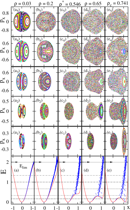
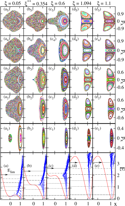
Figure 1: Poincaré sections (upper five rows) depicting the classical dynamics of $\hat{H}^{I}_{\mathrm{int}}(\rho)$ (1) and $\hat{H}^{II}_{\mathrm{int}}(\xi)$ (2) with $h_{2}\!=\!1,\,\beta_{0}\!=\!1.35$, for several values of $\rho\leq\rho_{c}$ and $\xi>\xi_{c}$. The bottom row displays the corresponding classical potentials $V^{(I)}(\rho)$ (3) and $V^{(II)}(\xi)$ (4) and the five energies, below the domain boundary $E_{\mathrm{lim}}\!=\!V(\beta\!=\!\sqrt{2},\gamma)$, at which the sections were calculated. The Peres lattices $\{x_{i},E_{i}\}$, portraying the quantum dynamics for eigenstates with $L\!=\!0$ and $N\!=\!80$, are overlayed on the classical potentials $V(x,y=0)$. They exhibit sequences of regular states in the vicinity of the deformed well, consisting of bandhead states of the ground $g(K=0)$, $\beta^{n}(K=0)$, $\beta^{n}\gamma^{2}(K=0)$, $\beta^{n}\gamma^{4}(K=0)$ bands, etc.

The classical dynamics of $L\!=\!0$ vibrations, governed by $\hat{H}_{\mathrm{int}}$, can be depicted conveniently via Poincaré sections. These are shown in Fig. 1 for selected energies and control parameters. For $\rho\!=\!0$, the system is integrable, with $V^{I}(\rho\!=\!0)\!\propto\!\beta_{0}^{2}\beta^{2}+\textstyle{\frac{1}{2}}(1\!-\!\beta_{0}^{2})\beta^{4}$. The sections for $\rho\!=\!0.03$ in Fig. 1, show the phase space portrait typical of an anharmonic (quartic) oscillator with two major regular islands, weakly perturbed by the small $\rho\cos 3\gamma$ term. For small $\beta$, $V^{I}(\rho)\!\approx\!\beta^{2}\!-\!\rho\sqrt{2}\beta^{3}\cos 3\gamma$. The derived phase-space portrait, shown for $\rho\!=\!0.2$ in Fig. 1, is similar to the Hénon-Heiles system (HH) [10] with regularity at low energy [panels (b₁)-(b₂)] and marked onset of chaos at higher energies [panels (b₃)-(b₅)]. The chaotic component of the dynamics increases with $\rho$ and maximizes at the spinodal point $\rho^{*}\!=\!0.546$. The dynamics changes profoundly in the coexistence region, shown for $\rho\!=\!0.65,\,0.741$ and $\xi\!=\!0.05$ in Fig. 1. As the local deformed minimum develops, robustly regular dynamics attached to it appears. The trajectories form a single island and remain regular at energies well above the barrier height $V_{b}$, clearly separated from the surrounding chaotic environment. As $\xi$ increases, the spherical minimum becomes shallower, the HH-like dynamics diminishes and disappears at the anti-spinodal point $\xi^{**}\!=\!0.354$. Regular motion prevails for $\xi\!>\!\xi^{**}$, where the section landscape changes from a single to several regular islands and the dynamics is sensitive to local degeneracies of normal-modes [4].

The quantum manifestations of the rich classical dynamics can be studied via Peres lattices $\{x_{i},E_{i}\}$ [11]. Here $E_{i}$ are the energies of eigenstates $|i\rangle$ of the Hamiltonian and $x_{i}\!\equiv\!\sqrt{2\langle i|\hat{n}_{d}|i\rangle/N}$. The lattices can distinguish regular from irregular states by means of ordered patterns and disordered meshes of points, respectively. The particular choice of $x_{i}$ can associate the states with a given region in phase space through the classical-quantum correspondence $\beta\!=\!x\!\leftrightarrow\!x_{i}$ [3]. The Peres lattices for $L\!=\!0$ eigenstates of $\hat{H}_{\mathrm{int}}$ with $N\!=\!80$, are shown on the bottom row of Fig. 1, overlayed on the classical potentials $V(x,y=0)$. For $\rho\!=\!0$, the Hamiltonian (1) has U(5) dynamical symmetry with a solvable spectrum $E_{i}\!=\!2\bar{h}_{2}[\beta_{0}^{2}N\!-\!1+(1\!-\!\beta_{0}^{2})n_{d}]n_{d}$. For large $N$, the corresponding Peres lattice coincides with $V^{I}(\rho=0)$, a trend seen in Fig. 1. Whenever a deformed minimum occurs in the potential, the Peres lattices exhibit regular sequences of states, localized in the region of the deformed well and persisting to energies well above the barrier. They are related to the regular islands in the Poincaré sections and are well separated from the remaining states, which form disordered (chaotic) meshes of points at high energy. The regular $L\!=\!0$ states form bandheads of $K\!=\!0$ rotational bands. Additional $K$-bands corresponding to multiple $\beta$ and $\gamma$ vibrations, can also be identified. An example of such regular $K\!=\!0,2$ bands for $\hat{H}_{\mathrm{int}}$ at the critical point, is shown in Fig. 2(a). The states in each band have nearly equal values of $\langle\hat{n}_{d}\rangle$, indicating a common intrinsic structure.

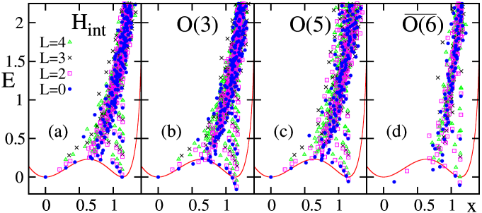
Figure 2: Peres lattices $\{x_{i},E_{i}\}$ for $N\!=\!50,\,L\!=\!0,2,3,4$ eigenstates of $\hat{H}_{\mathrm{int}}^{I}(\rho=\rho_{c})\!=\!\hat{H}_{\mathrm{int}}^{II}(\xi=\xi_{c})$, Eqs. (1)-(2), with $h_{2}\!=\!1,\,\beta_{0}\!=\!1.35$ [panel (a)] and additional collective terms involving $\mathrm{O(3)},\,\mathrm{O(5)}$ and $\overline{\mathrm{O(6)}}$ rotations [panels (b), (c), and (d)]. The classical potential shown, is the same in all cases. Notice in panels (a)-(b)-(c), the well-developed rotational bands ($K\!=\!0$, $L\!=\!0,2,4$) and ($K\!=\!2$, $L\!=\!2,3,4$) formed by the regular states in the deformed phase, which are distorted in panel (d).

The collective part of the Hamiltonian ($\hat{H}_{\mathrm{col}}$), which does not affect $V(\beta,\gamma)$, is composed of the two-body parts of the Casimir operators of the groups $\mathrm{O(3),\,O(5)}$ and $\overline{\mathrm{O(6)}}$ [9]. These orthogonal rotations are associated with the Euler angles, $\gamma$ and $\beta$ degrees of freedom, respectively. Fig. 2 shows the Peres lattices corresponding to $L\!=\!0,2,3,4$ eigenstates of $\hat{H}_{\mathrm{int}}$ at the critical-point, plus added rotational terms one at a time. As seen in Figs. 2(b)-2(c), the $\mathrm{O(3)}$ and $\mathrm{O(5)}$ terms preserve the ordered $K$-bands of $\hat{H}_{\mathrm{int}}$, Fig. 2(a). In contrast, the regular band-structure is strongly disrupted by the $\overline{\mathrm{O(6)}}$ term [Fig. 2(d)]. The latter couples the deformed and spherical configurations [12] and mixes strongly the regular and irregular states. These results demonstrate the advantage of using the resolution $\hat{H}=\hat{H}_{\mathrm{int}}+\hat{H}_{\mathrm{col}}$, since a strong $\overline{\mathrm{O(6)}}$ term in the collective part can obscure the simple patterns of the dynamics disclosed by the intrinsic part.

This work is supported by the Israel Science Foundation. M.M. acknowledges support by the Golda Meir Fellowship Fund and the Czech Ministry of Education (MSM 0021620859).