Electromagnetic helicity wavelets:
a model for quasar engines?

Abstract

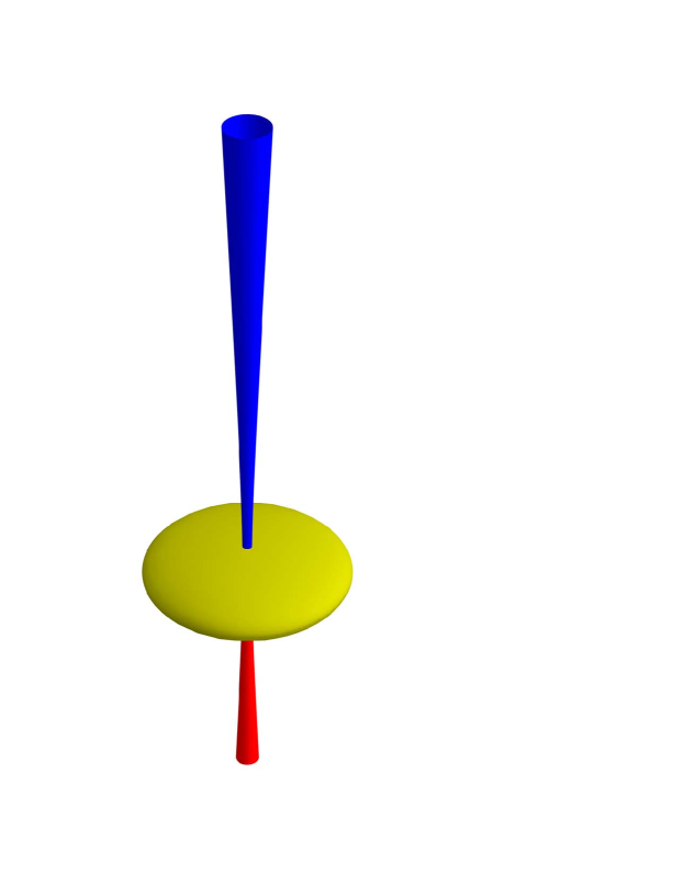
Figure 2: The charge-current densities (40), (42) of the regularized fields $\mbox{\boldmath{{$\tilde{F}$}}}_{\sigma}$ (37) are distributions supported on the union ${\mathcal{\tilde{Q}}}^{\varepsilon,b}$ (36) of a solid oblate spheroid ${\mathcal{\tilde{E}}}^{\varepsilon}$ and two solid semi-hyperboloids ${\mathcal{\tilde{H}}}_{\pm}^{b}$ (35). According to (47), the total electric and magnetic charges vanish, hence ${\mathcal{\tilde{Q}}}^{\varepsilon,b}$ acts as an electric-magnetic dipole antenna. ${\mathcal{H}}^{\varepsilon}_{\pm}$ support the electric dipole and ${\mathcal{\tilde{E}}}^{\varepsilon}$ supports the magnetic dipole, and the flow of electric and magnetic currents within and between ${\mathcal{\tilde{H}}}_{\pm}^{b}$ and ${\mathcal{\tilde{E}}}^{\varepsilon}$ is determined by the analytic signal $g{(\tau)}$ (16). In the ‘bare’ (unregularized) limit ($\varepsilon\to 0,b\to a$), ${\mathcal{\tilde{E}}}^{b}$ approaches the branch disk ${\mathcal{D}}$ and ${\mathcal{\tilde{H}}}_{\pm}^{b}$ approach ${\mathcal{Z}}_{\pm}$, so ${\mathcal{\tilde{Q}}}^{\varepsilon,b}\to{\mathcal{Q}}$ (7). As explained in the text, ${\mathcal{\tilde{Q}}}^{\varepsilon,b}$ could be used to model quasar engines, with ${\mathcal{\tilde{E}}}^{\varepsilon}$ and ${\mathcal{\tilde{H}}}_{\pm}^{b}$ representing the accretion disk and the jets, respectively.

The complex distance function $\zeta$, which plays a prominent role in the definition of scalar (acoustic) wavelets, is found to determine a complex extension of the spherical coordinate system that is ideally suited for the construction of highly focused electromagnetic beams with helicities conforming to the oblate spheroidal geometry of $\zeta$. This is used to build a basis of electromagnetic wavelets ${\boldsymbol{F}}^{m}={\boldsymbol{E}}^{m}+i{\boldsymbol{B}}^{m}$ radiated or absorbed by the branch disk ${\mathcal{D}}$ of $\zeta$. ${\boldsymbol{F}}^{m}$ has integer angular momentum $m$ around the axis of ${\mathcal{D}}$ and definite spheroidal helicity. We use a regularization method to compute its singular charge-current density and show that the total charge vanishes. Hence ${\boldsymbol{F}}^{m}$ is due solely to electric and magnetic polarization currents. ${\mathcal{D}}$ acts as a magnetic dipole antenna, and its axis as a coupled electric dipole antenna. We propose this as an idealized electromagnetic model for quasars (without gravity, i.e., in flat spacetime), with ${\mathcal{D}}$ representing the accretion disk and the vortex singularities along its axis representing the jets. In the regularized version, the accretion disk is represented by a solid, flat oblate spheroid and the jets by two solid, narrow semi-hyperboloids, as shown in Figure 2.

1 The complex helicity basis

A rich geometry ensues when the Euclidean distance in ${{\mathbb{R}}^{n}}$ is continued analytically [K0]. Here we specialize to ${{\mathbb{R}}^{3}}$ and use the notation introduced in [HK9]. Define the complexification $\zeta$ of the radial coordinate $r$ by

$$\zeta=\sqrt{({\boldsymbol{r}}-i{\boldsymbol{a}})^{2}}=\sqrt{\rho^{2}+{\tilde{z}}^{2}}\equiv\xi-i\eta,\ \ {\boldsymbol{r}}=(x,y,z)\in{{\mathbb{R}}^{3}},$$ (1)

$${\boldsymbol{a}}=a\mbox{\boldmath{{$\rm\hat{z}$}}},\quad\rho=\sqrt{x^{2}+y^{2}},\quad{\tilde{z}}=z-ia.$$

The singularity of $r$ at the origin expands to the branch circle of $\zeta$,

$${\mathcal{C}}\equiv\{{\boldsymbol{r}}:\zeta=0\}=\{(x,y,z):x^{2}+y^{2}\equiv a^{2},\ z=0\},$$

and continuation of $\zeta$ along any simple closed loop linking with ${\mathcal{C}}$ gives $-\zeta$. Hence $\zeta$ is double-valued. To make it single-valued, it is necessary to close ${\mathcal{C}}$ with any membrane whose boundary is ${\mathcal{C}}$, the simplest of which is the disk

$${\mathcal{D}}=\{(x,y,z):x^{2}+y^{2}\leq a^{2},\ z=0\}=\{{\boldsymbol{r}}:\xi=0\}.$$

${\mathcal{D}}$ is a branch cut of $\zeta$, and we choose the branch with $\xi\geq 0$ which reduces to $+r$ when $a\to 0$. On crossing ${\mathcal{D}}$, $\eta$ changes sign. As shown in the Appendix (48), $(\xi,\eta)$ are related to the cylindrical coordinates $(\rho,z)$ by

$$az=\xi\eta,\qquad a^{2}\rho^{2}=(a^{2}+\xi^{2})(a^{2}-\eta^{2}),$$

hence $-a\leq\eta\leq a$. Far from ${\mathcal{D}}$, we have

$$r\gg a\ \Rightarrow\ \xi\approx r\ \ \hbox{and}\ \ \eta\approx\mbox{\boldmath{{$\rm\hat{a}$}}}\cdot{\boldsymbol{r}}=a\cos\theta.$$ (2)

The level sets of $\xi$ and $\eta$ define an oblate spheroidal coordinate system, as explained in Figure 1 (see [HK9] for details).

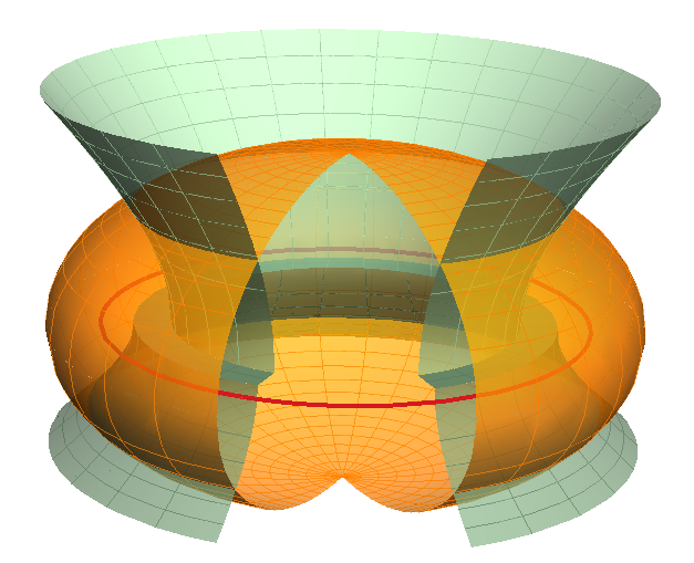
Figure 1: The real and imaginary parts of $\zeta=\xi-i\eta$ form an oblate spheroidal coordinate system with the $z$ axis along ${\boldsymbol{a}}$. Shown are cut-away views of an oblate spheroid ${\mathcal{E}}$ with $\xi=\varepsilon\,(\varepsilon=0.7a)$, a semi-hyperboloid ${\mathcal{H}}_{+}$ with $\eta=b\,(b=0.8a)$, and a semi-hyperboloid ${\mathcal{H}}_{-}$ with $\eta=-b^{\prime}\,(b^{\prime}=0.5a)$. Also shown is the branch circle ${\mathcal{C}}=\partial{\mathcal{D}}$, which is spanned by the branch disk ${\mathcal{D}}$. ${\mathcal{C}}$ is the common focal circle of all the spheroids and hyperboloids. As $\varepsilon\to 0$, ${\mathcal{E}}$ shrinks to a double cover of ${\mathcal{D}}$. As $b\to a$, ${\mathcal{H}}_{\pm}$ shrink to the positive and negative $z$ axis. According to (2), the spheroids ${\mathcal{E}}$ are deformations of the spheres $r=$ constant and the semi-hyperboloids ${\mathcal{H}}_{\pm}$ are deformations of the cones $a\cos\theta=$ constant, whose vertex ${\boldsymbol{r}}={\boldsymbol{0}}$ expands to the circle $\{{\boldsymbol{r}}:\rho=\sqrt{a^{2}-\eta^{2}},\,z=0\}$.

We now use $\zeta$ to defined a complexified version $\vartheta$ of the polar coordinate $\theta$:

$$\sin\vartheta=\frac{\rho}{\zeta},\quad\cos\vartheta=\frac{{\tilde{z}}}{\zeta}.$$ (3)

Like $\zeta$, $\vartheta$ is singular on ${\mathcal{C}}$ and discontinuous on the interior of ${\mathcal{D}}$. By applying the gradient operator with respect to ${\boldsymbol{r}}$ to the coordinates $(\zeta,\vartheta,\phi)$, we obtain vectors $(\mbox{\boldmath{{$\rm\hat{\zeta}$}}},\mbox{\boldmath{{$\rm\hat{\vartheta}$}}},\mbox{\boldmath{{$\rm\hat{\phi}$}}})$ extending the spherical basis $(\mbox{\boldmath{{$\rm\hat{r}$}}},\mbox{\boldmath{{$\rm\hat{\theta}$}}},\mbox{\boldmath{{$\rm\hat{\phi}$}}})$:

$$\rm\hat{\zeta} \equiv\nabla\zeta=\frac{{\boldsymbol{r}}-i{\boldsymbol{a}}}{\zeta}=\frac{\mbox{\boldmath{{$\rm\hat{\rho}$}}}\rho+\mbox{\boldmath{{$\rm\hat{z}$}}}{\tilde{z}}}{\zeta}=\mbox{\boldmath{{$\rm\hat{\rho}$}}}\sin\vartheta+\mbox{\boldmath{{$\rm\hat{z}$}}}\cos\vartheta$$

$$\nabla\vartheta =\frac{\mbox{\boldmath{{$\rm\hat{\vartheta}$}}}}{\zeta}\ \ \hbox{where}\ \ \mbox{\boldmath{{$\rm\hat{\vartheta}$}}}=\mbox{\boldmath{{$\rm\hat{\rho}$}}}\cos\vartheta-\mbox{\boldmath{{$\rm\hat{z}$}}}\sin\vartheta$$

$$\nabla\phi =\frac{\mbox{\boldmath{{$\rm\hat{\phi}$}}}}{\rho}=\frac{\mbox{\boldmath{{$\rm\hat{\phi}$}}}}{\zeta\sin\vartheta}.$$

These vectors form a complex-orthogonal, oriented basis in ${{\mathbb{C}\hskip 0.5pt}^{3}}$, i.e.,

$$\mbox{\boldmath{{$\rm\hat{\zeta}$}}}^{2}=\mbox{\boldmath{{$\rm\hat{\vartheta}$}}}^{2}=\mbox{\boldmath{{$\rm\hat{\phi}$}}}^{2}=1,\quad\mbox{\boldmath{{$\rm\hat{\zeta}$}}}\cdot\mbox{\boldmath{{$\rm\hat{\vartheta}$}}}=\mbox{\boldmath{{$\rm\hat{\vartheta}$}}}\cdot\mbox{\boldmath{{$\rm\hat{\phi}$}}}=\mbox{\boldmath{{$\rm\hat{\phi}$}}}\cdot\mbox{\boldmath{{$\rm\hat{\zeta}$}}}=0$$

$$\mbox{\boldmath{{$\rm\hat{\zeta}$}}}\times\mbox{\boldmath{{$\rm\hat{\vartheta}$}}}=\mbox{\boldmath{{$\rm\hat{\phi}$}}},\quad\mbox{\boldmath{{$\rm\hat{\vartheta}$}}}\times\mbox{\boldmath{{$\rm\hat{\phi}$}}}=\mbox{\boldmath{{$\rm\hat{\zeta}$}}},\quad\mbox{\boldmath{{$\rm\hat{\phi}$}}}\times\mbox{\boldmath{{$\rm\hat{\zeta}$}}}=\mbox{\boldmath{{$\rm\hat{\vartheta}$}}}.$$

In this basis, the gradient operator is

$$\nabla=\mbox{\boldmath{{$\rm\hat{\zeta}$}}}\partial_{\zeta}+\frac{\mbox{\boldmath{{$\rm\hat{\vartheta}$}}}}{\zeta}\partial_{\vartheta}+\frac{\mbox{\boldmath{{$\rm\hat{\phi}$}}}}{\zeta\sin\vartheta}\partial_{\phi}.$$

We now define a related basis which will be especially useful for studying electromagnetic radiation. Let

$$\kappa=\ln\tan(\vartheta/2)=\frac{1}{2}\ln\frac{1-\cos\vartheta}{1+\cos\vartheta}=\frac{1}{2}\ln\frac{\zeta-{\tilde{z}}}{\zeta+{\tilde{z}}},$$

so that

$$\frac{{\rm d}\kappa}{{\rm d}\vartheta}=\frac{1}{\sin\vartheta}.$$ (4)

Let

$$\psi_{\pm}\equiv\phi\pm i\kappa,\qquad\partial_{\pm}\equiv\frac{\partial}{\partial\psi_{\pm}}=\frac{1}{2}\left(\partial_{\phi}\mp i\partial_{\kappa}\right)$$

and define the vectors

$${\boldsymbol{\chi}}_{\pm}\equiv\nabla\psi_{\pm}=\frac{\mbox{\boldmath{{$\rm\hat{\phi}$}}}}{\rho}\pm\frac{i}{\sin\vartheta}\frac{\mbox{\boldmath{{$\rm\hat{\vartheta}$}}}}{\zeta}=\frac{\mbox{\boldmath{{$\rm\hat{\phi}$}}}\pm i\mbox{\boldmath{{$\rm\hat{\vartheta}$}}}}{\rho}.$$ (5)

Note that the factor ${\rm d}\kappa/{\rm d}\vartheta$ transforms the singularity $1/\zeta$ of $\nabla\vartheta$ into the singularity $1/\rho$ of $\nabla\phi$, so that $\rm\hat{\phi}$ and $\rm\hat{\vartheta}$ can be combined into $\mbox{\boldmath{{$\rm\hat{\phi}$}}}\pm i\mbox{\boldmath{{$\rm\hat{\vartheta}$}}}$. This combination will be the key to helicity in our system, and $(\mbox{\boldmath{{$\rm\hat{\zeta}$}}},{\boldsymbol{\chi}}_{+},{\boldsymbol{\chi}}_{-})$ will be called the helicity basis.

Applying the chain rule in the coordinate system $(\zeta,\psi_{+},\psi_{-})$ gives the gradient operator in the helicity basis:

$$\nabla=\mbox{\boldmath{{$\rm\hat{\zeta}$}}}\partial_{\zeta}+{\boldsymbol{\chi}}_{+}\partial_{+}+{\boldsymbol{\chi}}_{-}\partial_{-}\,.$$

Note that

$$\mbox{\boldmath{{$\rm\hat{\zeta}$}}}\cdot{\boldsymbol{\chi}}_{\pm}={\boldsymbol{\chi}}_{\pm}^{2}=0, {\boldsymbol{\chi}}_{+}\cdot{\boldsymbol{\chi}}_{-}=\frac{2}{\rho^{2}}$$ (6)

$$\mbox{\boldmath{{$\rm\hat{\zeta}$}}}\times{\boldsymbol{\chi}}_{\pm}=\pm i{\boldsymbol{\chi}}_{\pm}, {\boldsymbol{\chi}}_{+}\times{\boldsymbol{\chi}}_{-}=\frac{2i\mbox{\boldmath{{$\rm\hat{\zeta}$}}}}{\rho^{2}},$$

so ${\boldsymbol{\chi}}_{\pm}$ are a pair of null, transversal eigenvectors of the operator $\mbox{\boldmath{{$\rm\hat{\zeta}$}}}\times$ with eigenvalues $\pm i$. We shall see that the eigenvalue $i$ corresponds to advanced (absorbed) solutions and $-i$ corresponds to retarded (emitted) solutions.

In addition to the complex angular coordinates $\psi_{\pm}$, define the complex retarded and advanced time coordinates

$$u=\tau-\zeta,\quad v=\tau+\zeta,\ \ \hbox{where}\ \ \tau=t-is$$

is complexified time [K11] and we have chosen units in which the speed of light $c=1$. The functions $(u,v,\psi_{+},\psi_{-})$ form a null coordinate system in spacetime related to the Newman-Penrose formalism.

Note that $(u,v)$ are singular on ${\mathcal{D}}$ and $\psi_{\pm}$ are singular on the $z$ axis (5). Hence our coordinate system is singular on the set

$${\mathcal{Q}}=\{{\boldsymbol{r}}:\xi=0\}\cup\{{\boldsymbol{r}}:\rho=0\}={\mathcal{D}}\cup{\mathcal{Z}}_{+}\cup{\mathcal{Z}}_{-},$$ (7)

where ${\mathcal{Z}}_{+}$ and ${\mathcal{Z}}_{-}$ are the positive and negative $z$ axis, respectively. We shall see that these coordinates are particularly well suited for representing electromagnetic fields radiated or absorbed by ${\mathcal{D}}$. The coordinate singularities will be natural for describing sources on ${\mathcal{Q}}$, just the singularity of the spherical coordinate system $(r,\theta,\phi)$ at the origin is natural for describing point sources at $r=0$.

2 EM fields in the helicity basis

We consider the class of real electromagnetic fields $({\boldsymbol{E}},{\boldsymbol{B}})$ represented in the complex coordinates $(u,v,\psi_{\pm})$ by

$${\boldsymbol{E}}+i{\boldsymbol{B}}\equiv{\boldsymbol{F}}=\alpha{\boldsymbol{C}}+\beta{\boldsymbol{\chi}}_{+}+\gamma{\boldsymbol{\chi}}_{-},$$ (8)

where

$${\boldsymbol{C}}=-\nabla\frac{2}{\zeta}=\frac{2\mbox{\boldmath{{$\rm\hat{\zeta}$}}}}{\zeta^{2}}$$

is the complexified Coulomb field [N73] and $\alpha,\beta,\gamma$ are analytic functions of $(u,v,\psi_{\pm})$ when ${\boldsymbol{r}}\notin{\mathcal{Q}}$. The advantage of the representation (8) is that

$$\nabla\times{\boldsymbol{C}}=\nabla\times{\boldsymbol{\chi}}_{\pm}={\boldsymbol{0}},$$

which will make it easy to compute $\nabla\times{\boldsymbol{F}}$, and

$${\boldsymbol{r}}\notin{\mathcal{Q}}\ \Rightarrow\ \nabla\cdot{\boldsymbol{C}}=\nabla\cdot{\boldsymbol{\chi}}_{\pm}=0,$$ (9)

which will make it easy to compute $\nabla\cdot{\boldsymbol{F}}$ outside of ${\mathcal{Q}}$.

The charge-current density $(\varrho,{\boldsymbol{J}})$ of ${\boldsymbol{F}}$ is defined  [K3] by

$$\varrho\equiv\nabla\cdot{\boldsymbol{F}}\ \ \hbox{and}\ \ -{\boldsymbol{J}}\equiv\partial_{t}{\boldsymbol{F}}+i\nabla\times{\boldsymbol{F}},$$ (10)

where the derivatives must be interpreted in a distributional sense and will be seen to be distributions (generalized functions) supported on ${\mathcal{Q}}$. We shall compute these sources by regularizing the field ${\boldsymbol{F}}$ and then taking the limit as the regularization is removed. But first, let us find the conditions on $(\alpha,\beta,\gamma)$ which make ${\boldsymbol{F}}$ a solution of the homogeneous Maxwell equations outside the singularity set ${\mathcal{Q}}$.

Note that

$$\partial_{t}\alpha=\alpha_{u}+\alpha_{v}\ \ \hbox{and}\ \ \partial_{\zeta}\alpha=\alpha_{v}-\alpha_{u},$$ (11)

where the subscripts denote partial derivatives, and the same goes for $\beta,\gamma$. Taking the divergence of (8) and using the properties of ${\boldsymbol{C}}$ and ${\boldsymbol{\chi}}_{\pm}$ gives

$$\varrho=2\frac{\alpha_{v}-\alpha_{u}}{\zeta^{2}}+2\frac{\beta_{-}+\gamma_{+}}{\rho^{2}}.$$ (12)

Furthermore,

$$\partial_{t}{\boldsymbol{F}} =2\frac{\alpha_{u}+\alpha_{v}}{\zeta^{2}}\mbox{\boldmath{{$\rm\hat{\zeta}$}}}+(\beta_{u}+\beta_{v}){\boldsymbol{\chi}}_{+}+(\gamma_{u}+\gamma_{v}){\boldsymbol{\chi}}_{-}$$

$$i\nabla\alpha\times{\boldsymbol{C}} =i(\alpha_{+}{\boldsymbol{\chi}}_{+}+\alpha_{-}{\boldsymbol{\chi}}_{-})\times\frac{2\mbox{\boldmath{{$\rm\hat{\zeta}$}}}}{\zeta^{2}}=\frac{2\alpha_{+}}{\zeta^{2}}{\boldsymbol{\chi}}_{+}-\frac{2\alpha_{-}}{\zeta^{2}}{\boldsymbol{\chi}}_{-}$$

$$i\nabla\beta\times{\boldsymbol{\chi}}_{+} =i(\beta_{v}-\beta_{u})\mbox{\boldmath{{$\rm\hat{\zeta}$}}}\times{\boldsymbol{\chi}}_{+}+i\beta_{-}{\boldsymbol{\chi}}_{-}\times{\boldsymbol{\chi}}_{+}=(\beta_{u}-\beta_{v}){\boldsymbol{\chi}}_{+}+\frac{2\beta_{-}}{\rho^{2}}\mbox{\boldmath{{$\rm\hat{\zeta}$}}}$$

$$i\nabla\gamma\times{\boldsymbol{\chi}}_{-} =i(\gamma_{v}-\gamma_{u})\mbox{\boldmath{{$\rm\hat{\zeta}$}}}\times{\boldsymbol{\chi}}_{-}+i\gamma_{+}{\boldsymbol{\chi}}_{+}\times{\boldsymbol{\chi}}_{-}=(\gamma_{v}-\gamma_{u}){\boldsymbol{\chi}}_{-}-\frac{2\gamma_{+}}{\rho^{2}}\mbox{\boldmath{{$\rm\hat{\zeta}$}}}.$$

Collecting terms, we have

$$\hskip-12.91663pt-{\boldsymbol{J}} =2\mbox{\boldmath{{$\rm\hat{\zeta}$}}}\left[\frac{\alpha_{u}+\alpha_{v}}{\zeta^{2}}+\frac{\beta_{-}-\gamma_{+}}{\rho^{2}}\right]+2{\boldsymbol{\chi}}_{+}\left[\beta_{u}+\frac{\alpha_{+}}{\zeta^{2}}\right]+2{\boldsymbol{\chi}}_{-}\left[\gamma_{v}-\frac{\alpha_{-}}{\zeta^{2}}\right].$$ (13)

Requiring the sources (12) and (13) to vanish outside the singularity set ${\mathcal{Q}}$, the homogeneous Maxwell equations are thus equivalent to

$$(\alpha_{v}-\alpha_{u})\sin^{2}\vartheta+\beta_{-}+\gamma_{+}=0\,$$

$$(\alpha_{u}+\alpha_{v})\sin^{2}\vartheta+\beta_{-}-\gamma_{+}=0\,$$

$$\alpha_{+}-\zeta^{2}\beta_{u}=0\,$$

$$\alpha_{-}+\zeta^{2}\gamma_{v}=0.$$

By simplifying and using

$$\sin\vartheta=\frac{1}{\cosh\psi},\quad\cos\vartheta=\tanh\psi,\quad\psi=\frac{\psi_{+}+\psi_{-}}{2},\quad\zeta^{2}=\frac{(u-v)^{2}}{4},$$

this can be expressed in terms of of the coordinates $(u,v,\psi_{\pm})$ as

$$\hskip-8.61108pt\boxed{\ \alpha_{u}=\gamma_{+}\cosh^{2}\psi,\ \ \alpha_{v}=-\beta_{-}\cosh^{2}\psi,\ \ \alpha_{+}=\zeta^{2}\beta_{u},\ \ \alpha_{-}=-\zeta^{2}\gamma_{v}.\ }$$ (14)

These equations, which relate the longitudinal component $\alpha$ of the field to its transversal components $\beta,\gamma$, express the homogeneous Maxwell equations in the coordinate system $(u,v,\psi_{\pm})$.

Newman’s holomorphic Coulomb field, representing the electromagnetic part of a spinning, charged (Kerr-Newman) black hole (i.e., ignoring gravity) [N73], is obtained by choosing

$$\alpha=\frac{1}{2},\quad\beta=\gamma=0\ \Rightarrow\ {\boldsymbol{F}}=\frac{\mbox{\boldmath{{$\rm\hat{\zeta}$}}}}{\zeta^{2}}=-\nabla\frac{1}{\zeta}.$$

As proved in [K4], the charge-current density in this case is that of a disk ${\mathcal{D}}$ spinning rigidly at the extreme relativistic angular velocity $\omega=c/a$, so that the boundary ${\mathcal{C}}=\partial{\mathcal{D}}$ spins at the speed of light. This kind of singular behavior is expected of black holes.

The coherent electromagnetic wavelets constructed in [K11],

$${\boldsymbol{F}}=g^{\prime}(\tau-\zeta){\boldsymbol{\chi}}_{-}\,,$$ (15)

are obtained by choosing

$$\alpha=\beta=0,\quad\gamma=g^{\prime}{(u)},$$

which solves (14). Again, these are extreme solutions of Maxwell’s equations whose energy propagates at the speed of light everywhere outside the singularity set ${\mathcal{Q}}$; see [K11b, K12] for a detailed discussion.

The function $g^{\prime}$ in (15) is the complex derivative of the analytic signal $g$ of an arbitrary pulse function $g_{0}{(t)}$, defined by

$$g{(\tau)}=\frac{1}{2\pi i}\int_{-\infty}^{\infty}\frac{g_{0}(t^{\prime})\,{\rm d}t^{\prime}}{\tau-t^{\prime}},\quad\tau=t-is,\quad s\neq 0.$$ (16)

This is a special case of the multidimensional analytic-signal transform [K3, K11a]. If $g_{0}{(t)}$ is at all reasonable (e.g., square-integrable), then $g(t-is)$ is analytic outside the real axis and its real and imaginary parts are smeared version (to scale $|s|$) of $g_{0}{(t)}$ and its Hilbert transform, respectively. The farther we get from the real time axis (by increasing $|s|$), the more smeared out and weaker the analytic signal $g(t-is)$ becomes, and the same goes for its complex derivative $g^{\prime}(t-is)$. Since

$$g^{\prime}(\tau-\zeta)=g^{\prime}(t-\xi-i(s-\eta)),$$

it follows that $g^{\prime}(\tau-\zeta)$ is analytic for $s>a$ (since then $s-\eta\geq s-a>0$ for all ${\boldsymbol{r}}$) and $s<-a$ (since then $s-\eta\leq s+a<0$ for all ${\boldsymbol{r}}$). If $s>a$, $g(\tau-\zeta)$ peaks when $\eta=a$ (the positive $z$ axis ${\mathcal{Z}}_{+}$), and if $s<-a$, it peaks when $\eta=-a$ (the negative $z$ axis ${\mathcal{Z}}_{-}$). Hence $g(\tau-\zeta)$ is a beam-shaping pulse function, forming a beam along ${\mathcal{Z}}_{+}$ or ${\mathcal{Z}}_{-}$ (depending on the choice of $s$) through its dependence on $\zeta$. Such pulses are the basis for complex-source pulsed-beams in the engineering literature; see [HF89] and the detailed references given in [HK9].

3 Electric-magnetic dipoles and quasar engines

Equations (14) also have solutions representing non-axially symmetric generalizations of (15). The simplest ones are

$${\boldsymbol{F}}_{+}=\beta(u,v,\psi_{\pm}){\boldsymbol{\chi}}_{+}\qquad{\boldsymbol{F}}_{-}=\gamma(u,v,\psi_{\pm}){\boldsymbol{\chi}}_{-}$$ (17)

where (14) require that

$$\beta_{u}=\beta_{-}=0\ \ \hbox{and}\ \ \gamma_{v}=\gamma_{+}=0,$$

respectively. Thus ${\boldsymbol{F}}_{+}$ must be advanced (absorbed) and independent of $\psi_{-}$, and ${\boldsymbol{F}}_{-}$ must be retarded (emitted) and independent of $\psi_{+}$:

$${\boldsymbol{F}}_{+}=\beta(\tau+\zeta,\psi_{+}){\boldsymbol{\chi}}_{+}\ \ \hbox{and}\ \ {\boldsymbol{F}}_{-}=\gamma(\tau-\zeta,\psi_{-}){\boldsymbol{\chi}}_{-}$$ (18)

where the dependence on $\phi$ through $\psi_{\pm}$ must be continuous and periodic. It is easy to verify directly that ${\boldsymbol{F}}_{\pm}$ satisfy the homogeneous Maxwell equations outside ${\mathcal{Q}}$, so their charge-current densities must be supported on ${\mathcal{Q}}$.

The fields (18) are null:

$${\boldsymbol{F}}_{\pm}^{2}\equiv({\boldsymbol{E}}_{\pm}+i{\boldsymbol{B}}_{\pm})^{2}=0,\ \ \hbox{{\it i.e., }}\ \ {\boldsymbol{E}}_{\pm}^{2}-{\boldsymbol{B}}_{\pm}^{2}={\boldsymbol{E}}_{\pm}\cdot{\boldsymbol{B}}_{\pm}=0.$$ (19)

These are the conditions of pure radiation everywhere outside ${\mathcal{Q}}$. As proved in [K11, K11b], this means that ${\boldsymbol{F}}_{\pm}$ propagate without leaving any reactive (rest) energy behind; all their energy flows at the speed of light $c$, which is not true of generic EM fields, even in vacuum. Normally, electromagnetic energy flows at speeds $v<c$ in the near zone due, among other things, to interference between field components propagating in different directions.

Thus ${\boldsymbol{F}}_{\pm}$ are extreme. To obtain ‘normal’ solutions whose energies flow at speeds less than $c$ in the near zone, we must include a longitudinal component $\alpha(u,v,\psi_{\pm})\neq 0$. This makes (14) more difficult to solve and will be pursued elsewhere.

By (6), ${\boldsymbol{F}}_{\pm}$ satisfies

$$\mbox{\boldmath{{$\rm\hat{\zeta}$}}}\times{\boldsymbol{F}}_{\pm}=\pm i{\boldsymbol{F}}_{\pm},$$ (20)

and we have seen that ${\boldsymbol{F}}_{\pm}$ depends on time only through $\tau\pm\zeta$. We have interpreted this by saying that ${\boldsymbol{F}}_{+}$ is absorbed and ${\boldsymbol{F}}_{-}$ is emitted. To confirm this, consider the limit of (6) as $a\to 0$, where $\mbox{\boldmath{{$\rm\hat{\zeta}$}}}\to\mbox{\boldmath{{$\rm\hat{r}$}}}$:

$$\mbox{\boldmath{{$\rm\hat{r}$}}}\times{\boldsymbol{F}}_{\pm}=\pm i{\boldsymbol{F}}_{\pm}\ \Leftrightarrow\ \mbox{\boldmath{{$\rm\hat{r}$}}}\times{\boldsymbol{E}}_{\pm}=\mp{\boldsymbol{B}}_{\pm}\ \ \hbox{and}\ \ \mbox{\boldmath{{$\rm\hat{r}$}}}\times{\boldsymbol{B}}_{\pm}=\pm{\boldsymbol{E}}_{\pm}.$$ (21)

This gives the Poynting vectors

$${\boldsymbol{S}}_{\pm}\equiv{\boldsymbol{E}}_{\pm}\times{\boldsymbol{B}}_{\pm}=\mp{\boldsymbol{E}}_{\pm}\times(\mbox{\boldmath{{$\rm\hat{r}$}}}\times{\boldsymbol{E}}_{\pm})=\mp{\boldsymbol{E}}_{\pm}^{2}\,\mbox{\boldmath{{$\rm\hat{r}$}}},$$ (22)

so the energy of ${\boldsymbol{F}}_{+}$ flows inward to the origin and that of ${\boldsymbol{F}}_{-}$ flows outward from the origin. This is indeed consistent with ${\boldsymbol{F}}_{+}$ being absorbed and ${\boldsymbol{F}}_{-}$ being emitted.

Let us derive the spheroidal version of (22). It follows from (20) that the Poynting vector is given by

$$\mp 2{\boldsymbol{S}}_{\pm}=\pm i{\boldsymbol{F}}_{\pm}^{*}\times{\boldsymbol{F}}_{\pm}={\boldsymbol{F}}_{\pm}^{*}\times(\mbox{\boldmath{{$\rm\hat{\zeta}$}}}\times{\boldsymbol{F}}_{\pm})=|{\boldsymbol{F}}_{\pm}|^{2}\mbox{\boldmath{{$\rm\hat{\zeta}$}}}-(\mbox{\boldmath{{$\rm\hat{\zeta}$}}}\cdot{\boldsymbol{F}}_{\pm}^{*}){\boldsymbol{F}}_{\pm},$$

hence

$$\mp{\boldsymbol{S}}_{\pm}=U_{\pm}\mbox{\boldmath{{$\rm\hat{\zeta}$}}}-\frac{1}{2}(\mbox{\boldmath{{$\rm\hat{\zeta}$}}}\cdot{\boldsymbol{F}}_{\pm}^{*}){\boldsymbol{F}}_{\pm}$$ (23)

where

$$U_{\pm}=\frac{1}{2}|{\boldsymbol{F}}_{\pm}|^{2}=\frac{1}{2}({\boldsymbol{E}}_{\pm}^{2}+{\boldsymbol{B}}_{\pm}^{2})={\boldsymbol{E}}_{\pm}^{2}$$

is the energy density. The left side of (23) is real while the right side is complex. Since $\mbox{\boldmath{{$\rm\hat{\zeta}$}}}^{*}\cdot{\boldsymbol{F}}_{\pm}^{*}=0$ and $\mbox{\boldmath{{$\rm\hat{\zeta}$}}}+\mbox{\boldmath{{$\rm\hat{\zeta}$}}}^{*}=2\nabla\xi$, (23) can be rewritten as

$$\mp{\boldsymbol{S}}_{\pm}=U_{\pm}\mbox{\boldmath{{$\rm\hat{\zeta}$}}}-(\nabla\xi\cdot{\boldsymbol{F}}_{\pm}^{*}){\boldsymbol{F}}_{\pm}=U_{\pm}\mbox{\boldmath{{$\rm\hat{\zeta}$}}}-\nabla\xi\cdot({\boldsymbol{E}}_{\pm}-i{\boldsymbol{B}}_{\pm})({\boldsymbol{E}}_{\pm}+i{\boldsymbol{B}}_{\pm}).$$

Taking the real part of both sides gives

$$\mp{\boldsymbol{S}}_{\pm}=U_{\pm}\nabla\xi-\nabla\xi\cdot{\boldsymbol{E}}_{\pm}{\boldsymbol{E}}_{\pm}-\nabla\xi\cdot{\boldsymbol{B}}_{\pm}{\boldsymbol{B}}_{\pm}=-\nabla\xi\cdot{\,\mathbb{T}}_{\pm}$$ (24)

where ${\,\mathbb{T}}_{\pm}$ is the Maxwell stress tensor of ${\boldsymbol{F}}_{\pm}$. This is the spheroidal version of (22), reducing to the latter as $a\to 0$ since $\nabla\xi\to\mbox{\boldmath{{$\rm\hat{r}$}}}$ and $\nabla\xi\cdot{\boldsymbol{E}}_{\pm},\nabla\xi\cdot{\boldsymbol{B}}_{\pm}$ both vanish.

We now introduce the angular functions

$$Z^{m}_{\pm} \equiv e^{-im\psi_{\pm}}=e^{-im\phi}\tan^{\pm m}(\vartheta/2)=e^{-im\phi}\left(\frac{1\mp\cos\vartheta}{1\pm\cos\vartheta}\right)^{m/2}$$ (25)

$$\quad=e^{-im\phi}\left(\frac{\zeta\mp{\tilde{z}}}{\zeta\pm{\tilde{z}}}\right)^{m/2}\ \ \hbox{with}\ \ m\in{\,\mathbb{Z}},$$

where $m$ must be an integer for $Z^{m}_{\pm}$ to be single-valued. If $\pm m>0$, $\tan^{\pm m}(\vartheta/2)$ is a vortex factor suppressing the positive $z$ axis and amplifying the negative $z$ axis; if $\pm m<0$, it does the reverse. This can be seen by noting that $z=\xi\eta/a$ (48), hence

$$\zeta\pm{\tilde{z}}=(\xi-i\eta)\pm(z-ia)=(\xi\pm z)\mp i(a\pm\eta)=\frac{\xi\mp ia}{a}(a\pm\eta)$$

and

$$\zeta\pm{\tilde{z}}=0\ \Leftrightarrow\ \eta=\mp a\ \Leftrightarrow\ \rho=0,\ \mp z\geq 0.$$

Define the basic null helicity wavelets with angular momentum $m$ about the $z$ axis by

$$\boxed{\ {\boldsymbol{F}}^{m}_{\pm}=g^{\prime}(\tau\pm\zeta)Z^{m}_{\pm}{\boldsymbol{\chi}}_{\pm}\,.\ }$$ (26)

They form a Fourier basis for absorbed and emitted helicity fields analytic in $\psi_{\pm}$ and periodic in $\phi$.

To explain and justify the term helicity wavelets, start with the time-harmonic case. From (16) it follows that

$$g_{0}{(t)}=e^{-i\omega t}\ \Rightarrow\ g(t-is)={\,\rm Sgn\,}s\cdot H(\omega s)e^{-i\omega(t-is)},$$ (27)

where $H$ is the Heaviside function (see also [K3, page R298]). Hence

$$g^{\prime}(\tau\pm\zeta)=-i\omega{\,\rm Sgn\,}(s\pm\eta)H(\omega(s\pm\eta))e^{-i\omega(t\pm\xi)}e^{-\omega(s\pm\eta)}.$$

At any fixed position ${\boldsymbol{r}}\notin{\mathcal{Q}}$,

$${\boldsymbol{F}}^{m}_{\pm}=Ae^{-i\omega t}{\boldsymbol{\chi}}_{\pm}=\frac{A}{\rho}\,e^{-i\omega t}(\mbox{\boldmath{{$\rm\hat{\phi}$}}}\pm i\mbox{\boldmath{{$\rm\hat{\vartheta}$}}}),$$ (28)

where $A$ is a complex function of ${\boldsymbol{r}},{\boldsymbol{a}},s,m$ and $\omega$. If $s>0$, then $\omega>0$ by (27) and (28) shows that the polarization of ${\boldsymbol{F}}^{m}_{-}$ spins clockwise about the vector ${\boldsymbol{r}}$, as viewed from the origin, and that of ${\boldsymbol{F}}^{m}_{+}$ spins counterclockwise. Since ${\boldsymbol{F}}_{-}$ is retarded and ${\boldsymbol{F}}_{+}$ is advanced, both wavelets have negative helicity for $\omega>0$; that is, the polarization of ${\boldsymbol{F}}_{+}$ spins clockwise when viewed in the direction of propagation, toward the origin. If $\omega<0$, these spins are reversed. Thus we have shown:

For time-harmonic signals, the wavelets ${\boldsymbol{F}}^{m}_{\pm}$ have helicity  $-{\,\rm Sgn\,}\omega$.

Furthermore, the above concept of helicity makes sense even when $g_{0}$ is not time-harmonic. From (27) it follows that for a general signal, $g{(\tau)}$ consists of the positive-frequency part of $g_{0}$ if $s>0$ and the negative-frequency part of $g_{0}$ if $s<0$:

$$s>0 \ \Rightarrow\ g{(\tau)}=\frac{1}{2\pi}\int_{0}^{\infty}{\rm d}\omega\,e^{-i\omega t-\omega s}{\hat{g}}_{0}{(\omega)}\equiv g_{0}^{+}{(\tau)}$$

$$s<0 \ \Rightarrow\ g{(\tau)}=-\frac{1}{2\pi}\int_{-\infty}^{0}{\rm d}\omega\,e^{-i\omega t-\omega s}{\hat{g}}_{0}{(\omega)}\equiv-g_{0}^{-}{(\tau)},$$

where ${\hat{g}}_{0}{(\omega)}$ is the ordinary Fourier transform of $g_{0}{(t)}$.

• When $s>a$, ${\boldsymbol{F}}_{\pm}$ is a superposition of negative-helicity fields.

• When $s<-a$, ${\boldsymbol{F}}_{\pm}$ is a superposition of positive-helicity fields.

This idea extends to fields of indefinite helicity as follows. Define the helicity operator ${\mathcal{S}}$ on solutions as multiplication by $-{\,\rm Sgn\,}\omega$ in the Fourier domain. This can be expressed directly in the spacetime domain as $-i$ times the temporal Hilbert transform:

$${\mathcal{S}}{\boldsymbol{F}}\equiv\frac{1}{i\pi}\mathchoice{{\vbox{\hbox{$\textstyle-$}}\kern-4.86108pt}}{{\vbox{\hbox{$\scriptstyle-$}}\kern-3.25pt}}{{\vbox{\hbox{$\scriptscriptstyle-$}}\kern-2.29166pt}}{{\vbox{\hbox{$\scriptscriptstyle-$}}\kern-1.875pt}}\!\int_{-\infty}^{\infty}\frac{{\rm d}t^{\prime}}{t^{\prime}-t}{\boldsymbol{F}}({\boldsymbol{r}},t^{\prime})={\boldsymbol{F}}^{-}({\boldsymbol{r}},t)-{\boldsymbol{F}}^{+}({\boldsymbol{r}},t),$$ (29)

where $\mathchoice{{\vbox{\hbox{$\textstyle-$}}\kern-4.86108pt}}{{\vbox{\hbox{$\scriptstyle-$}}\kern-3.25pt}}{{\vbox{\hbox{$\scriptscriptstyle-$}}\kern-2.29166pt}}{{\vbox{\hbox{$\scriptscriptstyle-$}}\kern-1.875pt}}\!\int$ denotes the principal-value integral and ${\boldsymbol{F}}^{\pm}$ denote the positive- and negative frequency parts of ${\boldsymbol{F}}$.

Remark 1. It may be thought unphysical to restrict the time-harmonic field (28) to just positive or just negative frequencies. This would be justified if the opposite component can be obtained by complex conjugation using a reality condition. However, since ${\boldsymbol{F}}$ is complex, its positive- and negative-frequency components are independent. The reality conditions

$${\boldsymbol{E}}_{\omega}{({\boldsymbol{r}})}^{*}={\boldsymbol{E}}_{-\omega}{({\boldsymbol{r}})},\quad{\boldsymbol{B}}_{\omega}{({\boldsymbol{r}})}^{*}={\boldsymbol{B}}_{-\omega}{({\boldsymbol{r}})}$$ (30)

apply only to the Fourier components of the real fields ${\boldsymbol{E}},{\boldsymbol{B}}$. A general time-harmonic field has the complex form

$${\boldsymbol{F}}({\boldsymbol{r}},t)={\boldsymbol{F}}_{\omega}{({\boldsymbol{r}})}e^{-i\omega t}+{\boldsymbol{F}}_{-\omega}{({\boldsymbol{r}})}e^{i\omega t}={\boldsymbol{E}}({\boldsymbol{r}},t)+i{\boldsymbol{B}}({\boldsymbol{r}},t),\quad\omega>0,$$

where ${\boldsymbol{F}}_{\omega}$ and ${\boldsymbol{F}}_{-\omega}$ can be chosen independently. Then the real fields are

$${\boldsymbol{E}} ={\,\rm Re}\ {\boldsymbol{F}}=\frac{1}{2}[{\boldsymbol{F}}_{\omega}+{\boldsymbol{F}}_{-\omega}^{*}]e^{-i\omega t}+\frac{1}{2}[{\boldsymbol{F}}_{-\omega}+{\boldsymbol{F}}_{\omega}^{*}]e^{i\omega t}$$

$${\boldsymbol{B}} ={\,\rm Im}\ {\boldsymbol{F}}=\frac{1}{2i}[{\boldsymbol{F}}_{\omega}-{\boldsymbol{F}}_{-\omega}^{*}]e^{-i\omega t}+\frac{1}{2i}[{\boldsymbol{F}}_{-\omega}-{\boldsymbol{F}}_{\omega}^{*}]e^{i\omega t},$$

so

$${\boldsymbol{E}}_{\omega} =\frac{1}{2}[{\boldsymbol{F}}_{\omega}+{\boldsymbol{F}}_{-\omega}^{*}]={\boldsymbol{E}}_{-\omega}^{*} {\boldsymbol{B}}_{\omega}=\frac{1}{2i}[{\boldsymbol{F}}_{\omega}-{\boldsymbol{F}}_{-\omega}^{*}]={\boldsymbol{B}}_{-\omega}^{*}$$

as required. As we have seen, ${\boldsymbol{F}}_{\omega}{({\boldsymbol{r}})}e^{-i\omega t}$ gives a real field of negative helicity and ${\boldsymbol{F}}_{-\omega}{({\boldsymbol{r}})}e^{i\omega t}$ gives a real field of positive helicity. See [K4a].

Remark 2. Electromagnetic wavelets of definite helicity were already constructed in 1994 [K11a]. However, those wavelets were globally sourceless, hence unrealizable.

4 Regularized charge-current density of ${\boldsymbol{F}}_{\pm}$

Let us write the general helicity fields (18) as

$${\boldsymbol{F}}_{\sigma}({\boldsymbol{r}},t)=g^{\prime}(\tau+{\sigma}\zeta,\psi_{\sigma}){\boldsymbol{\chi}}_{\sigma},\qquad{\sigma}=\pm 1.$$ (31)

They satisfy the homogeneous Maxwell equations everywhere outside the singularity set ${\mathcal{Q}}$:

$${\boldsymbol{r}}\notin{\mathcal{Q}}\ \Rightarrow\ \nabla\cdot{\boldsymbol{F}}=0\ \ \hbox{and}\ \ \partial_{t}{\boldsymbol{F}}_{\sigma}+i\nabla\times{\boldsymbol{F}}_{\sigma}={\boldsymbol{0}},$$ (32)

hence their charge-current density $(\varrho_{\sigma},{\boldsymbol{J}}_{\sigma})$ must be a distribution supported on ${\mathcal{Q}}$. We shall now compute this distribution by regularizing the field ${\boldsymbol{F}}_{\sigma}$ and then applying Maxwell’s equations ‘in reverse’ to compute the sources. Let $\varepsilon>0,\ 0<b<a$, choose differentiable functions $e{(\xi)}$ and $h_{\pm}{(\eta)}$ with

$$e{(\xi)}=\begin{cases}0,&\xi\leq 0\\ 1,&\xi>\varepsilon,\end{cases} h_{\pm}{(\eta)}=\begin{cases}1,&\eta<b\\ 0,&\eta\geq a,\end{cases}$$ (33)

and let

$$R(\xi,\eta)=e{(\xi)}h_{+}{(\eta)}h_{-}(-\eta).$$ (34)

Then

$$R(0,\eta)=R(\xi,\pm a)=0,\ \ \hbox{hence}\ \ {\boldsymbol{r}}\in{\mathcal{Q}}\ \Rightarrow\ R=0.$$

Furthermore, define the solid spheroid ${\mathcal{\tilde{E}}}^{\varepsilon}$ and semi-hyperboloids ${\mathcal{\tilde{H}}}^{b}_{\pm}$

$${\mathcal{\tilde{E}}}^{\varepsilon}=\{{\boldsymbol{r}}:0\leq\xi\leq\varepsilon\}\qquad{\mathcal{\tilde{H}}}^{b}_{\pm}=\{{\boldsymbol{r}}:b\leq\pm\eta\leq a\}$$ (35)

and their union

$${\mathcal{\tilde{Q}}}^{\varepsilon,b}={\mathcal{\tilde{E}}}^{\varepsilon}\cup{\mathcal{\tilde{H}}}^{b}_{+}\cup{\mathcal{\tilde{H}}}^{b}_{-}.$$ (36)

Then

$${\boldsymbol{r}}\notin{\mathcal{\tilde{Q}}}^{\varepsilon,b}\ \Rightarrow\ R=1.$$

As $\varepsilon\to 0$ and $b\to a$, ${\mathcal{\tilde{Q}}}^{\varepsilon,b}\to{\mathcal{Q}}$. We shall regularize ${\boldsymbol{F}}_{\sigma}$ by multiplying it by $R$, thus eliminating the singularity on ${\mathcal{Q}}$ while leaving the field unchanged outside of ${\mathcal{\tilde{Q}}}^{\varepsilon,b}$. We compute the charge-current density of the regularized field and then find the ‘bare’ charge-current density of ${\boldsymbol{F}}_{\sigma}$ as its limit.

Thus define the regularized field

$$\mbox{\boldmath{{$\tilde{F}$}}}_{\sigma}=R{\boldsymbol{F}}_{\sigma}.$$ (37)

Taking the divergence formally, we obtain the charge density of ${\boldsymbol{F}}_{\sigma}$ as

$${\tilde{\varrho}}_{\sigma}\equiv\nabla\cdot\mbox{\boldmath{{$\tilde{F}$}}}_{\sigma} =R\,\nabla\cdot{\boldsymbol{F}}_{\sigma}+\partial_{\xi}R\,\nabla\xi\cdot{\boldsymbol{F}}_{\sigma}+\partial_{\eta}R\,\nabla\eta\cdot{\boldsymbol{F}}_{\sigma}$$

$$=R\,\nabla\cdot{\boldsymbol{F}}_{\sigma}+\frac{{\sigma}a}{\xi^{2}+\eta^{2}}\,g^{\prime}(\tau+{\sigma}\zeta,\psi_{\sigma})(\partial_{\xi}-i\partial_{\eta})R,$$

where we have used (50) and (51) from the Appendix. Assume that as ${\boldsymbol{r}}\to{\mathcal{Q}}$, $R$ vanishes sufficiently rapidly that the first term is identically zero. (This simply requires some smoothness of $R$ at $\xi=0$ and $\eta=\pm a$.) Then

$${\tilde{\varrho}}_{\sigma}=\frac{2{\sigma}a}{\xi^{2}+\eta^{2}}\,g^{\prime}(\tau+{\sigma}\zeta,\psi_{\sigma})\partial_{\zeta}^{*}R\,,$$ (38)

where $\partial_{\zeta}^{*}=\tfrac{1}{2}(\partial_{\xi}-i\partial_{\eta})$ is the partial derivative with respect to the complex conjugate $\zeta^{*}$. In terms of $e$ nd $h_{\pm}$ we have

$${\tilde{\varrho}}_{\sigma}={\tilde{\varrho}}_{\sigma}^{e}+{\tilde{\varrho}}_{\sigma}^{+}+{\tilde{\varrho}}_{\sigma}^{-},$$ (39)

where

$${\tilde{\varrho}}_{\sigma}^{e} =e^{\prime}{(\xi)}h_{+}{(\eta)}h_{-}(-\eta)\nabla\xi\cdot{\boldsymbol{F}}_{\sigma}$$ (40)

$${\tilde{\varrho}}_{\sigma}^{\pm} =\pm e{(\xi)}h^{\prime}_{\pm}(\pm\eta)\nabla\eta\cdot{\boldsymbol{F}}_{\sigma}$$

and we have used the fact that

$$h_{+}^{\prime}(\eta)\neq 0 \ \Rightarrow\ b<\eta<a\ \Rightarrow\ h_{-}(-\eta)=1$$

$$h_{-}^{\prime}(-\eta)\neq 0 \ \Rightarrow\ -a<\eta<-b\ \Rightarrow\ h_{+}(\eta)=1.$$

Similarly, we compute the current density of $\mbox{\boldmath{{$\tilde{F}$}}}_{\sigma}$ as

$$-\mbox{\boldmath{{$\tilde{J}$}}}_{\sigma} \equiv\partial_{t}\mbox{\boldmath{{$\tilde{F}$}}}_{\sigma}+i\nabla\times\mbox{\boldmath{{$\tilde{F}$}}}_{\sigma}$$

$$=R\left(\partial_{t}{\boldsymbol{F}}_{\sigma}+i\nabla\times{\boldsymbol{F}}_{\sigma}\right)+i\partial_{\xi}R\,\nabla\xi\times\mbox{\boldmath{{$\tilde{F}$}}}_{\sigma}+i\partial_{\eta}R\,\nabla\eta\times\mbox{\boldmath{{$\tilde{F}$}}}_{\sigma}.$$

Again, the first term vanishes and we have

$$\mbox{\boldmath{{$\tilde{J}$}}}_{\sigma} =-i\partial_{\xi}R\nabla\xi\times\mbox{\boldmath{{$\tilde{F}$}}}_{\sigma}-i\partial_{\eta}R\nabla\eta\times\mbox{\boldmath{{$\tilde{F}$}}}_{\sigma}$$ (41)

$$=\mbox{\boldmath{{$\tilde{J}$}}}_{\sigma}^{e}+\mbox{\boldmath{{$\tilde{J}$}}}_{\sigma}^{+}+\mbox{\boldmath{{$\tilde{J}$}}}_{\sigma}^{-}$$

where

$$\mbox{\boldmath{{$\tilde{J}$}}}_{\sigma}^{e} =-ie^{\prime}{(\xi)}h_{+}{(\eta)}h_{-}(-\eta)\nabla\xi\times{\boldsymbol{F}}_{\sigma}$$ (42)

$$\mbox{\boldmath{{$\tilde{J}$}}}_{\sigma}^{\pm} =\mp ie{(\xi)}h^{\prime}_{\pm}(\pm\eta)\nabla\eta\times{\boldsymbol{F}}_{\sigma}.$$

Since the supports of $e^{\prime}{(\xi)}$ and $h^{\prime}_{\pm}{(\eta)}$ are $[0,\varepsilon]$ and $[b,a]$, respectively, it follows that $({\tilde{\varrho}}_{\sigma}^{e},\mbox{\boldmath{{$\tilde{J}$}}}_{\sigma}^{e})$ are supported in ${\mathcal{\tilde{E}}}^{\varepsilon}$ and $({\tilde{\varrho}}_{\sigma}^{\pm},\mbox{\boldmath{{$\tilde{J}$}}}_{\sigma}^{\pm})$ are supported in ${\mathcal{\tilde{H}}}^{b}_{\pm}$.

The regularized currents can be expressed compactly by defining

$$\mbox{\boldmath{{$\tilde{v}$}}}_{\sigma}^{e} \equiv-i\frac{\nabla\xi\times{\boldsymbol{\chi}}_{\sigma}}{\nabla\xi\cdot{\boldsymbol{\chi}}_{\sigma}}=-\frac{i{\sigma}\xi}{a}\mbox{\boldmath{{$\rm\hat{z}$}}}+\frac{i{\sigma}\eta}{a}\sqrt{\frac{a^{2}+\xi^{2}}{a^{2}-\eta^{2}}}\,\mbox{\boldmath{{$\rm\hat{\rho}$}}}+\sqrt{\frac{a^{2}+\xi^{2}}{a^{2}-\eta^{2}}}\,\mbox{\boldmath{{$\rm\hat{\phi}$}}}$$ (43)

$$\mbox{\boldmath{{$\tilde{v}$}}}_{\sigma}^{\pm} \equiv-i\frac{\nabla\eta\times{\boldsymbol{\chi}}_{\sigma}}{\nabla\eta\cdot{\boldsymbol{\chi}}_{\sigma}}=-\frac{{\sigma}\eta}{a}\mbox{\boldmath{{$\rm\hat{z}$}}}-\frac{{\sigma}\xi}{a}\sqrt{\frac{a^{2}-\eta^{2}}{a^{2}+\xi^{2}}}\,\mbox{\boldmath{{$\rm\hat{\rho}$}}}+\sqrt{\frac{a^{2}-\eta^{2}}{a^{2}+\xi^{2}}}\,\mbox{\boldmath{{$\rm\hat{\phi}$}}},$$

where we have used the identity $a\rho=\sqrt{m_{\xi}m_{\eta}}$ (48). According to (40) and (42), the currents are given by

$$\mbox{\boldmath{{$\tilde{J}$}}}_{\sigma}^{e}=\mbox{\boldmath{{$\tilde{v}$}}}_{\sigma}^{e}{\tilde{\varrho}}_{\sigma}^{e}\ \ \hbox{and}\ \ \mbox{\boldmath{{$\tilde{J}$}}}_{\sigma}^{\pm}=\mbox{\boldmath{{$\tilde{v}$}}}_{\sigma}^{\pm}{\tilde{\varrho}}_{\sigma}^{\pm}.$$ (44)

Note that

$$\mbox{\boldmath{{$\tilde{v}$}}}_{\sigma}^{e}\cdot\mbox{\boldmath{{$\tilde{v}$}}}_{\sigma}^{e}=1\ \ \hbox{and}\ \ \mbox{\boldmath{{$\tilde{v}$}}}_{\sigma}^{\pm}\cdot\mbox{\boldmath{{$\tilde{v}$}}}_{\sigma}^{\pm}=1,$$ (45)

the significance of which will be investigated elsewhere.

Equations (43) contain a wealth of information. For example, $\mbox{\boldmath{{$\rm\hat{\phi}$}}}\cdot\mbox{\boldmath{{$\tilde{v}$}}}_{\sigma}^{e}$ becomes infinite as ${\boldsymbol{r}}\to{\mathcal{Z}}_{\pm}\,(\eta\to\pm a$), showing that ${\mathcal{\tilde{E}}}^{\varepsilon}$ has vortices there. Since $\mbox{\boldmath{{$\tilde{v}$}}}_{\sigma}^{\pm}$ is real, it relates the electric current density to the electric charge density and the magnetic current density to the magnetic charge density. On the other hand, the $z$ and $\rho$ components of $\mbox{\boldmath{{$\tilde{v}$}}}_{\sigma}^{e}$ are imaginary, so they convert electric to magnetic sources and vice versa.

The unregularized or ‘bare’ sources are obtained by taking the limits $\varepsilon\to 0$ and $b\to a$. By (33),

$$\varepsilon\to 0\ \Rightarrow\ e{(\xi)}\to H{(\xi)}\ \ \hbox{and}\ \ b\to a\ \Rightarrow\ h_{\pm}{(\eta)}\to H(a-\eta),$$

where $H$ is the Heaviside step function. Therefore

$$e^{\prime}{(\xi)}\to\delta{(\xi)},\quad h_{+}^{\prime}{(\eta)}\to-\delta(a-\eta),\quad-h_{-}^{\prime}(-\eta)\to\delta(a+\eta)$$

restrict the sources $(\varrho_{\sigma},{\boldsymbol{J}}_{\sigma})$ to ${\mathcal{D}}$ and ${\mathcal{Z}}_{\pm}$, confirming that the bare sources are indeed distributions supported on these sets. Equations (40) give, after some simplification,

$$\varrho_{\sigma}^{e} =\delta{(\xi)}\frac{{\sigma}a}{\eta^{2}}g^{\prime}(\tau-i{\sigma}\eta,\psi_{\sigma})$$

$$\varrho_{\sigma}^{\pm} =\pm i\delta(a\mp\eta)\frac{{\sigma}a}{\xi^{2}+a^{2}}g^{\prime}(\tau+{\sigma}\xi\mp i\delta a,\psi_{\sigma}),$$

where we have dropped the superfluous factors $H{(\xi)}$ and $H(a\mp\eta)$.

The unregularized versions of $\mbox{\boldmath{{$\tilde{v}$}}}_{\sigma}^{e}$ and $\mbox{\boldmath{{$\tilde{v}$}}}_{\sigma}^{\pm}$ are

$${\boldsymbol{v}}_{\sigma}^{e}=\frac{i{\sigma}\eta\mbox{\boldmath{{$\rm\hat{\rho}$}}}+a\mbox{\boldmath{{$\rm\hat{\phi}$}}}}{\rho}\ \ \hbox{and}\ \ {\boldsymbol{v}}_{\sigma}^{\pm}=\mp{\sigma}\mbox{\boldmath{{$\rm\hat{z}$}}},$$

where we have used the fact that $\sqrt{a^{2}-\eta^{2}}=\rho$ on ${\mathcal{D}}$.

5 The total charge vanishes: no monopoles

As noted above, the regualrized sources ${\tilde{\varrho}}_{\sigma},\mbox{\boldmath{{$\tilde{J}$}}}_{\sigma}$ are complex and their real and imaginary parts are the electric and magnetic charge-current densities for $\mbox{\boldmath{{$\tilde{F}$}}}_{\sigma}$. The total charge ${\tilde{Q}}{(\tau)}$ must be constant due to charge conservation. But if this constant were nonzero, it would have to be real to avoid magnetic monopoles, and this is impossible due to analyticity in $\tau$, unless ${\tilde{Q}}{(\tau)}\equiv 0$. In this section we prove that ${\tilde{Q}}{(\tau)}$ does indeed vanish identically. It suffices to prove this for the regularized basic helicity wavelets

$$\mbox{\boldmath{{$\tilde{F}$}}}_{\sigma}^{m} =R(\xi,\eta){\boldsymbol{F}}_{\sigma}^{m}=R(\xi,\eta)g^{\prime}(\tau+{\sigma}\zeta)e^{-im\psi_{\sigma}}{\boldsymbol{\chi}}_{\sigma}.$$ (46)

The volume element in oblate spheroidal coordinates is given by [K3]

$${\rm d}^{3}{\boldsymbol{r}}=\frac{\xi^{2}+\eta^{2}}{a}\,{\rm d}\xi\,{\rm d}\eta\,{\rm d}\phi,$$

and

$$\int_{0}^{2\pi}{\rm d}\phi\,e^{-im\psi_{\sigma}}=\int_{0}^{2\pi}{\rm d}\phi\,e^{-im\phi\pm m\kappa}=2\pi\delta_{m}^{0}$$

since $\kappa=\ln\tan(\vartheta/2)$ is independent of $\phi$. Equations (38) thus give the total charge of $\mbox{\boldmath{{$\tilde{F}$}}}^{m}_{\sigma}$ as

$${\tilde{Q}}^{m}_{\sigma}{(\tau)} =2\pi{\sigma}\delta_{m}^{0}\int_{0}^{\infty}{\rm d}\xi\int_{-a}^{a}{\rm d}\eta\,g^{\prime}(\tau+{\sigma}\xi-i{\sigma}\eta)\left[\partial_{\xi}R-i\partial_{\eta}R\right].$$

Integrating the first term by parts in $\xi$ and the second term in $\eta$, we obtain

$${\tilde{Q}}^{m}_{\sigma}{(\tau)} =2\pi{\sigma}\delta_{m}^{0}\int_{-a}^{a}{\rm d}\eta\,\left[Rg^{\prime}\right]_{\xi=0}^{\infty}-2\pi i{\sigma}\delta_{m}^{0}\int_{0}^{\infty}{\rm d}\xi\,\left[Rg^{\prime}\right]_{\eta=-a}^{a}$$

$$\quad-4\pi{\sigma}\delta_{m}^{0}\int_{0}^{\infty}{\rm d}\xi\int_{-a}^{a}{\rm d}\eta\,R\,\partial_{\zeta}^{*}g^{\prime}(\tau+{\sigma}\zeta).$$

The first boundary term vanishes because $R(0,\eta)=0$ and

$$\xi\to\infty\ \Rightarrow\ g^{\prime}(\tau+{\sigma}\xi-i{\sigma}\eta)\to 0.$$

The second boundary term vanishes because $R(\xi,\pm a)=0$. Finally, the last term vanishes because $g^{\prime}(\tau+{\sigma}\zeta)$ is analytic in $\zeta=\xi-i\eta$. This proves that

$${\tilde{Q}}^{m}_{\sigma}{(\tau)}\equiv 0$$ (47)

as claimed. Thus $\mbox{\boldmath{{$\tilde{F}$}}}^{m}_{\sigma}$ has neither magnetic nor electric monopoles.

Since the total charge vanishes, the fields $\mbox{\boldmath{{$\tilde{F}$}}}^{m}_{\sigma}$ are due to a combination of electric and magnetic polarizations. Hence the support ${\mathcal{\tilde{Q}}}^{\varepsilon,b}$ (36) of the charge-current density acts as a combined electric-magnetic dipole antenna for receiving $\mbox{\boldmath{{$\tilde{F}$}}}^{m}_{+}$ or emitting $\mbox{\boldmath{{$\tilde{F}$}}}^{m}_{-}$. If ${\mathcal{\tilde{E}}}^{\varepsilon}$ is flat and ${\mathcal{\tilde{H}}}^{b}_{\pm}$ are narrow, meaning that

$$\frac{\varepsilon}{a}\ll 1\ \ \hbox{and}\ \ \frac{a-b}{a}\ll 1,$$

then the electric dipole is supported mostly on ${\mathcal{\tilde{H}}}^{b}_{+}\cup{\mathcal{\tilde{H}}}^{b}_{-}$ and the magnetic dipole is supported mostly on ${\mathcal{\tilde{E}}}^{\varepsilon}$.

We propose this system as an electromagnetic model for quasar engines, with ${\mathcal{\tilde{E}}}^{\varepsilon}$ representing the accretion disk and ${\mathcal{\tilde{H}}}_{\pm}^{b}$ the vortex jets; see Figure 2. It is known that quasars radiate light with a high degree of helicity (circular polarization) [BF2, E3]. Furthermore, since quasars are the most distant visible objects in the universe, they must radiate extremely powerful and highly collimated beams. The radiated wavelets ${\boldsymbol{F}}^{m}_{-}$ in (26) and their regularized versions $\mbox{\boldmath{{$\tilde{F}$}}}^{m}_{-}$ derive their power and collimation from a combination of the beam-shaping properties of $g^{\prime}(\tau-\zeta)$, their angular momentum, and the associated vortex factor $[(\zeta+{\tilde{z}})/(\zeta-{\tilde{z}})]^{m/2}$ in (25).

Remark. The above is a highly idealized and simplified model for quasars. Among other things, it ignores the fact that the accretion disk and the jets of real quasars consist of plasmas and the jets are coupled to the differentially rotating accretion disk by magnetohydrodynamic equations, or preferably a relativistic version thereof. Note that the shape of $e{(\xi)}$ is related to the density of ${\mathcal{\tilde{E}}}^{\varepsilon}$, and the shapes of $h_{\pm}{(\eta)}$ are related to the densities of ${\mathcal{\tilde{H}}}_{\pm}^{b}$. If the plasma dynamics can be expressed in our spheroidal coordinate system, as suggested by Professor Enßlin (private communication), then the coupling between the accretion disk and the jets could perhaps be represented by a relation between $e{(\xi)}$ and $h_{\pm}(\pm\eta)$. This would be an interesting subject for future study.

Appendix

Here we derive various expressions needed for the above computations. From the definition (1) and (3) we have

$$\zeta^{2}=r^{2}-a^{2}-2iaz=(\xi-i\eta)^{2}\ \Rightarrow\ \xi^{2}-\eta^{2}=r^{2}-a^{2},\quad az=\xi\eta$$ (48)

$$a^{2}\rho^{2}=a^{2}r^{2}-a^{2}z^{2}=a^{2}(\xi^{2}-\eta^{2})+a^{4}-\xi^{2}\eta^{2}=m_{\xi}m_{\eta}$$

where

$$m_{\xi}=a^{2}+\xi^{2},\quad m_{\eta}=a^{2}-\eta^{2}.$$

$$\rm\hat{\zeta} =\nabla\xi-i\nabla\eta=\frac{{\boldsymbol{r}}-i{\boldsymbol{a}}}{\zeta}=\frac{\mbox{\boldmath{{$\rm\hat{\rho}$}}}\rho+\mbox{\boldmath{{$\rm\hat{z}$}}}{\tilde{z}}}{\zeta}=\mbox{\boldmath{{$\rm\hat{\rho}$}}}\sin\vartheta+\mbox{\boldmath{{$\rm\hat{z}$}}}\cos\vartheta \mbox{\boldmath{{$\rm\hat{\zeta}$}}}^{2}=1$$

$$\rm\hat{\vartheta} =\mbox{\boldmath{{$\rm\hat{\phi}$}}}\times\mbox{\boldmath{{$\rm\hat{\zeta}$}}}=\mbox{\boldmath{{$\rm\hat{z}$}}}\sin\vartheta-\mbox{\boldmath{{$\rm\hat{\rho}$}}}\cos\vartheta \mbox{\boldmath{{$\rm\hat{\vartheta}$}}}^{2}=1.$$

Taking the real and imaginary parts of $\rm\hat{\zeta}$ and simplifying gives

$$\nabla\xi =\frac{\xi{\boldsymbol{r}}+\eta{\boldsymbol{a}}}{\mu}=\frac{\xi\rho}{\mu}\mbox{\boldmath{{$\rm\hat{\rho}$}}}+\frac{\eta n_{\xi}}{a}\mbox{\boldmath{{$\rm\hat{z}$}}},\ \ \hbox{where}\ \ n_{\xi}=\frac{m_{\xi}}{\mu},\quad\mu=|\xi|^{2}$$

$$\nabla\eta =\frac{\xi{\boldsymbol{a}}-\eta{\boldsymbol{r}}}{\mu}=\frac{\xi n_{\eta}}{a}\mbox{\boldmath{{$\rm\hat{z}$}}}-\frac{\eta\rho}{\mu}\,\mbox{\boldmath{{$\rm\hat{\rho}$}}},\ \ \hbox{where}\ \ n_{\eta}=\frac{m_{\eta}}{\mu}.$$

It follows that

$$|\nabla\xi|^{2}=n_{\xi}\ \ \hbox{and}\ \ |\nabla\eta|^{2}=n_{\eta}.$$

To compute the regularized sources in Section 4, we need expressions for $\nabla\xi\cdot{\boldsymbol{\chi}}_{\sigma},\nabla\eta\cdot{\boldsymbol{\chi}}_{\sigma}$ and $\nabla\xi\times{\boldsymbol{\chi}}_{\sigma},\nabla\eta\times{\boldsymbol{\chi}}_{\sigma}$, where ${\sigma}=\pm$. It follows that

$$\nabla\xi\times\nabla\eta=-\frac{a\rho}{\mu}\mbox{\boldmath{{$\rm\hat{\phi}$}}},$$ (49)

and since $\nabla\xi\cdot\mbox{\boldmath{{$\rm\hat{\phi}$}}}=0$, we have

$$\nabla\xi\cdot{\boldsymbol{\chi}}_{\sigma} =i{\sigma}\nabla\xi\cdot\frac{\mbox{\boldmath{{$\rm\hat{\vartheta}$}}}}{\rho}=i{\sigma}\nabla\xi\cdot\frac{\mbox{\boldmath{{$\rm\hat{\phi}$}}}\times\mbox{\boldmath{{$\rm\hat{\zeta}$}}}}{\rho}=-i{\sigma}\mbox{\boldmath{{$\rm\hat{\phi}$}}}\cdot\frac{\nabla\xi\times\mbox{\boldmath{{$\rm\hat{\zeta}$}}}}{\rho}$$ (50)

$$=-{\sigma}\mbox{\boldmath{{$\rm\hat{\phi}$}}}\cdot\frac{\nabla\xi\times\nabla\eta}{\rho}={\sigma}\frac{a}{\mu}.$$

Furthermore,

$$\mbox{\boldmath{{$\rm\hat{\zeta}$}}}\cdot{\boldsymbol{\chi}}_{\sigma}=(\nabla\xi-i\nabla\eta)\cdot{\boldsymbol{\chi}}_{\sigma}=0\ \Rightarrow\ \nabla\eta\cdot{\boldsymbol{\chi}}_{\sigma}=-i{\sigma}\frac{a}{\mu}.$$ (51)

Equations (50) and (51) will be used in Section 4 to compute the regularized charge densities. To compute the regularized currents, we need the following:

$$\nabla\xi\times\mbox{\boldmath{{$\rm\hat{\phi}$}}} =\frac{\xi\rho}{\mu}\mbox{\boldmath{{$\rm\hat{z}$}}}\,-\frac{\eta n_{\xi}}{a}\mbox{\boldmath{{$\rm\hat{\rho}$}}}\,$$

$$\nabla\xi\times\mbox{\boldmath{{$\rm\hat{\vartheta}$}}} =\nabla\xi\times(\mbox{\boldmath{{$\rm\hat{\phi}$}}}\times\mbox{\boldmath{{$\rm\hat{\zeta}$}}})=|\nabla\xi|^{2}\mbox{\boldmath{{$\rm\hat{\phi}$}}}=n_{\xi}\mbox{\boldmath{{$\rm\hat{\phi}$}}}$$

$$\nabla\eta\times\mbox{\boldmath{{$\rm\hat{\phi}$}}} =-\frac{\eta\rho}{\mu}\mbox{\boldmath{{$\rm\hat{z}$}}}-\frac{\xi n_{\eta}}{a}\mbox{\boldmath{{$\rm\hat{\rho}$}}}$$

$$\nabla\eta\times\mbox{\boldmath{{$\rm\hat{\vartheta}$}}} =\nabla\eta\times(\mbox{\boldmath{{$\rm\hat{\phi}$}}}\times\mbox{\boldmath{{$\rm\hat{\zeta}$}}})=-i|\nabla\eta|^{2}\mbox{\boldmath{{$\rm\hat{\phi}$}}}\,=-in_{\eta}\mbox{\boldmath{{$\rm\hat{\phi}$}}},$$

hence

$$\nabla\xi\times{\boldsymbol{\chi}}_{\sigma} =\frac{\xi}{\mu}\mbox{\boldmath{{$\rm\hat{z}$}}}-\frac{\eta n_{\xi}}{a\rho}\mbox{\boldmath{{$\rm\hat{\rho}$}}}+i{\sigma}\frac{n_{\xi}}{\rho}\mbox{\boldmath{{$\rm\hat{\phi}$}}}$$ (52)

$$\nabla\eta\times{\boldsymbol{\chi}}_{\sigma} =-\frac{\eta}{\mu}\mbox{\boldmath{{$\rm\hat{z}$}}}-\frac{\xi n_{\eta}}{a\rho}\mbox{\boldmath{{$\rm\hat{\rho}$}}}+{\sigma}\frac{n_{\eta}}{\rho}\mbox{\boldmath{{$\rm\hat{\phi}$}}}.$$

References

[1]
[BF2] T Beckert and H Falcke, Circular polarization of radio emission from relativistic jets. A&A 388, 1106–1119, 2002
[E3] T A Enßlin, Is the Long-Term Persistency of Circular Polarization due to the Constant Helicity of the Magnetic Fields in Rotating Quasar Engines? Astrophysics and Space Science Volume 288, Numbers 1-2 (2003), 183–191
[HF89] E Heyman and L B Felsen, Complex source pulsed beam fields,
J. Optical Soc. America 6:806–817, 1989
[K12] G Kaiser, The Reactive Energy of Transient EM Fields. IEEE International Symposium on Antennas and Propagation and USNC-URSI National Radio Science Meeting, Session 563, July 13, 2012
[N73] E T Newman, Maxwell’s equations and complex
Minkowski space, Journal of Mathematical Physics 14:102–103, 1973