Magnetic-field influenced non-equilibrium transport through a quantum ring
with correlated electrons in a photon cavity

Abstract

We investigate magnetic-field influenced time-dependent transport of Coulomb interacting electrons through a two-dimensional quantum ring in an electromagnetic cavity under non-equilibrium conditions described by a time-convolutionless non-Markovian master equation formalism. We take into account the full electromagnetic interaction of electrons and cavity photons without resorting to the rotating wave approximation or reduction to two levels. A bias voltage is applied to semi-infinite leads along the x-axis, which are connected to the quantum ring. The magnetic field is tunable to manipulate the time-dependent electron transport coupled to a photon field with either x- or y-polarization. We find that the lead-system-lead current is strongly suppressed by the y-polarized photon field at magnetic field with two flux quanta due to a degeneracy of the many-body energy spectrum of the mostly occupied states. Furthermore, the current can be significantly enhanced by the y-polarized field at magnetic field with half integer flux quanta.

I introduction

Quantum interference phenomena are essential when developing quantum devices. Quantum confined geometries conceived for such studies may consist of which-path interferometers, Buks et al. (1998); Sprinzak et al. (2000) coupled quantum wires, Bertoni et al. (2000); Gudmundsson and Tang (2006) side-coupled quantum dots, Kobayashi et al. (2004); Valsson et al. (2008) or quantum rings. Szafran and Peeters (2005); Buchholz et al. (2010) These coupled quantum systems have captured interest due to their potential applications in electronic spectroscopy tools Eugster and del Alamo (1991) and quantum information processing. Schroer et al. (2006) Furthermore, the magnetic flux through the ring system can drive persistent currents Cheung et al. (1988) and lead to the topological quantum interference phenomenon known as the Aharonov-Bohm (AB) effect. Aharonov and Bohm (1959); Büttiker et al. (1984); Webb et al. (1985); Tonomura et al. (1986); Pichugin and Sadreev (1997) Both, the persistent current and ring conductance show characteristic oscillations with period of one flux quantum, $\Phi_{0}=hc/e$. Varying either the magnetic field or the electrostatic confining potentials allows the quantum interference to be tuned. Fuhrer et al. (2006)

There has been considerable interest in the study of electronic transport through a quantum system in a strong system-lead coupling regime driven by periodic time-dependent potentials,Tang and Chu (1996); Zeb et al. (2008); Kienle and Léonard (2009); Tang et al. (2011) longitudinally polarized fields,Tang and Chu (1999); Zhou and Li (2005); Jung et al. (2012) or transversely polarized fields.Tang and Chu (2000); Zhou et al. (2003) On the other hand, quantum transport driven by a transient time-dependent potential enables development of switchable quantum devices, in which the interplay of the electronic system with external perturbation plays an important role.Myöhänen et al. (2009); Stefanucci et al. (2010); Tahir and MacKinnon (2010); Chen et al. (2011) These systems are usually operated in the weak system-lead coupling regime and described within the wide-band or the Markovian approximation.Gurvitz and Prager (1996); van Kampen (2001); Harbola et al. (2006) Within this approximation, the energy dependence of the electron tunneling rate or the memory effect in the system are neglected by assuming that the correlation time of the electrons in the leads is much shorter than the typical response time of the central system. However, the transient transport is intrinsically linked to the coherence and relaxation dynamics and cannot generally be described in the Markovian approximation. The energy-dependent spectral density in the leads has to be included for accurate numerical calculation.

In order to explicitly explore the transport dynamics with transient system-lead coupling and electron-photon coupling, a non-Markovian density-matrix formalism involving the energy-dependent coupled elements should be considered based on the generalized master equation (GME).Braggio et al. (2006); Emary et al. (2007); Bednorz and Belzig (2008); Moldoveanu et al. (2009a) How to appropriately describe the carrier dynamics under non-equilibrium conditions with realistic device geometries is a challenging problem.Gudmundsson et al. (2009a, 2010) More recently, manipulation of electron-photon coupled quantum systems embedded in an electromagnetic cavity has become one of the most promising applications in quantum information processing devices. Utilizing the giant dipole moments of inter-subband transitions in quantum wellsHelm (2000); Gabbay et al. (2011) enables researchers to reach the ultrastrong electron-photon coupling regime.Ciuti et al. (2005); Devoret et al. (2007); Abdumalikov et al. (2008) In this regime, the dynamical electron-photon coupling mechanism has to be explored beyond the wide-band and rotating-wave approximations.Zela et al. (1997); Sornborger et al. (2004); Irish (2007) Nevertheless, time-dependent transport of Coulomb interacting electrons through a topologically nontrivial broad ring geometry in an electromagnetic cavity with quantized photon modes remains unexplored beyond the Markovian approximation.

In the present work, we explore the transient effects of electronic transport through a broad quantum ring in a linearly polarized electromagnetic cavity coupled to electrically biased leads. This electron-photon coupled system under investigation can be manipulated by tuning the applied magnetic field and the polarization of the photon field. A time-convolutionless (TCL) version of the GME is utilized to project the time evolution onto the central system by taking trace with respect to the operators in the leads.Davies (1976); Spohn (1980); Breuer et al. (1999) We demonstrate the transient transport properties by showing the many-body (MB) energy spectra, the time-dependence of the electric charge and current, the magnetic-field dependence of the total charge current with (w) or without (w/o) photon cavity, the charge density distribution, the normalized current density distribution and the local current coming from an occupation redistribution of the MB states in the central quantum ring system.

The paper is organized as follows. In Sec. II, the theoretical model is described. The electron system is embedded in an electromagnetic cavity by coupling a many-level electron system with photons using the full photon energy spectrum of a single cavity mode. In Sec. III, we show the numerical results for the dynamical transient transport properties for different magnetic field and photon field polarization. Concluding remarks will be presented in Sec. IV.

II Model and Theory

In this section, we describe the central system potential $V_{S}$ for the broad quantum ring and its connection to the leads. The electronic ring system is embedded in an electromagnetic cavity by coupling a many-level electron system with photons using the full photon energy spectrum of a single cavity mode. The central ring system is described by a MB system Hamiltonian $\hat{H}_{S}$ with a uniform perpendicular magnetic field, in which the electron-electron interaction and the electron-photon coupling to the x- or y-polarized photon field is explicitly taken into account. We employ the TCL-GME approach to explore the non-equilibrium electronic transport when the system is coupled to leads by a transient switching potential.

II.1 Quantum ring connected to leads

The system under investigation is a broad quantum ring connected to left and right leads $l\in\{L,R\}$ with identical parabolic confining potentials

$$V_{l}(\mathbf{r})=\frac{1}{2}m^{*}\Omega_{0}^{2}y^{2},$$ (1)

in which the characteristic energy of the confinement is $\hbar\Omega_{0}=1.0$ meV and $m^{*}=0.067m_{e}$ is the effective mass of an electron in GaAs-based material.

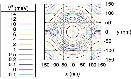
Figure 1: (Color online) Equipotential lines in the central ring system connected to the left and right leads. Note that the isolines are refined close to the bottom of the ring structure.

The quantum ring is embedded in the central system of length $L_{x}=300$ nm situated between two contact areas that will be coupled to the external leads, as is depicted in Fig. 1. The system potential is described by

$$V_{S}(\mathbf{r}) = \sum_{i=1}^{6}V_{i}\exp\left[-\left(\beta_{xi}(x-x_{0})\right)^{2}-\left(\beta_{yi}y\right)^{2}\right]$$ (2)

$$+\frac{1}{2}m^{*}\Omega_{0}^{2}y^{2},$$

with parameters from table 1.

Table 1: Parameters of the central region ring potential.

$i$	$V_{i}$ in meV	$\beta_{xi}$ in $\frac{1}{\mathrm{nm}}$	$x_{0}$ in nm	$\beta_{yi}$ in $\frac{1}{\mathrm{nm}}$
1	9.6	0.014	150	0
2	9.6	0.014	-150	0
3	11.1	0.0165	0	0.0165
4	-4.7	0.02	149	0.02
5	-4.7	0.02	-149	0.02
6	-4.924	0	0	0

II.2 Central system Hamiltonian

The time-evolution of the closed system with respect to $t=0$

$$\hat{U}_{S}(t)=\exp\left(-\frac{i}{\hbar}\hat{H}_{S}t\right)$$ (3)

is governed by the MB system Hamiltonian Gudmundsson et al. (2012)

$$\hat{H}_{S} = \int d^{2}r\;\hat{\psi}^{\dagger}(\mathbf{r})\left[\frac{1}{2m^{*}}\left(\frac{\hbar}{i}\nabla+\frac{e}{c}\left[\mathbf{A}(\mathbf{r})+\hat{\mathbf{A}}^{\mathrm{ph}}(\mathbf{r})\right]\right)^{2}\right.$$ (4)

$$\left.+V_{S}(\mathbf{r})\right]\hat{\psi}(\mathbf{r})+\hat{H}_{ee}+\hbar\omega\hat{a}^{\dagger}\hat{a}\,.$$

The first term includes a constant magnetic field $\mathbf{B}=B\hat{\mbox{\boldmath$z$}}$, in Landau gauge being represented by $\mathbf{A}(\mathbf{r})=-By\hat{\mbox{\boldmath$x$}}$. The second term is the exactly treated electron-electron interaction

$$\hat{H}_{ee}=\int d^{2}r\int d^{2}r^{\prime}\hat{\psi}^{\dagger}(\mathbf{r})\hat{\psi}^{\dagger}(\mathbf{r^{\prime}})V_{ee}(\mathbf{r},\mathbf{r^{\prime}})\hat{\psi}(\mathbf{r^{\prime}})\hat{\psi}(\mathbf{r})\,,$$ (5)

where

$$V_{ee}(\mathbf{r},\mathbf{r^{\prime}})=\frac{e^{2}}{2\kappa\sqrt{|\mathbf{r}-\mathbf{r^{\prime}}|^{2}+\eta^{2}}}$$ (6)

with $e>0$ being the magnitude of the electron charge and $\eta=1.0\times 10^{-15}$ nm being a numerical regularization parameter. In addition, the last term in Eq. (4) indicates the quantized photon field, where $\hat{a}$ and $\hat{a}^{\dagger}$ are the photon annihilation and creation operators, respectively, and $\hbar\omega$ is the photon excitation energy. The photon field interacts with the electron system via the vector potential

$$\hat{\mathbf{A}}^{\mathrm{ph}}(\mathbf{r})=A(\hat{a}+\hat{a}^{\dagger})\begin{cases}\mathbf{e}_{x},&\mathrm{TE}_{011}\\ \mathbf{e}_{y},&\mathrm{TE}_{101}\end{cases}$$ (7)

for longitudinally-polarized (x-polarized) photon field ($\mathrm{TE}_{011}$) or transversely-polarized (y-polarized) photon field ($\mathrm{TE}_{101}$). The electron-photon coupling constant $g^{EM}=eAa_{w}\Omega_{w}/c$ scales with the amplitude $A$ of the electromagnetic field. For reasons of comparison, we also consider results without photons in the system. In this case, $\hat{\mathbf{A}}^{\mathrm{ph}}(\mathbf{r})$ and $\hbar\omega\hat{a}^{\dagger}\hat{a}$ drop out from the MB system Hamiltonian in Eq. (4).

II.3 Time-convolutionless generalized master equation approach

The TCL-GME Breuer et al. (1999) is an alternative non-Markovian master equation to the Nakajima-Zwanzig (NZ) equation,Nakajima (1958); Zwanzig (1960); Gudmundsson et al. (2009b); Moldoveanu et al. (2010) which is local in time. We assume, the initial total statistical density matrix can be written as a product of the system and leads density matrices, before switching on the coupling to the leads,

$$\hat{W}(0)=\hat{\rho}_{L}\otimes\hat{\rho}_{R}\otimes\hat{\rho}_{S}(0),$$ (8)

with $\rho_{l}$, $l\in\{L,R\}$, being the normalized density matrices of the leads. The coupling Hamiltonian between the central system and the leads reads

$$\hat{H}_{T}(t)=\sum_{l=L,R}\int dq\;\chi^{l}(t)\left[\hat{\mathfrak{T}}^{l}(q)\hat{C}_{ql}+\hat{C}_{ql}^{\dagger}\hat{\mathfrak{T}}^{l\dagger}(q)\right]\,.$$ (9)

Here, $\hat{C}_{ql}^{\dagger}$ is the electron creation operator for state $q$ and lead $l$ and

$$\hat{\mathfrak{T}}^{l}(q)=\sum_{\alpha\beta}|\alpha)(\beta|\sum_{a}T_{qa}^{l}(\alpha|\hat{C}_{a}^{\dagger}|\beta)$$ (10)

with the creation operator, $\hat{C}_{a}^{\dagger}$, for the single-electron state (SES) $a$ in the central system, i.e. the eigenstate $a$ of the first term of Eq. (4) with $\hat{\mathbf{A}}^{\mathrm{ph}}(\mathbf{r})=0$. The coupling is switched on at $t=0$ via the switching function

$$\chi^{l}(t)=1-\frac{2}{e^{\alpha^{l}t}+1}$$ (11)

with switching parameter $\alpha^{l}$. Eq. (10) is written in the system Hamiltonian MB eigenbasis $\{|\alpha)\}$. The coupling tensor Gudmundsson et al. (2012)

$$T_{qa}^{l}=\int_{\Omega_{S}^{l}}d^{2}r\;\int_{\Omega_{l}}d^{2}r^{\prime}\;\psi_{ql}^{*}(\mathbf{r^{\prime}})g_{aq}^{l}(\mathbf{r},\mathbf{r^{\prime}})\psi_{a}^{S}(\mathbf{r})$$ (12)

couples the extended lead SES $\{\psi_{ql}(\mathbf{r})\}$ with energy spectrum $\{\epsilon^{l}(q)\}$ to the system SES $\{\psi_{a}^{S}(\mathbf{r})\}$ with energy spectrum $\{E_{a}\}$ that reach into the contact regions, Gudmundsson et al. (2009b) $\Omega_{S}^{l}$ and $\Omega_{l}$, of system and lead $l$, respectively, and

$$g_{aq}^{l}(\mathbf{r},\mathbf{r^{\prime}}) = g_{0}^{l}\exp\left[-\delta_{x}^{l}(x-x^{\prime})^{2}-\delta_{y}^{l}(y-y^{\prime})^{2}\right]$$ (13)

$$\times\exp{\left(-\frac{|E_{a}-\epsilon^{l}(q)|}{\Delta^{l}_{E}}\right)}\,.$$

Here, $g_{0}^{l}$ is the lead coupling strength. In addition, $\delta^{l}_{x}$ and $\delta^{l}_{y}$ are the contact region parameters for lead $l$ in x- and y-direction, respectively. Moreover, $\Delta^{l}_{E}$ denotes the affinity constant between the central system SES energy levels $\{E_{a}\}$ and the lead energy levels $\{\epsilon^{l}(q)\}$.

In this work, we derive the TCL-GME Breuer et al. (1999) in the Schrödinger picture. In this picture, the reduced density operator (RDO) of the system,

$$\hat{\rho}_{S}(t)=\mathrm{Tr}_{L}\mathrm{Tr}_{R}[\hat{W}(t)],$$ (14)

evolves to second order in the lead coupling strength in time via

$$\dot{\hat{\rho}}_{S}(t) = -\frac{i}{\hbar}[\hat{H}_{S},\hat{\rho}_{S}(t)]-\Bigg{[}\sum_{l=L,R}\int dq\;\Big{[}\hat{\mathfrak{T}}^{l}(q),\hat{\Omega}^{l}(q,t)\hat{\rho}_{S}(t)$$ (15)

$$-f(\epsilon^{l}(q))\left\{\hat{\rho}_{S}(t),\hat{\Omega}^{l}(q,t)\right\}\Big{]}+\mathrm{H.c.}\Bigg{]}$$

with

$$\hat{\Omega}^{l}(q,t) = \frac{1}{\hbar^{2}}\chi^{l}(t)\exp\left(-\frac{i}{\hbar}t\epsilon^{l}(q)\right)$$ (16)

$$\times\hat{U}_{S}(t)\hat{\Pi}^{l}(q,t)\hat{U}_{S}^{\dagger}(t),$$

$$\hat{\Pi}^{l}(q,t) = \int_{0}^{t}dt^{\prime}\;\left[\exp\left(\frac{i}{\hbar}t^{\prime}\epsilon^{l}(q)\right)\chi^{l}(t^{\prime})\right.$$ (17)

$$\times\left.\hat{U}_{S}^{\dagger}(t^{\prime})\hat{\mathfrak{T}}^{l\dagger}(q)\hat{U}_{S}(t^{\prime})\right]$$

and $f(E)$ being the Fermi distribution function.

Comparing this equation to the corresponding NZ equation, Nakajima (1958); Zwanzig (1960); Gudmundsson et al. (2009b); Moldoveanu et al. (2010)

$$\dot{\hat{\rho}}_{S}^{\rm NZ}(t) = -\frac{i}{\hbar}[\hat{H}_{S},\hat{\rho}_{S}^{\rm NZ}(t)]$$ (18)

$$-\Bigg{[}\sum_{l=L,R}\int dq\;[\hat{\mathfrak{T}}^{l}(q),\hat{\Omega}^{l}(q,t)]+\mathrm{H.c.}\Bigg{]}$$

with

$$\hat{\Omega}^{l}(q,t) = \frac{1}{\hbar^{2}}\chi^{l}(t)\hat{U}_{S}(t)\int_{0}^{t}dt^{\prime}\;\left[\exp\left(\frac{i}{\hbar}(t^{\prime}-t)\epsilon^{l}(q)\right)\right.$$ (19)

$$\times\left.\chi^{l}(t^{\prime})\hat{\Pi}^{l}(q,t^{\prime})\right]\hat{U}_{S}^{\dagger}(t)$$

and

$$\hat{\Pi}^{l}(q,t^{\prime}) = \hat{U}_{S}^{\dagger}(t^{\prime})\Big{[}\hat{\mathfrak{T}}^{l\dagger}(q)\hat{\rho}_{S}^{\rm NZ}(t^{\prime})$$ (20)

$$-f(\epsilon^{l}(q))\left\{\hat{\rho}_{S}^{\rm NZ}(t^{\prime}),\hat{\mathfrak{T}}^{l\dagger}(q)\right\}\Big{]}\hat{U}_{S}(t^{\prime}),$$

we note that we reobtain the TCL equation, if we set

$$\hat{\rho}_{S}^{\rm NZ}(t^{\prime})=\hat{U}_{S}^{\dagger}(t-t^{\prime})\hat{\rho}_{S}(t)\hat{U}_{S}(t-t^{\prime}),$$ (21)

in Eq. (20) (which enters the kernel of Eq. (18)), but let $\hat{\rho}_{S}^{\rm NZ}(t)=\hat{\rho}_{S}(t)$ in the first term of Eq. (18). In other words, in the Schrödinger picture, the NZ kernel takes the central system time propagated RDO (which lets it become convoluted), while the TCL kernel takes just the unpropagated RDO. The deviation between the two approaches is therefore only of relevance when the central system is far from a steady state and when the coupling to the leads is strong. It is our experience that the positivity conditions Whitney (2008) for the MB state occupation probabilities in the RDO are satisfied to a higher system-lead coupling strength in the TCL case. The more involved quantum structure demands a stronger system-lead coupling than in our earlier work. Gudmundsson et al. (2012) The numerical effort of the two approaches is of similar magnitude. Both cases allow for a $t$-independent inner time integral over $t^{\prime}$, which can be integrated successively with increasing $t$ (increasing integration domain). Moldoveanu et al. (2009b) The RDO is inside (NZ) or outside (TCL) of the inner time integral, but the required number of matrix multiplications is equal.

III Non-equilibrium transport properties

In this section, we investigate the non-equilibrium electron transport properties through a quantum ring system, which is situated in a photon cavity and weakly coupled to leads. We assume GaAs-based material with electron effective mass $m^{*}=0.067m_{e}$ and background relative dielectric constant $\kappa=12.4$. We consider a single cavity mode with fixed photon excitation energy $\hbar\omega=0.4$ meV. The electron-photon coupling constant in the central system is $g^{EM}=0.1$ meV. Before switching on the coupling, we assume the central system to be in the pure initial state with electron occupation number $N_{e,\rm{init}}=0$ and photon occupation number $N_{ph,\rm{init}}=1$ of the electromagnetic field.

An external perpendicular uniform magnetic field is applied through the central ring system and the lead reservoirs. The area of the central ring system is $A\approx 2\times 10^{4}$ $\mathrm{nm}^{2}$ so that the magnetic field corresponding to the flux quantum $\Phi_{0}$ is $B_{0}=\Phi_{0}/A\approx 0.2$ T. The temperature of the reservoirs is assumed to be T = 0.5 K. The chemical potentials in the leads are $\mu_{L}=2$ meV and $\mu_{R}=0.9$ meV leading to a source-drain bias window $\Delta\mu=1.1$ meV. To facilitate inelastic scattering processes between the SES in the central ring system and the SES in the lead $l$, we allow for coupling of highly energetically different states by letting the affinity constant $\Delta_{E}^{l}=4.0$ meV.Abdullah et al. (2010) In addition, we let the contact region parameters for lead $l\in\{L,R\}$ in x- and y-direction be $\delta^{l}_{x}=\delta^{l}_{y}=4.39\times 10^{-4}$ $\rm{nm}^{-2}$. The system-lead coupling strength $g_{0}^{l}=0.2058$ ${\rm meV}/{\rm nm}^{3/2}$.

There are several relevant length and time scales that should be mentioned. The two-dimensional magnetic length is $l=[c\hbar/(eB)]^{1/2}=25.67[B({\rm T})]^{-1/2}$ nm. The ring system is parabolically confined in the y-direction with characteristic energy $\hbar\Omega_{0}=1.0$ meV leading to a modified magnetic length scale

$$a_{w} =\left(\frac{\hbar}{m^{*}\Omega_{0}}\right)^{1/2}\frac{1}{\sqrt[4]{1+[eB/(m^{*}c\Omega_{0})]^{2}}}$$

$$=\frac{33.74}{\sqrt[4]{1+2.982[B({\rm T})]^{2}}}\ {\rm nm}.$$ (22)

Correspondingly, the system-lead coupling strength is then $g_{0}^{l}a_{w}^{3/2}=39.85$ meV for magnetic field $B=0.1$ T and $g_{0}^{l}a_{w}^{3/2}=38.22$ meV for magnetic field $B=0.225$ T. The time-scale for the switching on of the system-lead coupling is $(\alpha^{l})^{-1}=3.291$ ps, the single-electron state (1ES) charging time-scale $\tau_{\rm 1ES}\approx 30$ ps, and the two-electron state (2ES) charging time-scale $\tau_{\rm 2ES}\gg 200$ ps described in the sequential tunneling regime. We study the transport properties for $0\leq t<\tau_{\rm 2ES}$, when the system has not yet reached a steady state.

In order to understand the non-equilibrium dynamical behavior of the charge distribution in the system, we define the time-dependent magnitude of charge on the left part ($x<0$) of the ring

$$Q_{S}^{L}(t)=\int_{-\frac{L_{x}}{2}}^{0}dx\;\int_{-\infty}^{\infty}dy\;\rho(\mathbf{r},t)$$ (23)

and the time-dependent magnitude of charge on the right part ($x>0$) of the ring

$$Q_{S}^{R}(t)=\int_{0}^{\frac{L_{x}}{2}}dx\;\int_{-\infty}^{\infty}dy\;\rho(\mathbf{r},t)\,.$$ (24)

The space- and time-dependent charge density,

$$\rho(\mathbf{r},t)=\mathrm{Tr}[\hat{\rho}_{S}(t)\hat{\rho}(\mathbf{r})],$$ (25)

is the expectation value of the charge density operator

$$\hat{\rho}(\mathbf{r})=e\hat{\psi}^{\dagger}(\mathbf{r})\hat{\psi}(\mathbf{r}).$$ (26)

In order to explore the magnetic field influence on the charge currents from and into the leads, we define the charge current from the left lead into the system by

$$I_{L}(t)=\mathrm{Tr}[\dot{\hat{\rho}}_{S}^{L}(t)\hat{Q}]\,.$$ (27)

Here, $\hat{Q}=e\hat{N}$ is the charge operator with number operator $\hat{N}$ and the time-derivative of the RDO in the MB basis due to the coupling to the lead $l\in\{L,R\}$

$$\dot{\rho}_{S}^{l}(t) = \int dq\;\Big{[}\mathfrak{T}^{l}(q),\Big{[}\Omega^{l}(q,t)\rho_{S}(t)-$$ (28)

$$f(\epsilon^{l}(q))\left\{\rho_{S}(t),\Omega^{l}(q,t)\right\}\Big{]}\Big{]}+\mathrm{H.c.}.$$

Similarly, the charge current from the system into the right lead can be expressed as

$$I_{R}(t)=-\mathrm{Tr}[\dot{\hat{\rho}}_{S}^{R}(t)\hat{N}].$$ (29)

To get more insight into the local current flow in the ring system, we define the top local charge current through the upper arm ($y>0$) of the ring

$$I_{\mathrm{top}}(t)=\int_{0}^{\infty}dy\;j_{x}(x=0,y,t)$$ (30)

and the bottom local charge current through the lower arm ($y<0$) of the ring

$$I_{\mathrm{bottom}}(t)=\int_{-\infty}^{0}dy\;j_{x}(x=0,y,t)\,.$$ (31)

Here, the charge current density,

$$\mathbf{j}(\mathbf{r},t)=\begin{pmatrix}j_{x}(\mathbf{r},t)\\ j_{y}(\mathbf{r},t)\end{pmatrix}=\mathrm{Tr}[\hat{\rho}_{S}(t)\hat{\mathbf{j}}(\mathbf{r})],$$ (32)

is given by the expectation value of the charge current density operator,

$$\hat{\mathbf{j}}(\mathbf{r})=\hat{\mathbf{j}}_{p}(\mathbf{r})+\hat{\mathbf{j}}_{d}(\mathbf{r}),$$ (33)

decomposed into the paramagnetic charge current density operator,

$$\hat{\mathbf{j}}_{p}(\mathbf{r})=\frac{e\hbar}{2mi}\left[\hat{\psi}^{\dagger}(\mathbf{r})(\nabla\hat{\psi}(\mathbf{r}))-(\nabla\hat{\psi}^{\dagger}(\mathbf{r}))\hat{\psi}(\mathbf{r})\right],$$ (34)

and the diamagnetic charge current density operator,

$$\hat{\mathbf{j}}_{d}(\mathbf{r})=\hat{\mathbf{j}}_{d}^{\rm mag}(\mathbf{r})+\hat{\mathbf{j}}_{d}^{\rm ph}(\mathbf{r}).$$ (35)

The latter consists of a magnetic component,

$$\hat{\mathbf{j}}_{d}^{\rm mag}(\mathbf{r})=\frac{e^{2}}{m}\mathbf{A}(\mathbf{r})\hat{\psi}^{\dagger}(\mathbf{r})\hat{\psi}(\mathbf{r}),$$ (36)

and photonic component,

$$\hat{\mathbf{j}}_{d}^{\rm ph}(\mathbf{r})=\frac{e^{2}}{m}\hat{\mathbf{A}}^{\mathrm{ph}}(\mathbf{r})\hat{\psi}^{\dagger}(\mathbf{r})\hat{\psi}(\mathbf{r}).$$ (37)

Furthermore, to understand better the driving schemes of the dynamical transport features, we define the total local charge current

$$I_{\rm tl}(t)=I_{\rm top}(t)+I_{\rm bottom}(t)$$ (38)

and circular local charge current

$$I_{\rm cl}(t)=\frac{1}{2}(I_{\rm top}(t)-I_{\rm bottom}(t)).$$ (39)

Below, we shall explore the influence of the applied magnetic field and the photon fiel polarization on the non-equilibrium quantum transport in terms of the above time-dependent charges and currents in the broad quantum ring system connected to leads.

III.1 Photons with x-polarization

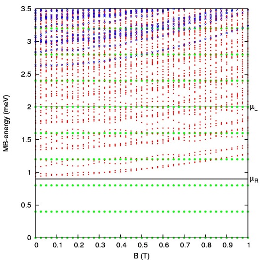
Figure 2: (Color online) MB energy spectrum of system Hamiltonian $\hat{H}_{S}$ versus magnetic field $B$ in units of tesla (T). The states are differentiated according to their electron content $N_{e}$: zero-electron states ($N_{e}=0$, 0ES, green dots), single electron states ($N_{e}=1$, 1ES, red dots) and two electron states ($N_{e}=2$, 2ES, blue crosses). The photon field is x-polarized.

In this subsection, we focus on our results for x-polarized photon field. Figure 2 shows the MB energy spectrum of the system Hamiltonian $\hat{H}_{S}$ including the electron-electron and electron-photon interactions. The MB-energy levels are assigned different colors according to their electron content $N_{e}$. For $N_{e}=0$ (green dots), the MB states differ in energy by multiples of the photon energy $\hbar\omega$ according to their photon content $N_{ph}$ independently of the applied magnetic field. The bias window contains a number of SES (red dots) of which the two lowest ones have the highest occupation. The SESs show crossing behavior at half integer flux quanta. The state-dependent effective magnetic flux ring area allows for small variations of the crossing period $B_{0}$. The crossings at integer flux quanta are usually avoided due to the ring rotation symmetry violation, which is mainly coming from the presence of the central system contact regions to the leads. In general, the SES and, in particular, the two electron states (2ES, blue crosses) tend to increase in energy with higher magnetic field.

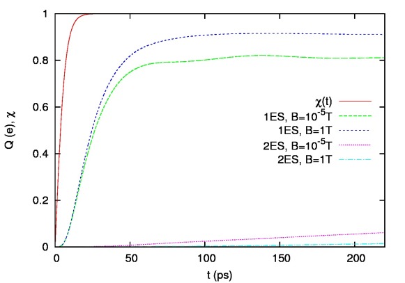
Figure 3: (Color online) Switching function $\chi^{l}(t)$ (solid red), charge of all 1ES for $B=10^{-5}$ T (dashed green) and $B=1.0$ T (dotted blue), and charge of all 2ES for $B=10^{-5}$ T (dotted purple) and $B=1.0$ T (dash-dotted cyan) as a function of time. The photon field is x-polarized.

Figure 3 illustrates the central region charging of 1ES and 2ES as a function of time with the initial conditions $Q_{\rm 1ES}(0)=Q_{\rm 2ES}(0)=0$ since we selected an initial state with $N_{e,\rm{init}}=0$. In the low magnetic field regime, in the case $B=10^{-5}$ T, we notice that $(t,Q_{\rm 1ES})=(200\,{\rm ps},0.809e)$ and $(t,Q_{\rm 2ES})=(200\,{\rm ps},0.055e)$. In the high magnetic field regime, in the case $B=1$ T, we notice that $(t,Q_{\rm 1ES})=(200\,{\rm ps},0.911e)$ and $(t,Q_{\rm 2ES})=(200\,{\rm ps},0.012e)$. In general, the 2ES are occupied slower than the 1ES indicating the sequential tunneling processes. But more importantly, the energetic location of the 2ES and their shifting above the bias window by the Coulomb interaction attenuates the 2ES occupation. As is shown in Fig. 2, the magnetic field plays a role to increase further the energy difference of the 2ES with respect to the 1ES, thus enhancing the 1ES occupation by $\delta Q_{\rm 1ES}=0.102e$ while reducing the 2ES occupation by $\delta Q_{\rm 2ES}=-0.043e$. We note that the earlier mentioned time-scales $(\alpha^{l})^{-1}=3.291$ ps, $\tau_{\rm 1ES}\approx 30$ ps and $\tau_{\rm 2ES}\gg 200$ ps are in agreement with Fig. 3.

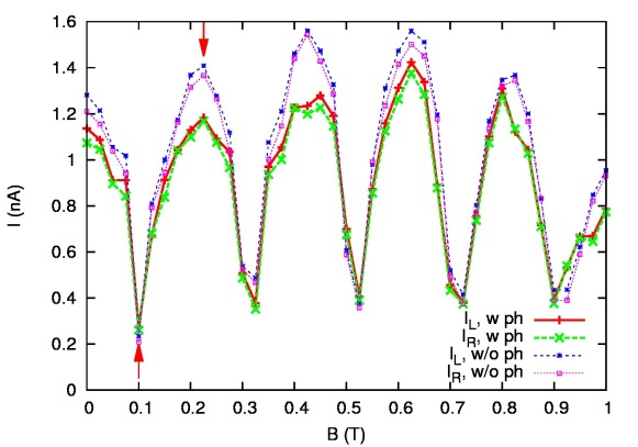
Figure 4: (Color online) The left charge current $I_{L}$ (solid red) and the right charge current $I_{R}$ (long-dashed green) versus the magnetic field with (w) x-polarized photon field at $t=200\mathrm{ps}$. For comparison: left charge current $I_{L}$ (short-dashed blue) and right charge current $I_{R}$ (dotted purple) in a purely electronic central system, i.e. without (w/o) photon cavity.

In Fig. 4, we show the current from the left lead into the ring system $I_{L}$ (solid red curve) and the current from the ring system to the right lead $I_{R}$ (long-dashed green curve) as a function of magnetic field at time $t=200$ ps. The similar values of $I_{L}(B)$ and $I_{R}(B)$ indicate that the short-time regime charging of 1ES is nearly completed at $t=200$ ps meaning that the total charging has slowed down by more than an order of magnitude. Moreover, we see clear oscillations of the current with period $B_{0}\approx 0.2$ T: the first minimum current at $B=0.1$ T corresponds to the situation of a half flux quantum, in which the left charge current $I_{L}=0.273$ nA and the right charge current $I_{R}=0.261$ nA and the maximum current at $B=0.225$ T is corresponding to the case of one flux quantum, in which the left charge current $I_{L}=1.183$ nA and the right charge current $I_{R}=1.168$ nA. These observations are in agreement with the Aharonov-Bohm (AB) oscillations of the steady state Aharonov and Bohm (1959); Büttiker et al. (1984); Webb et al. (1985) but superimposed and modified by electron-electron correlation effects and the non-equilibrium situation. In addition, the electron-photon coupling suppresses the constructive interference of AB-phases in the integer flux quantum situation as can be seen from a comparison with the purely electronic system results in Fig. 4 (short-dashed blue and dotted purple curve).

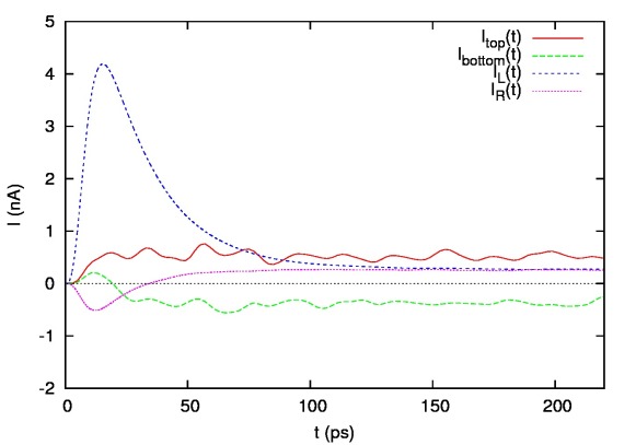
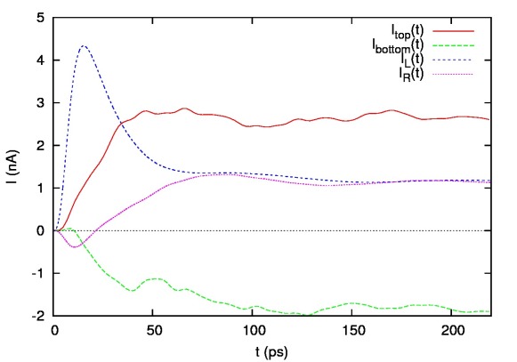
Figure 5: (Color online) Local current through the top ring branch $I_{\mathrm{top}}(t)$, local current through the bottom ring branch $I_{\mathrm{bottom}}(t)$, current from the left lead into the system $I_{L}(t)$, and current from the system into the right lead $I_{R}(t)$ as a function of time for 5 $B=0.1$ T and 5 $B=0.225$ T in the case of x-polarized photon field.

Figure 5 shows the time-evolution of the left total current $I_{L}(t)$, the right total current $I_{R}(t)$, the top local current $I_{\mathrm{top}}(t)$, and the bottom local current $I_{\mathrm{bottom}}(t)$. In the case of $B=0.1$ T (a half flux quantum) shown in Fig. 5(a), the maximum value of the charge current from the left lead at $t=15.30$ ps is $I_{L}=4.190$ nA. In addition, the minimum value of the charge current to the right lead at $t=12.25$ ps is $I_{R}=-0.511$ nA. The negative right charge current indicates that the central system is also charged from the right lead during the transient phase. In the case of $B=0.225$ T (one flux quantum) shown in Fig. 5(b), the maximum value of the current from the left lead at $t=15.35$ ps is $I_{L}=4.334$ nA; and the minimum right charge current at $t=10.80$ ps is $I_{R}=-0.387$ nA. It is then interesting to realize that the magnetic field enhances the charge accumulation from the left lead, while it suppresses the short-time regime charging from the right lead. Hence, the integer magnetic flux quantum case assists the net current flow already in the highly non-equilibrium situation in the very beginning. The local charge transport may differ in direction in the ring arms due to the persistent magnetic field induced ring current.

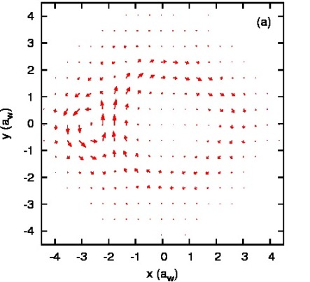
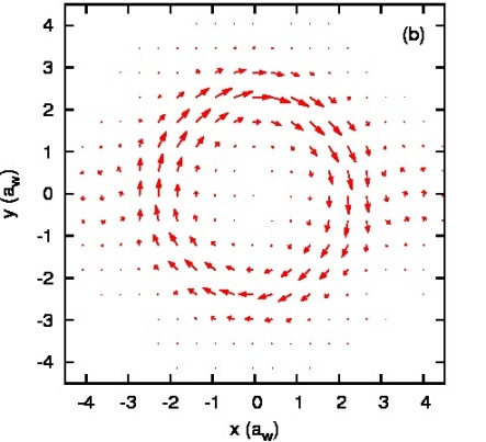
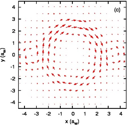
Figure 6: (Color online) Normalized charge current density vector field in the central system for (a) $B=0.1$ T, (b) $B=0.225$ T, and (c) $B=0.425$ T at $t=200$ ps in the case of x-polarized photon field.

In Fig. 6, we illustrate the normalized charge current density vector field $\mathbf{j}(\mathbf{r},t)$ in the central quantum ring system in the case of x-polarized photon field in the long-time response regime $t=200$ ps, i.e. when the 2ES get charged. For magnetic field $B=0.1$ T, a clear counter-clockwise vortex located close to the left lead can be found dominating the current flow pattern in the central ring system as shown in Fig. 6(a). Pichugin and Sadreev (1997) The vortex circulation direction is in agreement with the Lorentz force, since the enclosed area is threaded by much less than half a flux quantum. Due to the geometrical position of the vortex and the current continuity condition, clockwise current direction is favored for the ring system. However, the counter-clockwise vortex appears relatively weak for magnetic field $B=0.225$ T present at both left and right lead connection area as shown in Fig. 6(b), while the total local current through the whole central system from the left to the right lead is large. Additionally, for a later comparison with the y-polarized photon field, Fig. 6(c) shows the current density for $B=0.425$ T (two flux quanta), which is similar to Fig. 6(b) (one flux quanta) with the vortex circulation on both sides being slightly more significant.

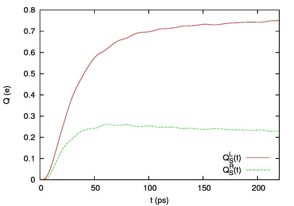
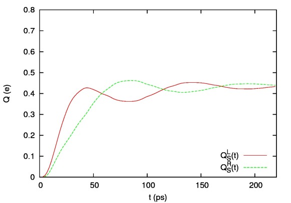
Figure 7: (Color online) Charge in the left ($Q_{S}^{L}(t)$) or right half ($Q_{S}^{R}(t)$) of the central quantum ring system as a function of time for 7 $B=0.1$ T and 7 $B=0.225$ T. The photon field is x-polarized.

Figure 7 illustrates the time-dependent charge on the left part of the ring $Q_{S}^{L}(t)$ and the time-dependent charge on the right part of the ring $Q_{S}^{R}(t)$. In the case of $B=0.1$ T shown in Fig. 7(a), both $Q_{S}^{L}$ and $Q_{S}^{R}$ are increasing almost monotonically in time. In the long-time response regime $t=200$ ps, $Q_{S}^{L}(t)=0.742e$ is much higher than $Q_{S}^{R}(t)=0.234e$. This implies charge accumulation mainly on the left hand side of the quantum ring in the case of magnetic field with half integer flux quantum with enhancement of the electron dwell time on the left-hand side of the ring and suppression of the electron dwell time on the right-hand side.

In the case $B=0.225$ T shown in Fig. 7(b), both $Q_{S}^{L}$ and $Q_{S}^{R}$ exhibit oscillations in time after the short-time charging regime. This implies that the charge accumulation manifests itself in oscillating behavior between the left and the right part of the quantum ring in the case of magnetic field with integer flux quantum. The oscillation amplitude is decreasing in time due to the dissipation effects caused by the coupling to the leads. In the long-time response regime $t=200$ ps, $Q_{S}^{L}(t)=0.423e$ is of similar magnitude than $Q_{S}^{R}(t)=0.446e$, which is by difference to the half integer flux quantum case. It is interesting to notice that the oscillating period of the charges is around $\tau=100$ ps corresponding to a characteristic energy $\delta E_{Q}\approx 0.04$ meV. The MB energies of the mostly occupied MB levels are $E_{10}^{x}=1.4038$ meV $E_{9}^{x}=1.3664$ meV such that $\Delta E_{9,10}^{x}=0.0374$ meV. The corresponding two-level (TL) oscillation period of the closed system would be $\tau_{\rm TL}^{0}=111$ ps. In the non-equilibrium open system, the TL oscillation period is $\tau_{\rm TL}^{L}=94$ ps or $\tau_{\rm TL}^{R}=100$ ps when we take the time intervals between the first and second maxima of $Q_{S}^{L}(t)$ and $Q_{S}^{R}(t)$, respectively. The full numerical calculation including all MB levels shown in Fig. 7(b) yields the left and right charge oscillation period, $\tau^{L}=96$ ps and $\tau^{R}=110$ ps, respectively. The system is far from equilibrium at the earlier maximum, thus reducing in particular the left period $\tau_{\rm TL}^{L}$ with respect to $\tau_{\rm TL}^{0}$. However, we find that also the other MB states change the periods when comparing $\tau^{L}$ with $\tau_{\rm TL}^{L}$ and $\tau^{R}$ with $\tau_{\rm TL}^{R}$.

We would like to bring attention to the fact that charge balances like $\dot{Q}_{L}=I_{L}-I_{\rm tl}$ and $\dot{Q}_{R}=I_{\rm tl}-I_{R}$ would not be satisfied. This is because the SES that are filled from the left lead or emptied to the right lead are in general not restricted to a single half of the central system, but extended over the whole system.

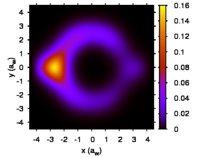
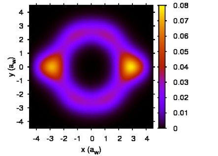
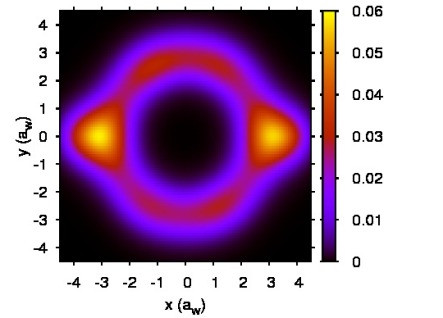
Figure 8: (Color online) Charge density distribution $\rho(\mathbf{r},t)\;(e/a_{w}^{2})$ in the central system for 8 $B=0.1$ T, 8 $B=0.225$ T, and 8 $B=0.425$ T in the x-polarized photon field case at $t=200$ ps.

Figure 8 shows the charge density distribution in the central quantum ring system in the case of x-polarized photon field with the magnetic field 8 $B=0.1$ T, 8 $B=0.225$ T, and 8 $B=0.425$ T at $t=200$ ps. In the case of $B=0.1$ T (half flux quantum) shown in Fig. 78, the electrons are highly accumulated on the left-hand side of the quantum ring with very weak coupling to the right lead, and hence strongly blocking the left charge current and suppressing the right charge current, as it was shown previously in Fig. 4 (marked by the up-arrow). For half integer flux quantum, the electron dwell time on the left-hand side of the ring is enhanced relative to the electron dwell time on the right-hand side of the ring due to destructive phase interference on the right hand side. The density accumulates then mainly on the left hand side of the ring forming a long-living state and the magnetic field evoked vortex on the right hand side contact area is suppressed.

In the $B=0.225$ T case (one flux quantum) shown in Fig. 88, the electrons manifest oscillating feature between the left and right end of the quantum ring. At time $t=200$ ps, the electrons are nearly equally well accumulated on both sides of the quantum ring. This phenomenon is related to the manifestation of current peaks observed in Fig. 4 (marked by the down-arrow). The charge distribution is rearranged when compared to magnetic field $B=0.1$ T. We observe a depletion of about $50\%$ at the left-hand contact region with equivalent charge augmentation on the right-hand contact region. The magnetic field $B=0.225$ T with integer flux quantum enhances the likelihood for electrons to flow through the quantum ring to the right-hand side of the central system and further to the right lead. Additionally, Fig. 88 shows the charge density for $B=0.425$ T (two flux quanta), which is similar to Fig. 88 (one flux quantum).

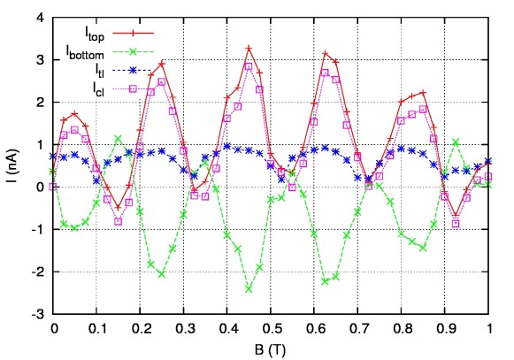
Figure 9: (Color online) Local current through the top arm of the ring $I_{\mathrm{top}}$ (solid red), local current through the bottom arm of the ring $I_{\mathrm{bottom}}$, total local current $I_{\rm tl}$, and the circular local current $I_{\rm cl}$) versus the magnetic field averaged over the time interval $[180,220]\mathrm{ps}$ in the case of x-polarized photon field.

In Fig. 9, we show the magnetic field dependence of the partial local currents $I_{\mathrm{top}}$ and $I_{\mathrm{bottom}}$ through the top and bottom arms, the total local current $I_{\rm tl}$ across $x=0$, and the circular local current $I_{\rm cl}$, which are convenient tools to study the relative importance of local “persistent” current flows induced by the magnetic field in the long-time response transient time regime. We averaged the local currents over the time interval $[180,220]\mathrm{ps}$ around $t=200$ ps to soften possible high frequency fluctuations (compare with Fig. 5). In general, the top local current exhibits opposite sign to the bottom local current, and hence the circular local current (solid purple) is usually larger in magnitude than the total local current (dotted blue). The local current through the two current arms, $I_{\rm tl}$, is strongly suppressed in the case of half integer flux quanta showing a very similar behavior to the nonlocal currents $I_{L}$ and $I_{R}$ (Fig. 4). This is because the destructive interference in the quantum ring enhances the back scattering for magnetic flux with half integer quanta.

In the absence of magnetic field $B=0$, the circular current is identical to zero due to the symmetric situation for both ring arms. Moreover, it is interesting to note that the circular local current $I_{\rm cl}$ reaches $1.347$ nA for less than half a flux quantum (at $B=0.05$ T), increases further until $B=0.45$ T with a maximum value $\max|I_{\rm cl}|=2.844$ nA and decreases again for $B>0.45$ T. The magnetic component of the diamagnetic part of the circular local current increases linearly with the magnetic field $B$, but the paramagnetic part guarantees a behavior, which is closer to being periodic with the flux quantum. The periodic part is in analogy to the behavior for a ring of infinitesimal width. Byers and Yang (1961) In the case of high magnetic field regime ($B>0.45$ T), a comparison with Fig. 2 shows that the different flux periods of different MB-states in the finite-width ring lead to destructive interference effects reducing the periodic oscillations considerably. The most common direction of the circular current is clockwise. This is because the vortices at the lead connection areas are threaded by less than half a flux quantum leading to counter-clockwise vortex rotation direction. Then, as a consequence of charge continuity and the vortex location outside the ring radius, clockwise direction for $I_{\rm cl}$ is preferred.

III.2 Photons with y-polarization

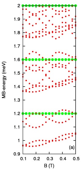
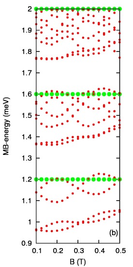
Figure 10: (Color online) MB energy spectrum of the system Hamiltonian $\hat{H}_{S}$ versus magnetic field $B$ within the bias window energy range for (a) x-polarized and (b) y-polarized photon field. The states are differentiated according to their electron content $N_{e}$: zero-electron states ($N_{e}=0$, 0ES, green dots) and single electron states ($N_{e}=1$, 1ES, red dots).

In this subsection, we focus on the y-polarized photon field situation and compare with the results for the x-polarized photon field. Figure 10 shows the MB energy spectra of the system Hamiltonian $\hat{H}_{S}$ in the case of (a) x-polarized and (b) y-polarized photon field. We note in passing that Fig. 10(a) magnifies a part of the MB spectrum of Fig. 2. The mostly occupied levels are the two levels around $1.4$ meV. In the cases of both x- and y-polarized photon field, we see the MB energy degeneracy around $B=0.1$ and $0.325$ T related to the destructive AB phase interference. However, in the case of y-polarization, an extra MB energy degeneracy is found at $B=0.425$ T. This degeneracy is related to a photon suppressed current dip, i.e. not related to AB oscillations.

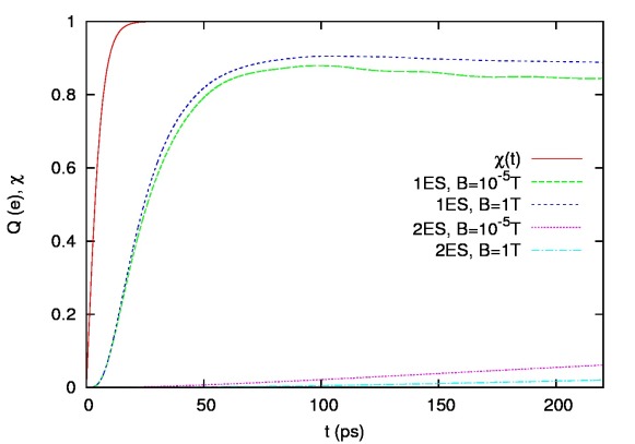
Figure 11: (Color online) Switching function $\chi^{l}(t)$ (solid red), charge of all 1ES for $B=10^{-5}$ T (dashed green) and $B=1.0$ T (dotted blue), and charge of all 2ES for $B=10^{-5}$ T (dotted purple) and $B=1.0$ T (dash-dotted cyan) as a function of time. The photon field is y-polarized.

Figure 11 illustrates the charge of 1ES and 2ES as a function of time. In the case of low magnetic field regime $B=10^{-5}$ T, we notice that $(t,Q_{\rm 1ES})=(200\,{\rm ps},0.847e)$ and $(t,Q_{\rm 2ES})=(200\,{\rm ps},0.055e)$. In the case of high magnetic field regime $B=1$ T, we notice that $(t,Q_{\rm 1ES})=(200\,{\rm ps},0.891e)$ and $(t,Q_{\rm 2ES})=(200\,{\rm ps},0.017e)$. The 2ES are occupied much slower than the 1ES due to similar reasons than for the x-polarized photon field. The magnetic field enhances the 1ES occupation by $\delta Q_{\rm 1ES}=0.044e$ while it suppress the 2ES occupation by $\delta Q_{\rm 2ES}=-0.038e$. Therefore, in comparison with the case of x-polarization shown in Fig. 3, we realize that the y-polarized photon field mildens the influence of the applied magnetic field on the charging feature.

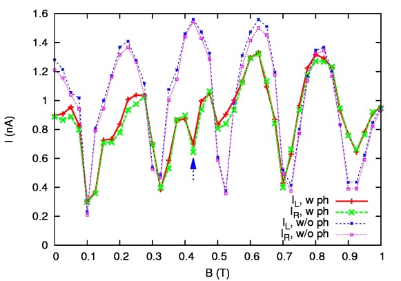
Figure 12: (Color online) Left charge current $I_{L}$ (solid red) and right charge current $I_{R}$ (long-dashed green) versus the magnetic field with (w) y-polarized photon field at $t=200\mathrm{ps}$. For comparison: left charge current $I_{L}$ (short-dashed blue) and right charge current $I_{R}$ (dotted purple) in a purely electronic central system, i.e. without (w/o) photon cavity.

Figure 12 shows the left charge current $I_{L}$ (solid red) and the right charge current $I_{R}$ (dashed green) as a function of magnetic field in the case of y-polarized photon field at $t=200\mathrm{ps}$. The similar values of $I_{L}(B)$ and $I_{R}(B)$ agree well with the long-time response regime slow-down in charging predicted in Fig. 11, which is almost completed for the 1ES. Charge current oscillations are shifted slightly from the period $B_{0}\approx 0.2$ T due to the broad ring geometry. Moreover, the oscillation amplitude and extrema positions show more unexpected features than in the case of x-polarized photon field. The first current minimum is at magnetic field $B=0.1$ T (with a half flux quantum) with left charge current $I_{L}=0.303$ nA and right charge current $I_{R}=0.298$ nA. At magnetic field $B=0.225$ T corresponding to the case of one flux quantum, the left charge current $I_{L}=1.007$ nA and the right charge current $I_{R}=0.935$ nA. It is interesting to point out that the magnetic field dependence of the charge current exhibits a pronounced dip at magnetic field $B=0.425$ T (two flux quanta) in the case of y-polarized photon field that is not present in the case of x-polarized photon field.

The dip structure in the charge current at $B=0.425$ T is due to the above mentioned degeneracy of the MB energy spectrum, which strongly suppresses the photon-assisted tunneling feature. Furthermore, the charge current can be enhanced by the y-polarized photon field at magnetic field with half integer flux quantum: the y-polarized photon field significantly influences the quantum interference of the circular local current flow including the destructive interference feature of the charge current.

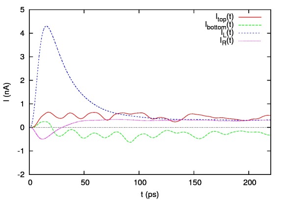
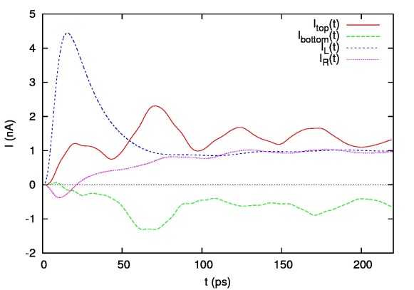
Figure 13: (Color online) Local current through the top ring branch ($I_{\mathrm{top}}(t)$) and bottom ring branch ($I_{\mathrm{bottom}}(t)$), current from the left lead ($I_{L}(t)$) and into the right lead ($I_{R}(t)$) for 13 $B=0.1$ T and 13 $B=0.225$ T in the case of y-polarized photon field.

Figure 13 illustrates the time-evolution of the left total current $I_{L}(t)$, the right total current $I_{R}(t)$, the top local current $I_{\mathrm{top}}(t)$, and the bottom local current $I_{\mathrm{bottom}}(t)$. In the case of $B=0.1$ T shown in Fig. 13(a), the maximum value of the current from the left lead into the system at $t=15.55$ ps is $I_{L}(t)=4.303$ nA. Furthermore, the minimum value of the charge current into the right lead at $t=12.00$ ps is $I_{R}=-0.494$ nA. The negative right charge current indicates that the central system is charged from the left and the right lead for a short time. This charging from the right is a little weaker than in the case of x-polarized photon field. In the case of $B=0.225$ T shown in Fig. 5(b), the maximum value of the left current at $t=15.54$ ps is $I_{L}=4.446$ nA and the minimum value of the right current at $t=10.80$ ps is $I_{R}=-0.337$ nA. Hence, the integer magnetic flux enhances the charge accumulation from the left lead, while it suppresses the short-time regime charging from the right lead assisting the net current flow from the left to the right already in the highly non-equilibrium situation in the very beginning. The local charge transport may differ in direction in the ring arms due to the “persistent” current induced by the magnetic field.

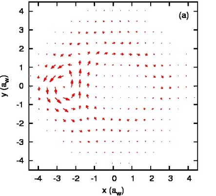
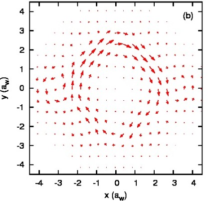
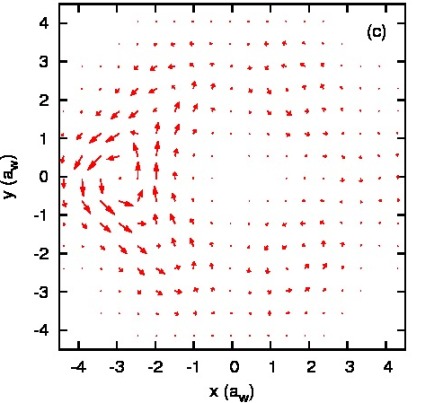
Figure 14: (Color online) Normalized charge current density vector field in the central system for (a) $B=0.1$ T, (b) $B=0.225$ T and (c) $B=0.425$ T at $t=200$ ps in the case of y-polarized photon field.

In Fig. 14, we demonstrate the normalized charge current density vector field $\mathbf{j}(\mathbf{r},t)$ in the central ring system for the magnetic field, (a) $B=0.1$ T, (b) $B=0.225$ T, and (c) $B=0.425$ T, in the long-time response regime $t=200$ ps in the case of y-polarized photon field. For magnetic field $B=0.1$ T, a clear counter-clockwise vortex can be found being associated with a long-living localized state which is strongly dominating the current flow pattern in the central ring system, as is shown in Fig. 14(a). However, for magnetic field $B=0.225$ T, this counter-clockwise vortex appears weaker relative to the total local current, but is present at both contact regions as shown in Fig. 14(b). Figures 14(a) and 14(b) are similar to Figs. 6(a) and 6(b) meaning that the local current flow is mainly governed by AB interference with the photon polarization having only a minor effect.

Figure 14(c) shows the current density for $B=0.425$ T (two flux quanta), which is similar to Fig. 14(a) (a half flux quantum) and not to the one flux quantum case as for x-polarization (similarity between Fig. 6(c) and Fig. 6(b)). This feature is not predicted by the AB effect, but is caused by the influence of the y-polarized photons. However, the impact of a MB spectrum degeneracy of the mostly occupied MB states (Fig. 10(b)) on the local current flow structure is similar whether the degeneracy is in agreement with the AB effect (Fig. 14(a)) or not, i.e. originates from the photons (Fig. 14(c)).

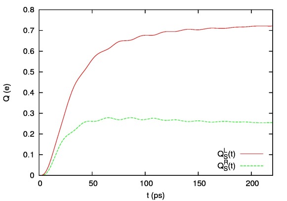
Figure 15: (Color online) Charge in the left half ($Q_{S}^{L}(t)$) or right half ($Q_{S}^{R}(t)$) of the central system as a function of time for 15 $B=0.1$ T and 15 $B=0.225$ T. The photon field is y-polarized.

Figure 15 shows the time-evolution of $Q_{S}^{L}(t)$ and $Q_{S}^{R}(t)$. In the short-time response regime at $t=65$ ps, the charge on the left and right part of the ring are $Q_{S}^{L}=0.548e$ and $Q_{S}^{R}=0.318e$ for $B=0.225$ T, respectively; the charge on the left and right part of the ring are $Q_{S}^{L}=0.610e$ and $Q_{S}^{R}=0.279e$ for $B=0.1$ T. Consequently, the electron dwell time on the left-hand side of the ring is enhanced while the electron dwell time on the right-hand side is suppressed for y-polarized photon field and integer flux quantum; this feature is though more pronounced for a half flux quantum and y-polarized photon field, but was already described for x-polarized photons (Fig. 7(a)). The reason for the difference in left and right dwell time in the integer flux quantum case is a low frequency oscillation of the most important close-in-energy levels. In the long-time response regime at time $t=200$ ps, the picture is very similar to the x-polarized photon field case: for $B=0.225$ T, the left and right charges are of similar magnitude, $Q_{S}^{L}=0.462e$ and $Q_{S}^{R}=0.431e$; and for $B=0.1$ T, the charge is mainly accumulated at the left hand side, $Q_{S}^{L}=0.720e$ and $Q_{S}^{R}=0.256e$.

In the $B=0.225$ T case, the MB energies of the mostly occupied MB levels are $E_{10}^{y}=1.3846$ meV and $E_{9}^{y}=1.3683$ meV such that $\Delta E_{9,10}^{y}=0.0163$ meV. The energy level difference of the mostly occupied MB levels is only $44\%$ of the case of x-polarized photon field: $E_{9,10}^{y}\approx 0.44\times E_{9,10}^{x}$. The corresponding TL oscillation period of the closed system would be $\tau_{\rm TL}^{0}=254$ ps. The oscillation period is too long to be observed clearly in Fig. 1515, but the first maximum of $Q_{S}^{L}(t)$ at $t=65$ ps represents the starting point of the low frequency oscillation, which is better visible in the TL system defined by the two mostly occupied states. Our findings suggest that the energy difference of the two mostly occupied levels controls not only the charge distribution, but also photonic suppressions of the AB current. The different connectivity (probability density on the left or right ring part) to the leads found within the TL dynamic suggests that the probability of a photon coupled electron transition between these levels plays a major role in understanding the photonic modifications of the AB current pattern.

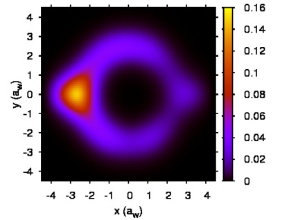
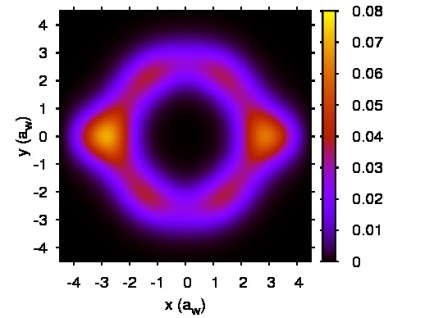
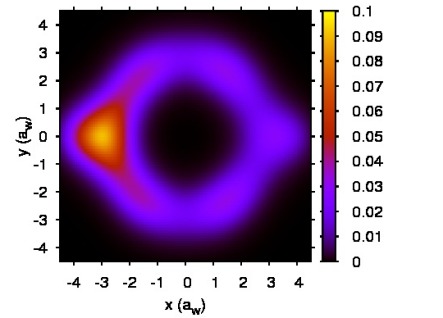
Figure 16: (Color online) Charge density distribution $\rho(\mathbf{r},t)\;(e/a_{w}^{2})$ in the central system for 16 $B=0.1$ T, 16 $B=0.225$ T, and 16 $B=0.425$ T in the y-polarized photon field case at $t=200$ ps.

Figure 16 shows the charge density distribution in the central ring system in the case of y-polarized photon field for magnetic field 16 $B=0.1$ T, 16 $B=0.225$ T, and 16 $B=0.425$ T at $t=200$ ps. In the case of $B=0.1$ T shown in Fig. 1616, the electrons are highly accumulated on the left-hand side of the quantum ring with very weak coupling to the right lead, and hence strongly blocking the left charge current and suppressing the right charge current.

In the case of $B=0.225$ T shown in Fig. 1616, the electrons manifest oscillating feature between the left and right end of the quantum ring. At time $t=200$ ps, the electrons are equally well accumulated on both sides of the quantum ring. This situation is related to the manifestation of the current peaks observed in Fig. 12. The charge is redistributed when compared to magnetic field $B=0.1$ T. We observe a depletion of about $50\%$ on the left-hand side with equivalent charge augmentation on the right hand side. The magnetic field $B=0.225$ T with integer flux quanta enhances the likelihood for electrons to flow through the quantum ring to the right-hand side of the central system and further to the right lead.

Figure 1616 shows the charge density for $B=0.425$ T (two flux quanta), which is similar to Fig. 1616 (a half flux quantum) and not to the one flux quantum case as for x-polarization (similarity between Fig. 8 and Fig. 8). This feature is not predicted by the AB effect, but is caused by the influence of the y-polarized photons. However, the impact of a MB spectrum degeneracy of the mostly occupied MB states (Fig. 10(b)) on the density distribution is similar whether the degeneracy is in agreement with the AB effect (Fig. 16) or not, i.e. originates from the photons (Fig. 16).

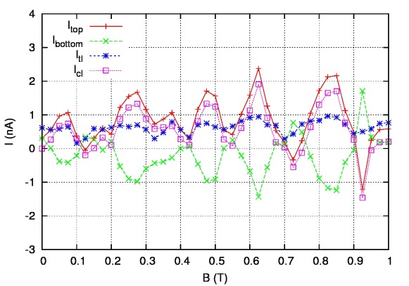
Figure 17: (Color online) Local current through the top ring arm ($I_{\mathrm{top}}$) and bottom ring arm ($I_{\mathrm{bottom}}$) and total local current ($I_{\rm tl}$) and circular local current ($I_{\rm cl}$) versus the magnetic field and averaged over the time interval $[180,220]\mathrm{ps}$ in the case of y-polarized photon field.

In Fig. 17, we show the magnetic field dependence of the local currents $I_{\mathrm{top}}$ and $I_{\mathrm{bottom}}$ through the top and bottom arms, respectively, the total local current $I_{\rm tl}$ across $x=0$, and the circular local current $I_{\rm cl}$. We averaged the local currents over the time interval $[180,220]\mathrm{ps}$ around $t=200$ ps to soften possible high frequency fluctuations (compare with Fig. 13). In most cases (however less often than for x-polarized photons), the top local current exhibits opposite sign to the bottom local current, and hence the circular local current (solid purple) is usually larger than the total local current (dotted blue). The local current through the two current arms, $I_{\rm tl}$, is suppressed in the case of half integer flux quanta showing a similar behavior to the nonlocal currents $I_{L}$ and $I_{R}$ (Fig. 12), but with more irregularities due to the stronger effective influence of the y-polarized photon field. It is interesting to note that the current suppression dip at $B=0.425$ T (marked by the blue arrow in Fig. 12) appears also in the local current (blue dashed curve) flowing through both ring arms from the left to the right.

The circular local current reaches a maximum absolute value of $\max|I_{\rm cl}|=1.905$ nA at $B=0.625$ T, which is by $0.939$ nA smaller than for x-polarization. It is clearly visible from a comparison of Fig. 17 and Fig. 9 that the circular current is considerably smaller than in the x-polarized photon case, while the total local current is of the same order. Thus, the capability of the magnetic field to drive a rotational ring current is weakened by having the electromagnetic field y-polarized. In particular, this can be said about the diamagnetic part of the circular local current leading to the much smaller value $I_{\rm cl}=0.675$ nA at low magnetic field $B=0.05$ T. The periodicity of the circular local current is preserved better for x-polarized photon field as is for the total local current. We note here in passing that it is not possible to understand the non-trivial magnetic field dependence of $I_{\rm cl}$ by resorting solely to a TL description.

IV Concluding Remarks

We have presented a time-convolutionless generalized master equation formalism that allows us to calculate the non-equilibrium transport of Coulomb interacting electrons through a broad quantum ring in a photon cavity under the influence of a uniform perpendicular magnetic field. The topologically nontrivial broad ring geometry allows for substantial electron-electron correlations relative to their kinetic energy and, hence, a large basis is required for sufficient numerical accuracy. The magnetic field, however, increases slightly the energy difference of the 2ES with respect to the 1ES, thus enhancing the 1ES occupation while suppressing the 2ES occupation. The central quantum ring 1ES are charged quickly from both leads. Electron-electron correlation and sequential tunneling slow down the 2ES charging in the long-time response regime. Aharonov-Bohm charge current oscillations can be recognized in the long-time response regime with magnetic field period $B_{0}=\Phi_{0}/A$, which is related to the flux quantum $\Phi_{0}$ and ring area $A$.

In the case of x-polarized photon field, we have found charge oscillations between the left and right part of the quantum ring when the magnetic field is associated with integer flux quanta. The oscillation frequency agrees well with the energy difference of the two mostly occupied states. The relatively high energy difference for x-polarized photons is related to a relatively high transient current through the ring. The amplitude of the charge oscillations through the quantum ring is decreasing in time due to dissipation effects caused by the coupling to the leads. In general, the local current through the upper ring arm exhibits opposite sign to the local current through the lower ring arm. Hence, the “persistent” circular local current is usually larger than the total local charge current through both ring arms from the left to the right. The persistent current shows a periodic behavior with magnetic field, but with a tendency to clockwise rotation due to the contact region vortex structure.

In the case of y-polarized photon field, the magnetic field dependence of the left and right charge current exhibits a pronounced dip at magnetic field $B=0.425$ T corresponding to two flux quanta that is therefore clearly not related to the Aharonov-Bohm effect. The dip is associated with a degeneracy of the two mostly occupied 1ES at magnetic field associated with two flux quanta. The additional level crossing appears only for y-polarized photons. The generally lower energy difference of the two mostly occupied MB states in the case of y-polarization disturbs the constructive phase interference condition for the bias driven charge flow through the quantum device and decreases the persistent current magnitude.

In conclusion, we have demonstrated for our ring geometry that y-polarized photons disturb our system stronger than x-polarized photons, suppressing magnetic field induced currents and perturbing flux periodicity beyond finite width effects by enhancing or suppressing bias-driven currents. It is interesting to compare these findings to the quantum wire case, where it was found that mainly x-polarized photons attenuate the central system charging due to a closer agreement of the photon mode energy and the characteristic electronic excitation energy in x-direction. Gudmundsson et al. (2012) In this paper, we have considered a more complex geometry, which reduces effectively the y-confinement energy $\hbar\Omega_{0}=1.0$ meV. The characteristic electronic excitation energy in y-direction may therefore be much closer to the photon mode energy $\hbar\omega=0.4$ meV, thus leading to a relatively strong influence of the y-polarized photon field on the electronic transport. The conceived magnetic field influenced quantum ring system in a photon cavity could serve as an elementary quantum device for optoelectronic applications and quantum information processing with unique characteristics by controlling the applied magnetic field and the polarization of the photon field.