Spatial Search Algorithms on Hanoi Networks

Abstract

We use the abstract search algorithm and its extension due to Tulsi to analyze a spatial quantum search algorithm that finds a marked vertex in Hanoi networks of degree 4 faster than classical algorithms. We also analyze the effect of using non-Groverian coins that take advantage of the small world structure of the Hanoi networks. We obtain the scaling of the total cost of the algorithm as a function of the number of vertices. We show that Tulsi’s technique plays an important role to speed up the searching algorithm. We can improve the algorithm’s efficiency by choosing a non-Groverian coin if we do not implement Tulsi’s method. Our conclusion is based on numerical implementations.

I Introduction

Grover’s algorithm Gro97a allows one to find a marked item in an unsorted database quadratically faster compared with the best classical algorithm. It is the paradigm for many quantum algorithms that use exhaustive search. The main technique used in Grover’s algorithm, called amplitude amplification, can be applied in many computational problems providing gain in time complexity.

A related problem is to find a marked location in a spatial, physical region. Benioff Ben02 asked how many steps are necessary for a quantum robot to find a marked vertex in a two-dimensional grid with $N$ vertices. In his model, the robot can move from one vertex to an adjacent one spending one time unit. Benioff showed that a direct application of Grover’s algorithm does not provide improvements in the time complexity compared to a classical robot, which is $O(N)$. Using a different technique, called abstract search algorithms, Ambainis et. al. AKR05 showed that it is possible to find the marked vertex with $O\left(\sqrt{N}\log N\right)$ steps. Tulsi Tul08 was able to improve this algorithm obtaining the time complexity $O\left(\sqrt{N\log N}\right)$.

The time needed to find a marked vertex depends on the spatial layout. The abstract search algorithm is a technique that can be applied to any regular graph. It is based on a modification of the standard discrete quantum walk. The coin is the Grover operator for all vertices except for the marked one which is $-I$. The choice of the initial condition is also essential. It must be the uniform superposition of all states of the computational basis of the coin-position space. This technique was applied with success on higher dimensional grids AKR05 , honeycomb networks ADMP10 , regular lattices HT10 and triangular networks ADFP12 . Spatial search in Hanoi network of degree 3 (HN3) was analyzed in Ref. MPB11 . Recently, the abstract search algorithm was applied for spatial search on Sierpinski gasket PR12 .

In this work, we analyze spatial search algorithms on the Hanoi network of degree 4 (HN4) extending the analysis performed for HN3 MPB11 . HN4 is a special case of small world networks, which are being used in many contexts including quantum computing GGS05 ; MPB07 . We also analyze the use of a modified coin operator instead of the Grover coin, which is used in the standard form of the abstract search algorithm, to take advantage of the small world structure. Our results are based on numerical simulations, but the hierarchical structure of HN4 indicates that analytical results can also be obtained. Hanoi networks have a hierarchical structure of fractal type that helps to gain insights of spatial search algorithms in graphs that are not translational invariant. Recently, there has some effort in this direction ABM10 ; PR12

The structure of the paper is as follows. Sec. II introduces the degree-4 Hanoi network. Sec. III describes the standard coined discrete quantum walk on HN4. Sec. IV reviews the basics of the abstract search algorithm and Tulsi’s method. Sec. V describes the modification on the coin operator we propose to enhance the time complexity of quantum search algorithms on HN4. Sec. VI describes the main results based on numerical simulations. Finally, we present our final remarks in Sec. VII.

II Hierarchical Structures

The Hanoi network has a cycle with $N=2^{n}$ vertices as a backbone structure, that is, each vertex is adjacent to 2 neighboring vertices in this structure and extra, long-range edges are introduced with the goal of obtaining a small-world hierarchy. The labels of the vertices $0<k\leq 2^{n}-1$ can be factorized as

$$k=2^{k_{1}}(2\,{k_{2}}+1),$$ (1)

where ${k_{1}}$ denotes the level in the hierarchy and ${k_{2}}$ labels consecutive vertices within each hierarchy. In any level, one links the vertices with consecutive values of ${k_{2}}$ keeping the degree constraint. When ${k_{1}}=0$, the values of $k$ are the odd integers. For HN4, we link 1 to 3, 3 to 5, 5 to 7 and so on. The vertex with label 0, not being covered by Eq. (1), has a loop as well as vertex of label $2^{n-1}$. Fig. 1 shows all edges for HN4 when the number of vertices is $16$. Using this figure, one can easily build HN4 recursively, each time doubling the number of vertices. Our analysis will be performed for a generic value of $n$ to allow us to determine the computational cost as function of $N$.

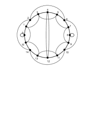
Figure 1: HN4 with 16 vertices.

HN4 has a small-world structure because the diameter of the network only increases with $\sim\sqrt{N}$ BGA08 , less fast than the number of vertices $N$. Yet, HN4 is a regular graph of fixed degree $d=4$ at each vertex.

III Quantum Walks on Hierarchical Structures

A coined quantum walk in HN4 with $N=2^{n}$ vertices has a Hilbert space ${\cal H}={\cal H}_{C}\otimes{\cal H}_{P}$, where ${\cal H}_{C}$ is the $4$-dimensional coin subspace and ${\cal H}_{P}$ the $N$-dimensional position subspace. A basis for ${\cal H}_{C}$ is the set $\{\left|{a}\right\rangle\}$ for $0\leq a\leq 3$ and ${\cal H}_{P}$ is spanned by the set $\{\left|{k}\right\rangle\}$ with, $0\leq k\leq N-1$. We use the decomposition $k=(k_{1},k_{2})$, given by Eq. (1), when convenient. A generic state of the discrete quantum walker in HN4 is

$$\left|{\Psi(t)}\right\rangle=\sum_{a=0}^{3}\sum_{k=0}^{N-1}\psi_{a,k}(t)\left|{a}\right\rangle\left|{k}\right\rangle.$$ (2)

The evolution operator for the standard quantum walk Kem03 is

$$U=S\circ(C\otimes I),$$ (3)

where $I$ is the identity in ${\cal H}_{P}$ and $S$ is the shift operator defined by the following equations,

$$S\left|{0}\right\rangle\left|{k}\right\rangle = \begin{cases}\left|{1}\right\rangle\left|{k_{1},k_{2}+1}\right\rangle,&\mbox{ if }k_{2}\mbox{ is even}\\ \left|{1}\right\rangle\left|{k_{1},k_{2}-1}\right\rangle,&\mbox{ if }k_{2}\mbox{ is odd}\\ \end{cases},$$

$$S\left|{1}\right\rangle\left|{k}\right\rangle = \begin{cases}\left|{0}\right\rangle\left|{k_{1},k_{2}+1}\right\rangle,&\mbox{ if }k_{2}\mbox{ is even}\\ \left|{0}\right\rangle\left|{k_{1},k_{2}-1}\right\rangle,&\mbox{ if }k_{2}\mbox{ is odd}\\ \end{cases},$$

and

$$S\left|{0}\right\rangle\left|{2^{n-1}}\right\rangle = \left|{1}\right\rangle\left|{2^{n-1}}\right\rangle,$$

$$S\left|{1}\right\rangle\left|{2^{n-1}}\right\rangle = \left|{0}\right\rangle\left|{2^{n-1}}\right\rangle,$$

$$S\left|{0}\right\rangle\left|{0}\right\rangle = \left|{1}\right\rangle\left|{0}\right\rangle,$$

$$S\left|{1}\right\rangle\left|{0}\right\rangle = \left|{0}\right\rangle\left|{0}\right\rangle,$$

$$S\left|{2}\right\rangle\left|{k}\right\rangle = \left|{3}\right\rangle\left|{k+1}\right\rangle,$$

$$S\left|{3}\right\rangle\left|{k}\right\rangle = \left|{2}\right\rangle\left|{k-1}\right\rangle.$$

The arithmetical operations on the second ket is performed modulo $N$. The shift operator obeys $S^{2}=I$. $C$ is a unitary coin operation in ${\cal H}_{C}$. In the standard walk, $C$ is the Grover coin, denoted by $G$,

$$G=\frac{1}{2}\begin{pmatrix}-1&1&1&1\\ 1&-1&1&1\\ 1&1&-1&1\\ 1&1&1&-1\end{pmatrix}$$ (4)

which is the most diffusive coin NV00 .

The dynamics of the standard quantum walk is given by

$$\left|{\Psi(t)}\right\rangle=U^{t}\left|{\Psi_{0}}\right\rangle,$$ (5)

where $\left|{\Psi_{0}}\right\rangle$ is the initial condition. After $t$ steps of unitary evolution, we perform a position measurement which yields a probability distribution given by

$$p_{k}=\sum_{a=0}^{2}\left|\left\langle{a,k}\right|U^{t}\left|{\Psi_{0}}\right\rangle\right|^{2}.$$ (6)

IV Abstract Search Algorithms

The abstract search algorithm AKR05 is based on a modified evolution operator $U^{\prime}=S\cdot C^{\prime}$, obtained from the standard quantum walk operator $U$ by replacing the coin operation $C$ with a new unitary operation $C^{\prime}$ which is not restricted to ${\cal H}_{C}$ and acts differently on the searched vertex. The modified coin operator is

$$C^{\prime}=-I\otimes\left|{k_{0}}\right\rangle\left\langle{k_{0}}\right|+C\otimes(I-\left|{k_{0}}\right\rangle\left\langle{k_{0}}\right|),$$ (7)

where $k_{0}$ is the marked vertex in a regular graph and $C$ is the Grover coin $G$, the dimension of which depends on the degree of the graph. Ambainis et. al. AKR05 have shown that the time complexity of the spatial search algorithm can be obtained from the spectral decomposition of the evolution operator $U$ of the unmodified quantum walk, which is usually simpler than that of $U^{\prime}$.

The initial condition $\left|{\psi_{0}}\right\rangle$ is the uniform superposition of all states of the computational basis of the whole Hilbert space. This can be written as the tensor product of the uniform superposition of the computational basis of the coin space with the uniform superposition of the position space. Usually, this initial condition can be obtained in time $O(\sqrt{N})$, where $N$ is the number of vertices.

The evolution operator is applied recursively starting with the initial condition $\left|{\psi_{0}}\right\rangle$. If $t_{f}$ is the running time of the algorithm, the state of the system just before measurement is $U^{\prime t_{f}}\left|{\psi_{0}}\right\rangle$. If one analyzes the probability of obtaining the marked vertex $k_{0}$ as function of time since the beginning of the algorithm, one gets an oscillatory function with the first maximum close to $t_{f}$.

After a little algebra, the evolution operator $U^{\prime}=S\cdot C^{\prime}$ can be converted into the form $U^{\prime}=U\cdot R_{k_{0}}$, where $R_{k_{0}}=I-2\left|{u_{C},k_{0}}\right\rangle\left\langle{u_{C},k_{0}}\right|$, $U$ is given by Eq. (3), and $\left|{u_{C}}\right\rangle$ is the uniform superposition of the computational basis of the coin space. Using the expression $U^{\prime}=U\cdot R_{k_{0}}$ as a starting point, Tulsi proposed a new version of the search algorithm, which requires an extra register (an ancilla qubit) used as a control for the operators $R_{k_{0}}$ and $U$. The operators acting on the ancilla register are described in Figure 2, where $-Z$ is the negative of Pauli’s $Z$ operator and

$$X_{\delta}=\left(\begin{array}[]{cc}\cos\delta&\sin\delta\\ -\sin\delta&\cos\delta\end{array}\right).$$ (8)

The value of $\delta$ is the one that optimize the cost of the algorithm. For two-dimensional lattices, Tulsi Tul08 showed that $\cos\delta\propto 1/\sqrt{\log N}.$

Figure 2: Tulsi’s circuit diagram for the one-step evolution operator of the quantum walk search algorithm. $\left|{u_{P}}\right\rangle$ is the uniform superposition of the computational basis of the position space.

The Tulsi’s evolution operator is

$$U^{\prime\prime}=(-Z\otimes I)\cdot C(U)\cdot(X_{\delta}^{\dagger}\otimes I)\cdot C(R_{k_{0}})\cdot(X_{\delta}\otimes I),$$ (9)

where $C(U)$ and $C(R_{k_{0}})$ are the controlled operations shown in Figure 2 and $I$ is the identity operator in ${\cal H}$. We want to determine how many times $U^{\prime\prime}$ must be iterated, taking $\left|{1}\right\rangle\left|{u_{C}}\right\rangle\left|{u_{P}}\right\rangle$ as the initial condition, in order to maximize the overlap with the search element.

V Modified Method

The coin in a quantum walk is used to determine the direction of the movement. The Grover coin is an isotropic operator regarding all outgoing edges from a vertex. It is useful in networks that have no special directions, such as two-dimensional grids and hypercubes. The Hanoi network, on the other hand, has a special direction that creates the small world structure. Any edge that takes the walker outside the circular backbone provides an interesting opportunity in terms of searching. The strategy is to have a parameter that can control the probability flux among the edges, reinforcing or decreasing the flux outwards or inwards the circular backbone.

Instead of using the Grover coin of the abstract search algorithms, we analyze the use of a modified coin given by

$$\begin{split}C=\frac{2\epsilon}{d}\left(\left|{0}\right\rangle\left\langle{0}\right|+\left|{1}\right\rangle\left\langle{1}\right|+\left|{0}\right\rangle\left\langle{1}\right|+\left|{1}\right\rangle\left\langle{0}\right|\right)+\\ 2\sqrt{\frac{\epsilon(d-2\epsilon)}{d^{2}(d-2)}}\sum_{j=2}^{d-1}\left(\left|{j}\right\rangle\left\langle{0}\right|+\left|{0}\right\rangle\left\langle{j}\right|\right)+\\ 2\sqrt{\frac{\epsilon(d-2\epsilon)}{d^{2}(d-2)}}\sum_{j=2}^{d-1}\left(\left|{j}\right\rangle\left\langle{1}\right|+\left|{1}\right\rangle\left\langle{j}\right|\right)+\\ \frac{2(d-2\epsilon)}{d(d-2)}\sum_{j,j^{\prime}=2}^{d-1}\left(\left|{j}\right\rangle\left\langle{j^{\prime}}\right|\right)-I,\end{split}$$ (10)

where $d=4$ is the degree at each vertex. When $\epsilon=1$, the Grover coin is recovered. When $0<\epsilon<1$, the probability flux along small-world edges (labels 0 and 1) which escapes from the circular backbone is weakened. When $1<\epsilon<4$, the probability flux off the backbone is reinforced, allowing the walker to use the small world structure with higher efficiency. Hence, this new coin controls the bias to escape off the circular backbone of HN4 through the parameters $\epsilon$.

The abstract search algorithms use a uniform distribution as initial condition. We change this recipe. The initial condition is

$$\begin{split}\left|{\psi(0)}\right\rangle=\sqrt{\frac{\epsilon}{d}}\big{(}\left|{0}\right\rangle\left|{s}\right\rangle+\left|{1}\right\rangle\left|{s}\right\rangle\big{)}+\\ \sqrt{\frac{d-2\epsilon}{d(d-2)}}\sum_{j=2}^{d-1}\left|{j}\right\rangle\left|{s}\right\rangle,\end{split}$$ (11)

where $\left|{s}\right\rangle$ is the uniform superposition on the position space. When $\epsilon=1$ the initial condition is the uniform superposition of coin-position space.

We want to check whether it is possible to improve the abstract search algorithm by modifying the coin operator for HN4 in such way we can tune parameter $\epsilon$ for obtaining the best rate of probability flux between the circle backbone and small-world edges. In a previous paper MPB11 , we have concluded that, for HN3 without using Tulsi’s method, it is better to choose $\epsilon=1.75$. After analyzing further this issue, we have to reconsider this conclusion, mainly when one uses Tulsi’s method, which seems to favor the Grover coin even in nonhomogeneous graphs.

In this work, we consider three different methods: 1) the abstract search algorithm, 2) the Tulsi’s method, and 3) the modified method. The analysis of the evolution of the quantum search algorithm using the new coin and initial condition is far more complex than the standard one. Our conclusions here are based in numerical simulations.

VI Main Results

Fig. 3 shows the oscillatory behavior of the probability of finding the walker at the marked vertex using the modified method with $\epsilon=0.75$ (lower curve) and the abstract search algorithm using Tulsi’s method (higher curve). Initially, the probability is close to zero, because the initial condition is a state that is close to the uniform superposition of all vertices. The running time of the algorithm is the value of $t$ for which the probability is close to its first maximum. Note that, without using Tulsi’s method, the maximum value of the probability is smaller than that of the abstract search algorithm with Tulsi’s method. In either case, the maximum value of the probability is not close to 1, as one would expect in order to have high probability to find the marked vertex. This means that the algorithm must be rerun many times to amplify the success probability. For the lower curve, the number of repetitions is large, in fact, it scales with $N$, which has a strong impact on the total cost of the algorithm. We call success probability the value of the probability for the first peak of Fig. 3. The marked vertex used in all simulations is $k=3$, but the conclusions will not depend on the hierarchy of the target vertex.

Figure 3: Probability of finding walker at vertex $k=3$ as a function of time using the modified method and the abstract search algorithm with Tulsi’s method.

Now let us try to answer the following question about parameter $\epsilon$: What is the best value of $\epsilon$ for the spatial search algorithm? Fig. 4 shows the success probability as function of $\epsilon$ for three values of $N$ both for the modified method (lower curves) and the abstract search algorithm using Tulsi’s method (higher curves). The curves are very flat around $\epsilon=1$, which correspond to the Grover coin. This shows the the modified method does not play an important role for improving the efficiency of the algorithm. These curves do not provide enough clues for choosing $\epsilon$. The final answer can be achieved by analyzing the effect of $\epsilon$ on the total cost of the algorithm. We measure the cost as the number of times the evolution operator is applied, or equivalently the number of oracle queries considering the repetitions necessary for amplitude amplification.

Figure 4: Success probability of the search algorithm as function of $\epsilon$ for three values of $N$ using both the modified coin and Tulsi’s method on the top of the abstract search algorithm.

Fig. 5 shows the total cost of the search algorithm as function of $\epsilon$ for two values of $N$ both for the modified method (higher curves) and the abstract search algorithm using Tulsi’s method (lower curves). The curves are very flat around $\epsilon=1$ as before, but we can conclude that the best values are $\epsilon=0.75$ for the modified method and $\epsilon=1$ (Grover coin) for the abstract search algorithm using Tulsi’s method. From now on, we will take these values of $\epsilon$ for the rest of this paper. The fact that the algorithm cannot be improved by modifying the coin after Tulsi’s method seems to show that the algorithm has achieved its best performance using the Grover coin. This conclusion for a graph that has non-homegeneous vertices and non-isotropic edges was not the one expected by us at the beginning and it is quite surprising.

Figure 5: Computational cost of the search algorithm in terms of $\epsilon$ for two values of $N$ using both the modified coin and Tulsi’s method on the top the abstract search algorithm.

Fig. 6 shows the success probability after a single run of the search algorithm as a function of the network size $N$ in log-scale for the modified method (lower points) and the abstract search algorithm using Tulsi’s method (higher points). From the inclination of the best fitting line, we conclude that the success probability of the modified method decays approximately as $0.62/N^{0.37}$. Using the technique of amplitude amplification AKR05 , the algorithm must be rerun around $O(N^{0.185})$ times in order to ensure a final probability close to $1$. This produces a high impact on the total cost of the algorithm. Recall that for the two-dimensional grid, the number of repetitions is $O(\sqrt{\log N})$ AKR05 . This result shows that Tulsi’s method plays an important role in terms of computational complexity. The best value of $\delta$ in Eq. (8) for HN4 seems to be $\cos\delta=O(1/\log N)$. In Fig. 6, we see that success probability after a single run of the abstract search algorithm using Tulsi’s method does not depend on $N$. In this case, we can rerun the algorithm a fixed number of times to obtain an overall probability very close to 1.

Figure 6: Success probability of the search algorithm as a function of $N$. The fitting shows that $P=0.62/N^{0.37}$ for the modified method.

Fig. 7 shows the computational cost of the search algorithm as a function of the network size $N$ both for the modified method (cross points) and the abstract search algorithm using Tulsi’s method (x points). We have not used the method of amplitude amplification in this experiment. We have displayed the best fitting lines for both cases, which scale as $O(N^{0.65})$. For the Tulsi method, this is the total cost of the algorithm, because the success probability is high (see Fig. 6). For the modified method, the total cost is $O(N^{0.84})$, because we must use the method of amplitude amplification, which puts an overhead of $1/\sqrt{P}$, where $P=O(1/N^{0.37})$ (see Fig. 6).

Figure 7: Computational cost of the search algorithm in terms of $N$ in log scale. The dotted curves are fitting curves. For the modified method, the best fitting is $1.25N^{0.65}$. For the Tulsi method, the best fitting is $2.62N^{0.65}$.

It is important to note that the data in Fig. 7 is not precise enough to detect the presence of $\log N$ terms in the expression of the total cost. We are using results with small $N$ to draw conclusions about the asymptotic behavior. There are imprecisions in the simulations that come from the discrete nature of the spatial layout. For instance, the lower curve in Fig. 3 has quick oscillations that have some impact on the impreciseness of the total cost. Usually, the results using Tulsi’s method are more stable.

The scaling of the total cost has a slight variation when we change the position of the target. On the other hand, the prefactor changes. In terms of graph structure, HN4 is non-homogeneous, because the vertices can be divided in hierarchical levels. This non-homogeneity does not play an important role in term of the cost of finding a vertex. The same kind of conclusions holds for HN3, analyzed in Ref. MPB11 .

We have redone and extended the simulations for HN3, using a new implementation. The scaling for the total cost in terms of $N$ is (1) $O(N^{0.62})$ using Tulsi’s method, and (2) $O(N^{0.74})$ using the modified method with $\epsilon=1.75$ applying amplitude amplification. There are two important conclusions we draw from the comparison between HN3 and HN4, one is about the graph degree and the other about the value of $\epsilon$.

The degree of the graph seems to play no important role in terms of efficiency. Similar conclusions were draw in Ref. ADFP12 , which compared the efficiency of quantum search algorithms in triangular, square, and hexagonal lattices that have degrees 3, 4, and 6, respectively. The scaling of the cost as a function of $N$ is the same for all of them.

The optimal value of $\epsilon$ for HN3 is larger than 1 using the modified method, which means that the probability flux toward the edges leaving the circle backbone is enhanced. For HN4, the optimal value of $\epsilon$ is 0.75, smaller than 1. We cannot say that long range connections (in term of hierarchical level) helps in the quantum search. In fact, for HN4 we have to decrease the probability flux in the edges leaving the circle backbone. This can be interpreted, when we take into account that HN4 is really small-world and mean-field like in terms of the average distance between any two vertices, which scales logarithmically with system size, whereas the average distance scales as $\sqrt{N}$ for HN3. That means, in HN4 it is less significant to take long-range jumps, because a random mix is already enough to get to most other sites; whereas in HN3, if the walker does not take more long-range jumps than nearest-neighbor jumps, it is difficult to go very far.

VII Final Remarks

We have analyzed spatial search algorithms on degree-4 Hanoi networks with the goal of extending the abstract-search-algorithm technique for nonhomogeneous graph structures with fractal nature. We have proposed a modification of the abstract search algorithm by choosing a coin that takes advantage of the edge asymmetry of HN4. We have obtained a faster algorithm by tuning numerically parameter $\epsilon$. The cost of this algorithm is $O(N^{0.84})$ in terms of number of oracle queries. The algorithm uses the standard method of amplitude amplification on top of the modified abstract search algorithm with $\epsilon=0.75$. This value of $\epsilon$ tells us that the probability flux is higher on the circle backbone of HN4 than on the edges that produces the small world structure.

We have also analyzed Tulsi’s method on top of the abstract search algorithm. In this case, the Grover coin ($\epsilon=1$) seems to be the best option and the modified method does not improve the algorithm. The cost of the algorithm is $O(N^{0.65})$. This is above the lower bound, which is $O(N^{0.5})$, and above the cost of searching a marked vertex on two-dimensional lattices, which is $O((N\log N)^{0.5})$. We have used numerical methods to estimate the cost scale. This means that $\log N$ factors may be lost, which could decrease the scale of $0.65$ in the total cost.

Our works on progress are now focused on obtaining analytical results regarding search algorithms and general quantum walks for the Hanoi network HN4.

References

- (1) Lov K. Grover. Quantum mechanics helps in searching for a needle in a haystack. Phys. Rev. Lett., 79(2):325–328, Jul 1997.
- (2) Paul Benioff. Space searches with a quantum robot. AMS Contemporaty Math Series, 305, 2002.
- (3) Andris Ambainis, Julia Kempe, and Alexander Rivosh, Coins make quantum walks faster, SODA ’05: Proceedings of the sixteenth annual ACM-SIAM symposium on Discrete algorithms, pp. 1099–1108 (2005).
- (4) A. Tulsi, “Faster quantum-walk algorithm for the two-dimensional spatial search”, Phys. Rev. A 78, 012310 (2008).
- (5) G. Abal, R. Donangelo, F. L. Marquezino, and R. Portugal. Spatial search on a honeycomb network. Mathematical Structures in Computer Science, 20(Special Issue 06):999–1009, 2010.
- (6) Birgit Hein and Gregor Tanner. Quantum search algorithms on a regular lattice. Phys. Rev. A, 82(1):012326, Jul 2010.
- (7) G. Abal, R. Donangelo, M. Forets, and R. Portugal. Spatial quantum search in a triangular network. Mathematical Structures in Computer Science,22:(3):521–531, 2012.
- (8) F.L. Marquezino, R. Portugal, and S. Boettcher. Quantum Search Algorithms on Hierarchical Networks. Information Theory Workshop (ITW), 2011 IEEE, pages 247-251. DOI: 10.1109/ITW.2011.6089429.
- (9) A. Patel and K.S. Raghunthan. Search on a Fractal Lattice using a Quantum Random Walk, arXiv:1203.3950, 2012.
- (10) O. Giraud, B. Georgeot, and D. L. Shepelyansky. Quantum computing of delocalization in small-world networks. Phys. Rev. E, 72(3):036203, Sep 2005.
- (11) Oliver Mülken, Volker Pernice, and Alexander Blumen. Quantum transport on small-world networks: A continuous-time quantum walk approach. Phys. Rev. E, 76(5):051125, Nov 2007.
- (12) E. Agliari, A. Blumen, O. Mülken, Quantum Search on fractal structures, Phys. Rev. A, 82(1):012305 (2010)
- (13) S. Boettcher and B. Gonçalves, “Anomalous diffusion on the Hanoi networks”, EuroPhys. Lett. 84, 30002 (2008).
- (14) J. Kempe, Contemp. Phys. 44, 307 (2003), arXiv:quant-ph/0303081v1.
- (15) A. Nayak and A. Vishwanath. Quantum walk on a line, 2000. DIMACS Technical Report 2000-43, quant-ph/0010117.