date

Giant dielectric permittivity and magneto-capacitance effects in low doped manganites

Abstract

The effect of giant dielectric permittivity due to phase separation accompanied by the charged inhomogeneities in the low doped manganites is discussed. The effect appears in the vicinity of the second order magnetic phase transition which is caused by the long range Coulomb forces. The long range Coulomb interaction is responsible for the formation of the inhomogeneous charged states and determines the characteristic length scales. We derive the phase diagram of the inhomogeneous charged states in the framework of the phenomenological theory of phase transitions. The large value of static dielectric function reduces characteristic value of the Coulomb energy of the inhomogeneous state and makes the appearance of the magnetoelectric effect possible. We discuss the formation of state with giant dielectric permittivity and magneto-capacitance effects in that case.

The importance of the inhomogeneous phase segregated states in the explanation of the anomalous transport and magnetic properties in manganites jin ; tokura ; millis ; nagaev ; dagotto ; dagotto1 ; ramirez ; coey ; kagan1 ; kagan2 and in high temperature superconductors (HTS) gorkov ; emery1 ; grisha is widely discussed. In doped manganites the complex interactions between different degrees of freedom lead to unusual magnetic and transport properties. Moreover it was suggestedmost that spiral magnetic order observed in un-doped manganites $\rm ReMnO_{3}$ may lead to multiferroic behavior. It was also discussed Khoms that the charge ordering in magnetic systems may cause the magnetoelectric effect. Here we propose that the magnetoelectric effect may appear not due to charge ordering but due to charge segregation, which appears near Coulomb frustrated second order phase transition. In this paper we discuss the tendency and conditions of the formation of inhomogeneous states with the spacial charge localization and the phase separation within the phenomenological theory and clarify the role of the Coulomb interaction in this phenomenon. We demonstrate the possibility of the magnetoelectric behavior in the low doped manganites and clarify the role of the Janh-Teller interaction in that behavior.

The problem of Coulomb-frustrated phase separation in different charged systems is the subject of ongoing discussion millis ; nagaev ; dagotto ; dagotto1 ; gorkov ; emery1 ; grisha ; emery3 ; spivak ; jamei ; di_castro_1 ; Lorenz_2 ; mertelj ; fine . Numerous studies have focused on first-order phase transitions where the charge density is coupled linearly to the order parameter (as an external field) jamei ; di_castro_1 or to the square of the order parameter (local temperature) mertelj .

The importance of the Coulomb interaction in the formation of inhomogeneous charged states in the doped manganites was previously emphasized Shenoy_1 ; Shenoy_2 ; Shenoy_3 ; Kugel_jetp ; Kugel_prb2006 ; Kugel_prb2007 . In many cases Shenoy_1 ; Shenoy_2 ; Shenoy_3 ; Kugel_jetp ; Kugel_prb2006 ; Kugel_prb2007 in order to describe the phase separated state near the magnetic phase transition an interaction with additional degrees of freedom were considered. The interaction with these degrees of freedom leads to the energy gain compared to the case of the purely magnetic phase separation. This energy gain is relatively small (about $3kT_{c}\simeq$ 0.03-0.1 eV per one unit cell). Therefore this type of phase separation is not plausible. It follows from the fact that characteristic energy of magnetic interaction $kT_{c}\simeq$ 0.01-0.03 eV is less then the Coulomb energy $V_{c}\simeq$ 0.10-0.13 eV. Here we use the static dielectric constant for manganites $\varepsilon=30-40$. In order to justify the existence of the phase segregation near the magnetic phase transition in the presence of the long-range Coulomb interaction some authorsShenoy_1 ; Shenoy_2 ; Shenoy_3 ; Kugel_jetp ; Kugel_prb2006 ; Kugel_prb2007 underline the important role of the Jahn-Teller effect, which is characterized by the Jahn-Teller energy $J_{JT}$. According to Refs.Shenoy_1 ; Shenoy_2 ; Shenoy_3 ; Kugel_jetp ; Kugel_prb2006 ; Kugel_prb2007 the main contribution to the energy of the low-temperature phase is due to the Jahn-Teller distortions. For example in Refs.Shenoy_1 ; Shenoy_2 the nanoscale electronic inhomogeneities are discussed for $J_{JT}\simeq$ 0.5 eV. In our view in Refs.Shenoy_1 ; Shenoy_2 ; Shenoy_3 the characteristic energy of the Coulomb energy is underestimated $V_{c}\simeq$0.02 eV (for $\varepsilon=20$) at least by the order of magnitude. But what is more important that in manganites the phase separation in the vicinity of the magnetic phase transition is observed. Therefore in order to make correct conclusions about phase separated state we should compare the contribution of the relevant interactions to the total energy of the inhomogeneous state rather then different coupling constants. In this paper we demonstrate that the phase separated state accompanied by the charged inhomogeneities in manganites arises naturally near the magnetic phase transition frustrated by the long range Coulomb forces without coupling with any additional degrees of freedom like Jahn-Teller distortions. We underline that for the existence of this effect it is important to have relatively strong interaction between the electrons and magnetic degrees of freedom. Another important conclusion is that the phase separation becomes plausible due to the self-screening of the space-charge inhomogeneities provided that the screening due to the lattice charges is strong leading to the large values of the dielectric permittivity $\varepsilon$= 30-40. We show that in the absence of the percolation between phase segregated regions there exists a large contribution to the dielectric constant which is connected with the displacements from equilibrium positions of the charged clusters. This contribution to the dielectric function is magnetic field dependent and leads to the magnetoelectric effect. Therefore we expect the giant dielectric permittivity and magnetocapacitance effects in low doped manganites.

We accurately analyze the total energy of the system and treat Coulomb interaction exactly because it is the key factor which determines the characteristics of inhomogeneous states. The idea of phase segregation and inhomogeneous charge distribution in manganites was successfully applied for the description of the magnetoresistive effect in the limit of the percolating charged regions tokura ; millis ; nagaev ; dagotto ; dagotto1 . In this paper we emphasize the possibility of magnetocapacitance effect due to polarization of the non-percolated nano-regions in external electric field in the inhomogeneous state in the low-doped systems.

The phenomenological approach to the theory of Coulomb frustrated phase transition emphasize that the properties the system are universal and are determined by the closeness to the phase transition point and by the dependence of the critical temperature of the phase transition on doping. This approach is essentially independent on other properties of the system. Therefore, the results demonstrate that the properties of the inhomogeneous states are determined by the proximity to the phase transition and the strength of the Coulomb interaction interactions but are independent on other microscopic interactions in manganites.

Our approach indicates that the phase separation with the formation of charged inhomogeneities is a quite common phenomenon inherent to a various systems with the different types of the phase transitions, such as manganites and HTS materials. Our estimates show that the Coulomb energy in the charged separated states is relatively small.

We consider a doped system in the vicinity of a second order magnetic phase transition. We assume that the free carrier density $\rho$ is proportional to the dopant concentration $x=\rho/\rho_{0}$, where $\rho_{0}=e/a^{3}$ characteristic carrier density, $e$ is elementary charge, and $a$ is the lattice parameter. The thermodynamic potential $\Phi=\int\phi(\eta,\rho)d^{3}r$ describes the behavior of the magnetic order parameter $\eta$ near the second order phase transition and the coupling between the order parameter and the charge density reads:

$$\phi(\eta,\rho)=\phi_{0}+\phi_{\eta}+\phi_{int}+\phi_{e}$$ (1)

$$\phi_{\eta}(\eta)=\frac{\alpha}{2}\eta^{2}+\frac{\beta}{4}\eta^{4}+\frac{\xi}{2}(\nabla\eta)^{2}-\eta H$$

$$\phi_{int}(\eta,\rho)=-\frac{\sigma}{2}\eta^{2}\frac{\rho(\rho_{0}-{\rho})}{\rho_{0}^{2}}$$

$${\phi_{e}}(\rho)=\frac{\gamma({\rho(r)}-{\bar{\rho}})}{2\rho_{0}^{2}}\int\frac{({\rho(r^{\prime})}-{\bar{\rho}})}{|r-r^{\prime}|}dV^{\prime}+\frac{\vartheta({\rho(r)}-{\bar{\rho}})^{2}}{2\rho_{0}^{2}}$$

where $\phi_{0}$ is the density of the thermodynamic potential in the high-temperature phase, $\phi_{\eta}$ is the density of the thermodynamic potential of the low-temperature phase, $\alpha$, $\beta$, $\xi$ are coefficients in the expansion of the thermodynamic potentials in powers of the order parameter ($\alpha=\alpha^{{}^{\prime}}(T-T_{c})$, where $T_{c}$ is critical temperature in the absence of doping, $\alpha^{{}^{\prime}}=1/C$, $C$ is the Curie constant), $\xi$ is proportional to the co-called diffusion coefficient of the magnetization $\eta$ and is defined by the exchage ineraction. It defines the characteristic length $\xi^{1/2}$ where the order parameter changes. $H$ is the external magnetic field. $\phi_{int}$ describes the interaction of the order parameter with the charge density, $\sigma$ is the constant of interactions. In order to provide global stability of the system we require $\sigma>0$ emery3 . $\phi_{e}$ describes the charging effects due to Coulomb interaction between the charge carriers, and $\bar{\rho}$ is the average charge density. The spatial distribution of the charge density $\rho$ and the order parameter $\eta$ are determined from minimization of the thermodynamic potential. Therefore the effects of screening are calculated self-consistently during minimization of the thermodynamic potential (1). The inclusion of the gradient term for the charge density is not necessary, because the spatial disribution of the charge density is determined by the minimization of the Coulomb energy. We assume that Coulomb contribution is the strongest: $\vartheta\ll a^{2}\gamma$, where $\vartheta$ is the constant that describes the strength of the local electron-electron interaction, differnt from the Coulomb repulsion. The effect of average dopant concentration $\bar{\rho}$ to the thermodynamic potential in the high-temperature phase is included in $\phi_{0}$. The coefficient $\gamma$ is inversely proportional to the static dielectric constant $\varepsilon$, $\gamma=\rho_{0}^{2}/\varepsilon$. The expression for $\gamma$ takes into account the effect of the local excess positive charge of the lattice explicitly via static dielectric constant. Indeed the direct Coulomb repulsion between electrons in crystals is reduced due to electronic polarizability by the factor $\epsilon_{\infty}$. If we take into account polaronic effects effective interaction between electrons is renormalized and $\epsilon_{\infty}$ should be replaced by the static dielectric function (for details see the Ref. AlexandrovKabanov ). As a result the coefficients in the thermodynamic potential depend on charge density $\rho$ and the term $\sigma\rho(\rho_{0}-\rho)$ determines the shift of the critical temperature $T_{c}$ due to variation of the local charge density:

$$T_{c\rho}(x)=T_{c0}+\frac{\sigma x(1-x)}{\alpha^{{}^{\prime}}}$$ (2)

Here $x=\rho/\rho_{0}$ and $\bar{x}=\bar{\rho}/\rho_{0}$ are dimensionless carrier densities. In the uniform case we have $x=\bar{x}\ (\rho=\bar{\rho})$ and $\eta_{u}=H/2\tilde{\alpha}(\bar{x},T)$ for $T>T_{c0}$ and $\eta_{u}=-\tilde{\alpha}(\bar{x},T)/\beta-H/\tilde{\alpha}(\bar{x},T)$ for $T<T_{c0}$ ($\tilde{\alpha}(x,T)=\alpha(T)-{\sigma}x(1-x)$).

Note that we consider the inhomogeneous states, which appears near the second order phase transition to the ferromagnetic phase. Therefore we do not consider any effect of antiferromagnetic phase or charge ordering. We believe that the influence of the antiferromagnetic or the charge ordered states to the formation of the charge segregated state is not important. We assume that magneto-dipole coupling between bubbles is small in comparison with the exchange interaction. The tunneling of the carriers is important because it leads to the exchange interaction between bubbles. This leads to the magnetic ordering of different bubbles, divergence of the correlation radius and appearance of the macroscopic magnetization in the sample. Therefore we consider the temperature $T_{c\rho}(x_{1})$ (2) as the temperature of the phase transition in the system of bubbles.

In Fig.1 we plot the free energy as a function of the carrier density $x$ for case of the uniform phases. In the region of density where the second derivative of the free energy on $x$ is negative, the uniform state becomes metastable. The phase segregated nonuniform states have lower energy as demonstrated in Fig.1. Therefore there is a tendency to phase separation into domains with different carrier density $x$ (for details see Ref.fine ).

Figure 1: The dependence of the total energy of the uniform state (solid line) on the carrier density $x$. The arrow on the dotted line shows the energy of the phase separated state for case without Coulomb interaction. The arrow on the dashed line indicate the energy of the phase separated state for case where the contribution of the Coulomb interaction is considered. The energy is calculated for the case $\bar{x}=x_{av}$, $T_{c0}=-60K$, $\sigma/\alpha^{{}^{\prime}}=1750K$ for $T=constant$. The parameters $x_{1}$ and $x_{2}$ correspond to the carrier concentrations in the ferromagnetic and in the paramagnetic phases.

In the equilibrium state the order parameter is determined as a steady state solution of the Landau-Khalatnikov equation $\partial\eta/\partial t=\Gamma\delta\phi(\eta,x)/\delta\eta$ Khalatnikov : $\delta\phi(\eta,x)/\delta\eta=0$. The carrier density is determined from the following equation: $\delta\phi(\eta,x)/\delta x=\mu_{e}$, $\mu_{e}$ is the chemical potential, which can be found from the conservation of the total number of carriers. The second equation reads:

$$-\frac{\sigma}{2}\eta^{2}(1-2x(r))+\gamma\int\frac{({x(r^{\prime})}-{\bar{x}})}{|r-r^{\prime}|}dV^{\prime}+\vartheta({x(r)}-{\bar{x}})=0$$ (3)

Using the formula $4\pi\nabla^{2}|r-r^{\prime}|=-\delta(|r-r^{\prime}|)$ and assuming that $\vartheta\ll a^{2}\gamma$, we obtain the dependence of the equilibrium charge density $x_{s}$ on $\eta$:

$$x_{s}(\eta)\simeq\bar{x} - \frac{\sigma(1-2\bar{x})}{8\pi\gamma}\Big{(}{\nabla}^{2}\eta^{2}-\frac{\sigma}{4\pi\gamma}{\nabla}^{2}[\eta^{2}{\nabla}^{2}\eta^{2}]\Big{)}$$

$$- \frac{\vartheta\sigma}{64\pi^{2}\gamma^{2}}\nabla^{4}\eta^{2}$$

Substituting Eq.(4) to Eq.(1) $(\vartheta\ll a^{2}\gamma)$ we obtain the expression of the density of the thermodynamic potential (1) $\phi_{\rho s}$ for the equilibrium distribution of the charge density $x_{s}(\eta)$:

$$\phi_{\rho s}(\eta)=\phi_{\eta}(\eta)-\frac{\sigma\bar{x}(1-\bar{x})}{2}\eta^{2}-\frac{\sigma^{2}(1-2\bar{x})^{2}}{32\pi\gamma}(\nabla\eta^{2})^{2}$$ (5)

$$+\frac{\vartheta\sigma^{2}(1-2\bar{x})^{2}}{256\pi^{2}\gamma^{2}}(\nabla^{2}\eta^{2})^{2}+\frac{\sigma^{3}(1-2\bar{x})^{2}}{128\pi^{2}\gamma^{2}}\eta^{2}(\nabla^{2}\eta^{2})^{2}.$$

The negative sign in the third term of Eq.(5) indicates that the uniform state may be unstable towards inhomogeneous fluctuations.

This instability leads to spatially inhomogeneous solutions. Calculation of the total thermodynamic potential of the inhomogeneous state including the Coulomb energy and the energy interphase boundaries shows that the minimum of the thermodynamic potential corresponds to the phase separated state. Local minima may correspond to different inhomogeneous states where new phase is organized in the form of symmetric bubbles or the periodic stripes or some other arrangements. The most simple solution is spherically symmetric bubbles of the low symmetry phase separated by the large distance from each other.

This type of solution (charged bubble of magnetic phase screened by external charge) represent the minimum of the Coulomb energy together with the energy of the interphase boundaries. Therefore this phase separated state has the lowest energy through the most part of the phase diagram and in particular in the vicinity of the upper boundary of the appearance of the inhomogeneous statesLorenz_2 . Thus this equilibrium inhomogeneous state in the low doped samples has the spherical form and the distribution of charge has a shape of electric double-layer KM_jetf . This solution has characteristic size $R_{0}$. The characteristic average charge density inside of bubbles is $x_{1}$ and the average charge density outside of these regions is $x_{2}$. The average charge density in the system is $\bar{x}$. The average value of the order parameter inside of the bubble $\eta_{1}\simeq\eta_{0}+H/2(-\tilde{\alpha}({x_{1}},T))$ is relatively large, while the order parameter outside of bubbles is much smaller $\eta_{2}=H/\tilde{\alpha}(x_{2},T)$ where $\eta_{0}^{2}=-\tilde{\alpha}({x_{1}},T)/\beta$. It is clear that the charge is concentrated near the surface of the sphere. Therefore we can apply the approximation of the double electrical layer for evaluation of the Coulomb energy. At large distances from the sphere the order parameter and the charge density are equal to their equilibrium values $x=\bar{x}$ and $\eta=\eta_{s}(\bar{x})$ ($\eta_{s}\simeq\eta_{2}(\bar{x})=H/\tilde{\alpha}(\bar{x},T)$). Therefore the thermodynamic potential $\Phi_{s}$ of the volume $V_{0}$ in that case has the form:

$$\Phi_{s}(R_{0},x_{1})=\Phi_{s0}-{A(x_{1})\over{3}}R_{0}^{3}+{B(x_{1})\over{2}}R_{0}^{2}+{C(x_{1})\over{4}}R_{0}^{4},$$ (6)

here $\Phi_{s0}=\phi_{0}V_{0}-{H^{2}V_{0}({2\tilde{\alpha}(x_{2},T)})^{-1}},\ A(x_{1})={\pi\tilde{\alpha}^{2}(x_{1},T)\beta^{-1}}-{2\pi H^{2}\tilde{\alpha}^{-1}(x_{2},T)}+O(H^{3}),\ B(x_{1})\simeq 8\pi\xi d^{-1}\beta^{-1}(-\tilde{\alpha}(x_{1},T)+H\eta_{0}^{-1}(x_{1},T)+H^{2}(4\beta\eta_{0}^{4}(x_{1},T))^{-1}),\ C(x_{1})\simeq\gamma d(\bar{x}-x_{1})^{2}F.$ Here we define dimensionless factor $F$ ($F=4\int\phi_{e}d^{3}r/\gamma R_{0}^{4}d(\bar{x}-x_{1})^{2}$) in order to parameterize the distribution of charge. $F=1/18$ in the limit of the double electrical layer, $V_{0}$ is the volume per one bubble ($V_{0}=V/n$ where $n$ is the number of spheres), $d$ is the interphase boundary thickness. Here we take into account the strong screening of the localized charges and write the Coulomb energy in the double electrical layer approximation. Internal charge of the double electrical layer represents the charge near the surface of the charged bubble. The external charge is of the opposite sign and represents the charge of the region where the density of the charge carriers is reduced. This charge screens the electric field of the charged bubble. As a result the electric field is localized in the vicinity of the charged bubble. This distribution of the electric field directly follows from numerical minimization of the thermodynamic potential (1). In that case it is proportional to $dR_{0}^{4}$. If the screening is absent this energy is proportional to $R_{0}^{5}$ gorkov . The parameters $A(x_{1})$ and $B(x_{1})$ (6) depend on temperature $T$ and magnetic field $H$, and parameter $C(x_{1})$ depends on the average charge density $\bar{x}$. Parameters $(\bar{x},T)$ are external and we find the phase diagram as a function of these parameters. Since $\bar{x}$ is determined by the doping, we describe the evolution of the properties of the system with doping.

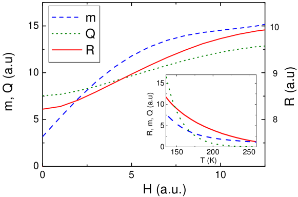
Figure 2: Magnetic field dependence of $R_{s},\ m$ and $Q$. Inset shows the magnetic field dependence of $R_{s},\ m$ and $Q$.

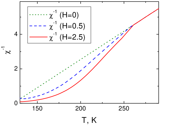
Figure 3: The temperature dependence of $\chi^{-1}(T)$ for two different magnetic fields.

The minimum of the potential $\Phi_{s}(R_{0},x_{1})$ (6) is determined by the set of equations: $\partial\Phi_{s}(R_{0},x_{1})/\partial R_{0}=0$ and $\partial\Phi_{s}(R_{0},x_{1})/\partial x_{1}=0$, which define the equilibrium values of parameters: $R_{s}$ and $x_{1s}$. For the equilibrium size of the charged domain $R_{s}$ we obtain:

$$R_{s}=\displaystyle\frac{y_{\eta}{A_{0}}(x_{1s})-{A}(x_{1s})}{({y(x_{1s})}^{-1}y_{\eta}-1)C(x_{1s})}$$ (7)

And $x_{1s}$ is determined by the equation:

$${\frac{(y_{\eta}{A_{0}}(x_{1s})-{A}(x_{1s}))((y(x_{1s}){A_{0}}(x_{1s})-{A}(x_{1s})}{({y(x_{1s})}^{-1}y_{\eta}-1)(y(x_{1s})y_{\eta}^{-1}-1)B(x_{1s})C(x_{1s})}}=1$$ (8)

where we use the notations: $\eta_{3}=\eta_{0}-{H}{(-\tilde{\alpha}({x_{1}},T))^{-1}},\ {A_{0}}(x_{1})={\pi\tilde{\alpha}^{2}(x_{1},T)\beta^{-1}},\ y(x_{1})={4\sigma(1-2x_{1})(x_{1}-\bar{x})}{(-3\tilde{\alpha}(x_{1},T))^{-1}},\ y_{\eta}={4\eta_{1}}{(3\eta_{3})^{-1}}$ For computer simulation we assume that $x_{2s}\simeq\bar{x}-\lambda(x_{1s}-\bar{x})$. Here $\lambda$ is ratio of the volume of the bubble ($V_{1}$) and the effective volume surrounding the bubble ($V_{2}$), where the charge density $x$ differs from $\bar{x}$. In order to estimate the characteristic length of the phase segregated regions as well as the screening radius it is necessary to perform numerical simulations. Nevertheless some estimates may be performed from Eqs.(7,8). Indeed from Eq.(7) we estimate the typical size of the nano-regions: $R_{0}\simeq 1-5\ nm$. Therefore the distance between bubbles may be estimated as: $L_{R0}\simeq 2(\lambda^{-1/3}-1)R_{0}$ (here $\lambda\sim 0.5$ corresponds to the condition of the compact packing). The thickness of the interphase boundary is equal to the the screening length $d$ should be about $L_{R0}/2$ under the condition of the compact packing.

As a result for the charge of unite bubble $Q$ we have:

$$Q(T,H)=\rho_{0}(x_{1}-\bar{x}){4\pi\over 3}R_{s}^{3}$$ (9)

Average magnetization $m$ is determined by equation:

$$m(T,H)=\eta_{1}\frac{4\pi}{3}\frac{R_{s}^{3}}{V_{0}}+\eta_{2}\Big{(}1-\frac{4\pi}{3}\frac{R_{s}^{3}}{V_{0}}\Big{)}$$ (10)

The temperature and magnetic field dependence of $R(T,H),\ Q(T,H)$ and $m(T,H)$ are shown in Fig.2(a,b). Magnetic susceptibility $\chi(H,T)$ is temperature dependent ($\chi=dm(H)/dH$), as shown in the Fig.3.

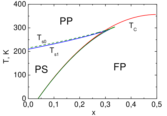
Figure 4: Phase diagram of the system with $T_{c0}=-60K$, $\sigma/\alpha^{{}^{\prime}}=1750K$, $Z=2\ 10^{6}$: $PP$ is the region of the stable high-temperature phase; $FP$ is the region of the stable ferromagnetic low-temperature phase; $PS$ is the region of the stable inhomogeneous phase and metastable homogeneous high-temperature phase.

When the external electric field is applied the charged bubbles shift from equilibrium position. Since the bubbles are not bound to the lattice they will be accelerated by the field. In real systems bubbles will be pinned to the lattice by lattice defects and by the Jahn Teller distortions. Therefore the polarization appears as a result of the shift of the positively charged bubbles with respect to the negative charged background in the case of hole doping. Since the bubbles are not strongly bound to the lattice this shift and the corresponding polarization may be relatively large. Here we assume that this shift will be limited by Jahn-Teller deformation, which bounds the bubbles with the lattice. These arguments may be formulated in terms of relatively simple formula for the effective dielectric constant:

$$\varepsilon_{eff}(T,H)=k\rho_{0}(x_{1}-\bar{x}){4\pi\over 3}R_{s}^{3}$$ (11)

Here $k$ is the coefficient which determines the local lattice deformation which appears due to charge localization and Jahn-Teller effect. Any charge displacement causes additional local deformation of the lattice and therefore protects against large charge displacements. As a result this local Jahn-Teller deformation may be estimated as $d_{JT}(r)\sim k_{JT}\rho_{0}(x(r)-\bar{x})$. In order to take this effect into account we introduce the phenomenological coefficient $k$ in Eq.(11) $k\sim k_{JT}^{-1}$. Note, that in the limit of the strong pinning (for $k_{JT}\to\infty$) the charged bubbles becomes strongly bound to the lattice. Coefficient $k$ in Eq.(11) becomes small leading to the relatively small contribution of bubble displacements to the dielectric permittivity. The value of the coefficient $k$ very difficult to evaluate theoretically. Therefore $k$ should be evaluated from the experiments. But we expect that the pinning is weak. The value of $k$ should be relatively large. The effective dielectric permittivity $\varepsilon_{eff}(T,H)$ (11) is large because of the large value of $k$ and the large value of polarization. Importantly $\varepsilon_{eff}(T,H)$ depends on magnetic field, and therefore has magnetoelectric properties. The coefficient of the magneto-capacitance effect $\Delta\varepsilon/\varepsilon(0)=(\varepsilon(H)-\varepsilon(0))/\varepsilon(0)$ may be estimated from Eqs.(7-11) and Fig.2, where the dependence of the effective charge of the bubbles is plotted as a function of the field. As it follows from Fig. 2 in the magnetic field in the range 5-7T $\Delta\varepsilon/\varepsilon(0)\simeq 0.5-5$. Note, that magnetic field may cause the percolation of the charged regions leading to the strong enhancement of the effect. On the other hand our phenomenological theory is applicable only for the case when different bubbles do not overlap. The discussion of the percolation requires additional theoretical constructions and assumptions and therefore it is out of the scope of our consideration.

The condition that the inhomogeneous phase has lower energy then the uniform state ($\Phi_{s}(R_{0},x_{1})<\Phi_{unif}$) determine the region of the stability of the inhomogeneous phase. The equation $\Phi_{s}(R_{s},x_{1})=\phi_{0}V_{0}-{H^{2}/{2\tilde{\alpha}(\bar{x},T)}}$ define the upper boundary of the existence of the inhomogeneous state. As a result this formula and Eqs.(7,8) define the upper boundary $T_{s1}(\bar{x})$ in the recurrence form as a function of $x_{1}$:

$$T_{s1}=T_{C}+\frac{\sigma}{\alpha^{{}^{\prime}}}x_{1}(1-x_{1})-\frac{\sigma Z}{\alpha^{{}^{\prime}}(1-2x_{1})^{2}}$$ (12)

$$\bar{x}=x_{1}-\frac{2Z}{3(1-2x_{1})^{3}},\ \ \ {\rm where}\ Z=\frac{16\beta\xi\gamma F}{\pi\sigma^{3}}$$ (13)

These equations determine the transition temperature $T_{s1}$ to the stable inhomogeneous phase as a function of external parameters $\bar{x}$. This condition means that the energy of this inhomogeneous phase is lower then the energy of homogeneous state. Applying similar procedure we obtain the equation which defines the lower boundary of the inhomogeneous phase $T_{s2}(\bar{x})$. Note that lower boundary $T_{s2}$ will be always close to the temperature $T_{c\rho}(\bar{x})$, because there is no any gain in energy, when the bubble of the high-temperature phase is formed ($\Phi_{\eta}(\eta=0)=0$, and $\Phi_{\eta}(\eta_{0})<0$). It leads to the essential difference between the formation of the bubble of the low-temperature phase surrounded by the high-temperature phase and the bubble of the high-temperature phase surrounded by the low- temperature phase. The first one is energetically favorable and therefore the region of the existence of these bubbles is considerably large. It is important to note that Eqs.(11) which determine the phase diagram does not depend on $d$. This fact allows us to avoid optimization of the thermodynamic potential with respect to $d$. Typical phase diagram of the inhomogeneous state is presented in Fig.4. Phase transition to the nonhomogeneous state represents typical first order phase transition. Metastable inhomogeneous phase appears at the temperature $T_{s0}$ which is much higher then the temperature of phase transition and it is shown in the phase diagram by dashed line. This line is determined by Eqs.(7,8) and $A(x_{0})^{2}=4C(x_{0},\bar{x})B(x_{0},\bar{x})$. Phase transition from the phase separated state to a FM phase takes place because the thermodynamic potential of the FM phase becomes lower than the thermodynamic potential of the phase separated state. The FM phase becomes the ground states. Moreover below this temperature the phase separated state does not exist. The minimum of the thermodynamic potential corresponding to inhomogeneous state does not exist any longer. Therefore this phase transition is the phase transition of the first order with the characteristic hysteresis.

Let us compare the calculated phase diagram with the experimental phase diagram of $\rm La_{1-x}Sr_{x}MnO_{3}$ muhin . The phase transition at $T_{s}$ corresponds to the transition to inhomogeneous state with the formation of the magnetic long range order at $T_{c}$ muhin . Then with the lowering the temperature the size of bubbles increases and at $T_{c}$ ($T_{p}$ in muhin ) the uniform magnetic state is formed. Note that experimental situation is more complicated. In $\rm La_{1-x}Sr_{x}MnO_{3}$ compound at the temperature $T_{O^{\prime}O^{\prime\prime}}$, which corresponds to the transition from weak to strong distorted Jahn-Teller orthorhombic phase, emerges inhomogeneous fluctuating state. The long-range order between different bubbles is absent in this state. The consideration of this state is out of the scope of our model and therefore it is absent in our phase diagram. Nevertheless we expect that in this state the dielectric permittivity will be large and magnetoelectric effect will be observable as well mamin .

In order to make the phase separation possible it is sufficient to have only small variation of the charge density per unite cell in comparison with average charge density $e(x_{1}-\bar{x})\simeq 0.1-0.2e$. We can estimate the Coulomb contribution to the free energy $u_{\rho}$ as well as the energy gain due to formation of the low-temperature phase $u_{\eta}$ (the forth and the second terms in Eq.(6)) per one unite cell. For the Coulomb contribution we obtain:

$$u_{\rho}=\Bigl{(}{3e^{2}(x_{1}-\bar{x})^{2}\over{4\pi\varepsilon a}}\Bigr{)}{dR_{0}F\over{a^{2}}}$$ (14)

Substituting $\varepsilon=30-40$ (the case of manganites), $F\simeq 1/18$, $R_{0}\simeq 1-5\ nm(d\sim R_{0}),$ to Eq.(14) we obtain that $u_{\rho}$ is less then $0.02eV$. Note that because of the screening the Coulomb energy is strongly reduced and phase separation becomes possible. The energy gain due to formation of the low-temperature phase is $u_{\eta}\simeq 3k_{B}T_{c}$ ($u_{\eta}\simeq a^{3}(\tilde{\alpha}(x_{1},T=0))^{2}/\beta\simeq a^{3}T_{C}\eta_{0}^{2}(x_{1},T=0)/C$, $C=\eta_{0}^{2}(T=0)/3k_{B}N_{A}$, where $N_{A}$ is the Avogadro number). Therefore $u_{\eta}\simeq 0.03-0.1eV>u_{\rho}$ and the phase separation becomes favorable. Therefore the typical size of the nano-regions, which was estimated from Eq.(7) as $R_{0}\simeq 1-5\ nm$, represents quite good approximation.

The analysis of the pair distribution function obtained by neutron scattering shows that the charge density in manganites is localized on the scale of 3 to 4 interatomic distancesdagotto ; louca . The extra charge in that case is not more then $0.1-0.2e$ per unite cell. This is consistent with our estimates. This state is characterized as the state with nano-dimensional charge and phase separation. Dynamics of these charged nano-regions may lead to high value of the effective dielectric constant $\varepsilon_{eff}(T,H)$ (11) in the low frequency range mamin .

We have shown that the second order phase transition with strong dependence of critical temperature $T_{c\rho}(x)$ (2) on doping is unstable with respect to the formation of the spatially inhomogeneous charged states. Within the phenomenological Landau theory we have shown that these states appears at some temperature $T_{s1}$, which is substantially higher then the temperature $T_{c\rho}$ (Fig.4). As a result the phase transition becomes effectively first order phase transition. Note that the Coulomb interaction determines the charge distribution, the screening and the characteristic length scale of the nonhomogeneous states. The spatially inhomogeneous state becomes possible in the systems with the large dielectric constants and with relatively small charge density variations. We demonstrated that the effective dielectric permittivity $\varepsilon_{eff}(T,H)$ (11) is large because of the large value of polarization associated with the shift of bubbles. And the effective dielectric permittivity $\varepsilon_{eff}(T,H)$ depends on magnetic field.

In conclusion we underline that the localized charged states and the phase separation appears even in the case of the second order phase transition. Properties of these states are described within the phenomenological theory of the phase transitions. The Coulomb interaction determines the spatial charge distribution, the screening and the characteristic length of charge localization. The inhomogeneous states become possible because of large dielectric constants and relatively small spatial variation of the charge density. These states in the low doped manganites may lead to the magnetoelectric behavior. The giant value of effective dielectric permittivity and the magneto-capacitance effect in the inhomogeneous state in low-doped systems may become a powerful tool in the investigation of the inhomogeneous charge segregated states in different materials including low-doped cuprates near the threshold the superconducting state.

Enlightening discussions with A.P. Levanyuk, B.Z. Malkin, and D. Mihailovic are highly appreciated. We acknowledge financial support from Slovenian Ministry for Science and Technology and Ad-Futura (Slovenia).

References

- (1) S. Jinet. al., Science, 264, 413 (1994).
- (2) Y.Tokura and N. Nagaosa, Science 288, 462 (2000).
- (3) A.J. Millis et. al., Phys. Rev. Lett. 54, 5144 (1995).
- (4) E.L. Nagaev, Phys. Rev. B60, R6984 (1999).
- (5) E.Dagotto et. al., Physics Reports 344,1 (2001)
- (6) E. Dagotto, New Journal of Physics, 7, 1 (2005).
- (7) A.P. Ramirez, J. Phys. Cond. Mat. 9, 8171 (1997).
- (8) J.M.D. Coey, M. Viret, S. von Molnar, Adv. Phys. 48, 167 (1999).
- (9) M.Yu. Kagan, D.I. Khomskii, M.V. Mostovoy, Eur. Phys. J. B 12, 217 (1999).
- (10) M.Yu. Kagan, K.I. Kugel, Sov. Phys. Uspekhi 44, 553 (2001).
- (11) L.P. Gorkov, J. Supercond., 14, 365, (2001).
- (12) V.J. Emery et. al., Phys. Rev. B56, 6120 (1997).
- (13) L.P. Gorkov and G.B. Teitelbaum, Phys. Rev. Lett. 97, 247003 (2006).
- (14) S.W. Cheong and M. Mostovoy, Nature Materials, 6, 13 (2007).
- (15) J. Van den Brink and D.I. Khomskii J. Phys. Cond. Matt., 20, 1 (2008).
- (16) O. Zachar et. al., Phys. Rev. B57 1422 (1998).
- (17) B. Spivak, Phys. Rev. B67, 125205 (2003); B. Spivak and S.A. Kivelson, Phys. Rev. B70, 155114 (2004).
- (18) R. Jamei et. al., Phys. Rev. Lett. 94, 056805 (2005).
- (19) J. Lorenzanaet. al., Phys. Rev. B, 64, 235127 (2001); C Ortix et. al., Phys. Rev. B, 75, 195107 (2007).
- (20) C. Ortix, J. Lorenzana and C. Di Castro. Phys. Rev. Lett. 100, 246402 (2008).
- (21) T. Mertelj et. al., Phys. Rev. B 76, 054523 (2007); J. Miranda, V.V. Kabanov, Physica C, 468, 358 (2008).
- (22) B. Fine and T. Egami, Phys. Rev. B 77, 014519 (2008).
- (23) Vijay B. Shenoy, et al. Phys. Rev. Lett. 98, 097201 (2007)
- (24) Vijay B. Shenoy, et al. Phys. Rev. B 80, 125121 (2009)
- (25) Vijay B. Shenoy, and C. N. R. Rao. Philosophical Transactions of the Royal Society A: Mathematical, Physical and Engineering Sciences 366, 63 (2008).
- (26) K.I. Kugel et. al., JETP, 98, 572 (2004).
- (27) A.O. Sboichakov et. al., Phys. Rev. B 74, 014401 (2007).
- (28) A.O. Sboichakov et. al., Phys. Rev. B 76, 195113 (2007).
- (29) A.S. Alexandrov, V.V. Kabanov, JETP Lett. 72, 569 (2000).
- (30) L.D. Landau and M.L. Khalatnikov, Dokladi Academy of Since USSR 96, 469 (1954).
- (31) V.V.Kabanov et. al., JETP, 108, 286 (2009).
- (32) D. Louca et. al., Phys. Rev. B 56, R8475 (1997)
- (33) A. A. Mukhin, V. Yu. Ivanov, V. D. Travkin, S. P. Lebedev, A. Pimenov, A. Loidl, and A. M. Balbashov, JETP Lett. 68, 356 (1998).
- (34) R.F. Mamin et. al., Phys. Rev. B 75, 115129 (2007).