Preferential Attachment in the Interaction between
Dynamically Generated Interdependent Networks

Abstract

We generalize the scale-free network model of Barabàsi and Albert [Science 286, 509 (1999)] by proposing a class of stochastic models for scale-free interdependent networks in which interdependent nodes are not randomly connected but rather are connected via preferential attachment (PA). Each network grows through the continuous addition of new nodes, and new nodes in each network attach preferentially and simultaneously to (a) well-connected nodes within the same network and (b) well-connected nodes in other networks. We present analytic solutions for the power-law exponents as functions of the number of links both between networks and within networks. We show that a cross-clustering coefficient vs. size of network $N$ follows a power law. We illustrate the models using selected examples from the Internet and finance.

Network research is a topic of interest with many applications in physics. For example, in quantum chromodynamics, network models have been used in calculating quark-hadron transition parameters Reeves , and Bose-Einstein condensation has connections with network theory Bianconi . Scale-free behavior has been observed in a huge variety of different networks, ranging from the Internet to biological networks Faloutsos ; Barabasi99 ; Adamic ; Albert00 ; Milo ; Garlaschelli03 ; AlbertRMP ; Colizza ; Onnela ; Liben ; Borgatti ; Plamen12 . With few exceptions Buldyrev10 ; VespignaniN ; ParshaniPNAS ; Gao2011 ; Buld11 ; Shao11 ; Son11 ; GaoNP11 , most network studies have focused on single networks that neither interact with nor depend on other networks AlbertRMP . Recently it was noted ParshaniEPL that port and airport networks interact with each other and that the coupling between these networks is not random but correlated. Our general assumption is that real-life scale-free networks are correlated rather than isolated, and that preferential attachment (PA) and its variants Krapivsky00 ; Dorogovtsev00 ; AlbertPRL00 control not only the dynamics within a network but also the dynamics between different networks. In bank-insurance firm networks, for example, we expect large banks to be more attractive to insurance firms than small banks.

Recently, Ref. Holyst06 investigated the behavior of the Ising model on two connected Barabàsi – Albert networks in which each node of the network has a spin, and $J_{AB}=J_{BA}$ are the coupling constants between spins in different networks. Here we emphasize scale-free interdependent network dynamics rather than the robustness of interacting networks Buldyrev10 ; ParshaniPNAS ; Gao2011 ; Buld11 ; Shao11 ; Son11 ; GaoNP11 . We propose a class of stochastic models for scale-free interdependent networks in which interdependent nodes are not randomly connected but are the result of PA. In our approach PA controls not only the dynamics of each network but also the interaction between different networks. First, we define a coupled Barabàsi-Albert (BA) model I composed of two interdependent networks BA₁ and BA₂ where the PA between different networks and within a network is identical. Second, we define a coupled BA model II where the PAs between different networks and within a network are distinct. Third, we define a “network of networks” model. Finally, we present two examples of interdependent networks, from the Internet and from finance.

There are many interdependent networks or “networks of networks” (NON) in real-world data Gao2011 . For example, in physiology, the human body is an example of a NON system that includes the respiratory, nervous, and cardiovascular systems.

As an example of a NON we consider the Internet: a network of routers or autonomous systems (AS) connected by links BarabasiPNAS02 ; Shavitt . Using the fractal concept in which each part of a complex system is an approximate reduced-size copy of the whole—i.e., is “self-similar”—we analyze AS connections not for the entire world BarabasiPNAS02 ; Shavitt but rather the Internet connections between three countries. Specifically, we study AS connections between the US, Germany, and the UK recorded over an 18-month period. For each of the three countries we study both total connectivity ($k^{T}$) and the number of links ($k$) within each country.

In the following analyses, in order to estimate power-law exponent $\gamma$ for a power-law distributed variable $k$ with $P(k)\propto k^{-\gamma}$ we apply two methods. In the Zipf ranking approach in which $R$ denotes rank, one commonly applies the regression

$$\log(\mathrm{k})=a-\zeta~{}\log(R),$$ (1)

where $\zeta=1/(\gamma-1)$, which is strongly biased in small samples Newman05 ; Newman09 ; Gabaix11 . In the first method, in order to overcome this bias, we apply a recently-proposed regression method Gabaix11

$$\log(\mathrm{R}-1/2)=a-(\hat{\gamma}-1)~{}\log(k).$$ (2)

In the second method we estimate the power-law exponent $\hat{\gamma}^{\prime}$ using the equation

$$\hat{\gamma}^{\prime}=1+N[\Sigma_{t=1}^{N}\log(k_{t}/k_{\rm min})]^{-1},$$ (3)

where $k_{\rm min}$ is the smallest value of $k_{t}$ for which the power-law behavior holds, and the sum runs only over those values of $k_{t}$ that exceed $k_{\rm min}$ Newman05 ; Newman09 . Equation (3) is equivalent to the well-known Hill estimator where the standard error on $\hat{\gamma}$, which is derived from the width of the likelihood maximum, is $\sigma=\frac{\gamma^{\prime}-1}{\sqrt{n}}+O(1/n)$.

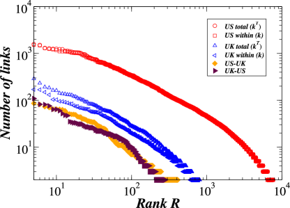
For the sake of simplicity, Fig. 1 shows the NON results of our study on network of routers for only two interdependent countries, the US and the UK. We find that 9685 cities in the US and 1170 cities in the UK are connected by routers. For each country we show (a) the number of links established within the country, (b) the total number of links established not only within the country but also with the coupled country, and (c) the cross links, e.g., the links established from the UK routers to the US routers, and vice versa. Note that no cross-links between UK and the US router networks implies no interdependency between the networks. We find that each Zipf plot of $k$ in Eq. 1 exhibits an approximate power-law scaling. For each country we find that $\hat{\gamma}^{T}$ obtained for total connectivity is smaller than $\hat{\gamma}$ obtained for links within a single country—employing Eqs. (2)–(3) for the US we find $\hat{\gamma}^{T}=2.24\pm 0.01~{}(\hat{\gamma}^{\prime T}=2.17\pm 0.04)$ and $\hat{\gamma}=2.26\pm 0.01~{}(\hat{\gamma}^{\prime}=2.17\pm 0.04)$. For the UK we find $\hat{\gamma}^{T}=2.0\pm 0.01~{}(\hat{\gamma}^{\prime T}=2.21\pm 0.11)$ and $\hat{\gamma}=2.06\pm 0.01~{}(\hat{\gamma}^{\prime}=2.20\pm 0.11)$. We note that similar results for the exponents of degree distributions do not imply that interdependency exists between two networks. To this end, for the cross-links which quantify the level of interdependency between countries (again, no interdependency, no cross-links), we find for US-UK $\hat{\gamma}=2.04\pm 0.03~{}(\hat{\gamma}^{\prime}=1.98\pm 0.09)$ and for UK-US $\hat{\gamma}=2.39\pm 0.02~{}(\hat{\gamma}^{\prime}=2.54\pm 0.24)$. We also show the cross-link interdependent router connections between the UK and Germany, with 1170 cities in the UK and 1989 cities in the Germany. We find for Germany-UK $\hat{\gamma}=2.01\pm 0.03~{}(\hat{\gamma}^{\prime}=2.01\pm 0.15)$ and for UK-Germany $\hat{\gamma}=2.51\pm 0.05~{}(\hat{\gamma}^{\prime}=2.20\pm 0.25)$. Note that the similar degree distributions shown in Fig. 1 never guarantee similar mechanisms of network generations or even other characteristics of networks such as community structures and degree assortativity Boccaletti .

To quantify the level of interdependency between two networks, we next define the cross-clustering coefficient $C_{ij}$ for two scale-free interdependent networks, each with $N$ nodes. Following the definition of the clustering coefficient for a single network Watts , we define the cross-clustering coefficient to be

$$C_{ij}={\cal N}_{ij}/k_{i}\tilde{k}_{j},$$ (4)

where $k_{i}$ and $\tilde{k}_{j}$ are the number of neighbors that nodes $i$ and $j$ have within its own network, and ${\cal N}$ the number of links between the nodes comprising $k_{i}$ and $\tilde{k}_{i}$. For the previous example of the Internet considering, e.g., the two interdependent couples (UK-Germany), chosen because the network size for each country is comparable, we find $\langle C_{ij}\rangle=0.155$. Note that for two independent BA networks, $C_{ij}$ is zero.

For the sake of simplicity we first model a NON system with only two interdependent networks. In model I, each of the two interdependent networks BA₁ and BA₂ begins with a small number ($m_{0}$) of nodes. At each time step $t$, we create a new BA₁ node $j$ with (i) $m_{1}(\leq m_{0}$) edges that link the new node $j$ to $m_{1}$ already existing nodes in BA₁, and with (ii) $m_{12}$ edges that link $j$ to $m_{12}$ already existing nodes in BA₂. We assume that nodes in BA₁ and BA₂ linked to $j$ are chosen based on a version of preferential attachment—the probability $\Pi$ that a new node $j$ in BA₁ is connected to node $i$ in BA₁ depends on the total number of links of node $i$ with the already existing BA₁ and BA₂ nodes (total connectivity). Similarly, the same probability $\Pi$ controls whether a new node $j$ in BA₁ is connected to node $i^{\prime}$ in BA₂.

We define the growth of the BA₂ network similarly. At each time step $t$ we add to the BA₂ network a new node $j^{\prime}$ with $m_{2}(\leq m_{0}$) edges that link $j^{\prime}$ preferentially to $m_{2}$ different nodes already present in BA₂ and with $m_{21}$ links that link $j^{\prime}$ preferentially to $m_{21}$ already existing nodes in BA₁. To reduce the number of parameters we set $m_{21}=m_{12}$. Note that if $m_{21}=0$, while $m_{12}\neq 0$, then due to $m_{21}=0$ each node in BA₁ has an equal number of links $(m_{12})$ to nodes in BA₂, which is unlikely in real-world networks. After $t$ time steps, the four parameters of model I—$m_{1}$, $m_{2}$, $m_{12}$, and $m_{21}$—lead to an interdependent network system with $t+m_{0}$ nodes in both BA₁ and BA₂. BA₁ has the average degree $\langle k\rangle=2m_{1}+m_{12}+m_{21}$ and BA₂ has $\langle k\rangle=2m_{2}+m_{12}+m_{21}$. We perform numerical simulations in which $m_{21}=m_{12}$. We then calculate the probability $P(k)$ that a node in BA₁ has $k$ edges either with BA₁ or BA₂ nodes. We set $m_{1}=m_{2}=3$, and vary $m_{12}=m_{12}$.

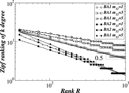
Figure 2 shows that, when $m_{21}=1$, the Zipf plot of $k$ exhibits a power law for varying values of $m_{12}$. With increasing $m_{12}$, $\zeta$ of the Zipf plot decreases ($\gamma$ of $P(k)$ increases), and the $\gamma$ exponent for BA₂ decreases. When $m_{12}=0$, BA₁ and BA₂ become decoupled and yield $(\gamma=3)$, which is characteristic of the BA model. Thus the power-law exponent $\gamma$ of $P(k)$ is a function of the number of links $m_{1}$, $m_{2}$, and $m_{12}(m_{21})$ and, due to interdependencies, $\gamma$ can change substantially for different networks.

Next, for model I we present analytic solutions for the power-law exponent $\gamma$ of $P(k)$ as a function of the number of links both between and within networks. We apply the continuum approach introduced in Refs. Albert00 ; AlbertRMP , which calculates the time dependence of the degree of a given node $i$, e.g., for BA₁. $k^{T}_{1,i}$ is the total number of edges between $i$ in BA₁ and other nodes in BA₁—$k_{1,i}$—and between $i$ and nodes in BA₂—$k_{21,i}$,

$$k^{T}_{1,i}=k_{1,i}+k_{21,i}.$$ (5)

The probability that a new node $j$ created in BA₁ will link to an already existing node $i$ in BA₁ depends on the probability of this process, $\Pi(k^{T}_{1,i})$. Approximating $k^{T}_{1,i}$ with a continuous real variable AlbertRMP , the rate at which $k^{T}_{1,i}$ changes we expect to be proportional to $\Pi(k^{T}_{1,i})$ where

$$\frac{\partial k^{T}_{1,i}}{\partial t}=(m_{1}+m_{21})\Pi(k^{T}_{1,i})=\frac{(m_{1}+m_{21})k^{T}_{1,i}}{2m_{1}t+m_{12}t+m_{21}t}.$$ (6)

¿From the denominator in the last expression we note that each endpoint of an $m_{1}$ edge is a node in BA₁ because $m_{1}$ edges are established between nodes in BA₁. This is in contrast to $m_{21}(m_{12})$ edges where one end is linked to a node in BA₁ and the other to a node in BA₂. The initial condition is that every new node $i$ must have a degree $k^{T}_{1,i}(t_{i})=m_{1}+m_{12}$, since it connects to $m_{1}$ nodes in BA₁ and $m_{12}$ in BA₂. From Eq. (6), we obtain

$$k^{T}_{1,i}(t) = (m_{1}+m_{12})({t}/{t_{i}})^{\beta_{1}},\mathrm{~{}where}$$

$$\beta_{1} = \frac{m_{1}+m_{21}}{2m_{1}+m_{12}+m_{21}}.$$ (7)

Note that in the limiting case $m_{12}=m_{21}=0$ the networks decouple with $\beta=1/2$, as in the BA model Barabasi99 ; AlbertRMP . Other choices for $\beta$ in single networks are proposed in different models Krapivsky00 ; Dorogovtsev00 ; AlbertPRL00 .

The probability that a node $i$ has a degree $k^{T}_{1,i}(t_{i})$ smaller than $k^{T}$ is Albert00 ; AlbertRMP

$$P[k^{T}_{1,i}(t)<k^{T}]=P\left[t_{i}>\frac{(m_{1}+m_{12})^{1/\beta_{1}}t}{(k^{T})^{1/\beta_{1}}}\right].$$ (8)

Assuming that new nodes are entered homogeneously in time, the distribution of $t_{i}$ values is $P(t_{i})=1/(m_{0}+t)$. Entering this expression into Eq. (8) we obtain $P(t_{i}>\frac{\big{(}m_{1}+m_{12}\big{)}^{1/\beta_{1}}t}{(k^{T})^{1/\beta_{1}}})=1-\frac{(m_{1}+m_{12})^{1/\beta_{1}}t}{(k^{T})^{1/\beta_{1}}(t+m_{0})},$ and the degree distribution $P(k^{T})$ of BA₁

$$P(k^{T})=\frac{\partial P(k_{1,i}<k^{T})}{\partial k^{T}}=\frac{(m_{1}+m_{12})^{1/\beta_{1}}t}{(k^{T})^{1/\beta_{1}+1}(t+m_{0})\beta_{1}},$$ (9)

where, asymptotically, for $t\rightarrow\infty$ (networks with an infinite number of nodes), the above equation yields

$$P(k^{T})\propto(k^{T})^{-\gamma_{1}},{\rm~{}where}~{}~{}~{}~{}\gamma_{1}=\frac{1}{\beta_{1}}+1,$$ (10)

with $\beta_{1}$ defined as in Eq. (7). Similar to Eq. (6), $k^{T}_{2,i}$ is the total number of links for a node $i$ in BA₂, which is the total number of edges between BA₂ node $i$ and other nodes in both BA₁ and BA₂, and satisfies the dynamic equation $\frac{\partial k^{T}_{2,i}}{\partial t}=(m_{2}+m_{12})\Pi(k^{T}_{2,i})=\frac{(m_{2}+m_{12})k_{2,i}}{2m_{2}t+m_{12}t+m_{21}t}.$ Following Eqs. (8)-(9), the degree distribution $P(k)$ in the BA₂ network, $\gamma_{2}$, and $\beta_{2}$ is similar to that in Eqs. (7) and (10) in which 1 is replaced by 2 and vice versa.

Unlike the pure BA model, in which $\beta=1/2$ Barabasi99 ; AlbertRMP , in the coupled BA model we find that the power-law exponent of the degree distribution depends on the number of edges within each network, $m_{1}(m_{2})$, and on the number of edges between the interdependent networks $m_{12}(m_{21})$. Also, in agreement with Fig. 1, when $m_{21}=0$, for each $m_{12}$, $\beta_{1}\leq 0.5$ implies $\gamma_{1}\geq 3$ for $P(k)$, whereas $P(k)$ for BA₂ has $\gamma_{1}\leq 3$.

In addition to the degree distribution for the total number of links $k_{i}^{T}$ of Eq. (7), we next provide an analytic result for the degree distribution for the number of links between nodes within a BA₁ network. Following Eqs. (5) and (6), we obtain $\frac{\partial k_{1,i}}{\partial t}=\frac{m_{1}~{}k^{T}_{1,i}}{2m_{1}t+m_{12}t+m_{21}t}$. Entering Eq. (7) into the previous equation, we obtain $k_{1,i}(t)=\frac{m_{1}(m_{1}+m_{12})}{m_{1}+m_{21}}\big{(}\frac{t}{t_{i}}\big{)}^{\beta_{1}}+\frac{m_{1}(m_{21}-m_{12})}{m_{1}+m_{21}}$. Following Eqs. (8)–(9), the degree distribution $P(k)$ for the total number of links between nodes within network BA₁ scales as $P(k)\propto k^{-\gamma_{1}}$ for $t\rightarrow\infty$. Similarly, we calculate the degree distribution $P(k)$ for the total number of links between different networks and again obtain $P(k)\propto k^{-\gamma_{1}}$ where $k_{21,i}(t)=\frac{m_{21}(m_{1}+m_{12})}{m_{1}+m_{21}}\left(\frac{t}{t_{i}}\right)^{\beta_{1}}+\frac{m_{21}(m_{21}-m_{12})}{m_{1}+m_{21}}$. Thus the scaling exponent for $P(k)$ is the same for links connecting nodes of different networks, $k_{21,i}(t)$, links within a given network, $k_{1,i}(t)$, and for the total number of links, $k_{1,i}^{T}(t)$. In practice, by testing this regularity we can determine whether a given pair of interdependent networks follows model I.

Model I has two interesting limits, (i) when $m_{12}=m_{21}=m^{I}$, $\beta_{1}=\beta_{2}=1/2$, as in the pure BA model, and (ii) when $m_{12}\rightarrow\infty$ nodes of BA₁ establish many more connections with BA₂ than with other nodes in BA₁. This implies that $\beta_{1}\rightarrow 0$, as in Eq. (7), and $\beta_{2}\rightarrow 1$, which yields exponents $\gamma_{1}\rightarrow\infty$ (the Gaussian limit), as in Eq. (10), and $\gamma_{2}\rightarrow 2$ (the Zipf law).

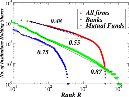
We further exemplify the utility of model I using two networks from Yahoo Finance for 2011. Figure 3 shows 4,544 US firms listed on the NYSE and Nasdaq representing network BA₁, and 15,636 mutual funds representing network BA₂. Note that firms comprising BA₁ and mutual funds comprising BA₂ present only a partial picture of the complete financial network. Clearly, one may extend this analysis by including additional networks such as hedge funds and pension funds. For each firm $i$ of BA₁ we show the total number of holders, i.e., the total number of institutions holding shares (including links from institutional owners such as pension funds, banks, mutual funds, and hedge funds, but also other firms linked to $i$), $k_{1,i}^{T}$. Thus because mutual funds comprising BA₂ hold shares in BA₁, interdependency between the two networks is established. Figure 3 shows the exponents of Eqs. (2)-(3) for US firms: $\hat{\gamma}=2.73\pm 0.01$ ($\hat{\gamma}^{\prime}=3.42\pm 0.17$). For each mutual fund $i$ of BA₂ we show the total number of holdings, which includes firms of BA₁ and also pension funds and other institutions not included in our study. We show the exponents of Eqs. (2)–(3) for mutual funds: $\hat{\gamma}=2.23\pm 0.002$ ($\hat{\gamma}^{\prime}=2.31\pm 0.09$). Figure 3 shows the plot $k^{T}_{1,i}$ vs. rank between rank 20 and 2000. Figure 3 also shows $k^{T}_{1,i}$ vs. rank for US banks, which represent only a small fraction of the total number of US firms, where $\hat{\gamma}=2.17\pm 0.02$ ($\hat{\gamma}^{\prime}=2.39\pm 0.31$). We note that we can replicate these diverse values for $\gamma_{1}$ and $\gamma_{2}$ using model I.

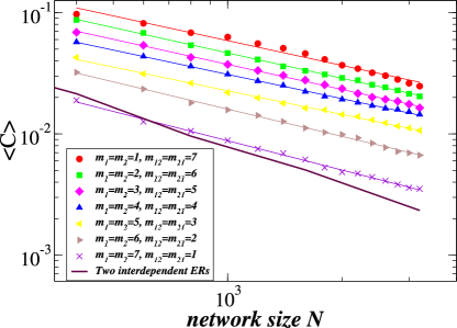
Next we study the scaling of the cross-clustering coefficient $C_{ij}$ of Eq. (4) for two scale-free interdependent networks, each with $N$ nodes, as a function of system size. We study the average of $C_{ij}$ versus $N$, $\langle C\rangle$ versus $N$. To give context to $\langle C\rangle$: in a friendship network $\langle C\rangle$ reflects to what extent an $i$-friend from city A and another $i$-friend from city B know each other. Figure 4 fixes $\langle k\rangle=16$, and varies $m_{1}$, $m_{2}$, and $m_{12}=m_{21}$ in order to numerically determine that $\langle C\rangle$ vs. $N$ follows a power law with an average slope $0.71\pm 0.02$, a value close to $0.75$, which is also obtained numerically for the global cluster coefficient for a single BA network AlbertRMP . As $m_{12}=m_{21}$ increases, the intercept of $\langle C\rangle$ vs. $N$ also increases. Note that for two independent BA networks $\langle C\rangle$ is zero for all $N$. We also study two interdependent Erdos-Renyi (ER) networks, A and B, each of size $N$, where the probability of all links, both between and within networks, is $p$. First we find numerically that $p=0.5\cdot\langle k\rangle/(N-1)$ is needed in order to reproduce a given $\langle k\rangle$ (note that $p=\langle k\rangle/(N-1)$ corresponds to a single ER network). We next find that the cross-clustering coefficient $\langle C\rangle$ vs. $N$ also follows a power law with slope $-1$, the same slope as found for the clustering coefficient vs. $N$ in a single ER model AlbertRMP . Figure 4 shows that the cross-clustering coefficient $\langle C\rangle$ for two interdependent BA models is stronger than $\langle C\rangle$ for two interdependent ER models.

In order to define a new scale-free interdependent network model II in which we separately define the dynamics for growing links within a network and the dynamics for growing links between networks. In model II we create a new BA₁ node $j$ with $m_{1}$ edges that link $j$ to $m_{1}$ existing nodes in BA₁, and with $m_{12}$ edges that link $j$ to $m_{12}$ existing nodes in the BA₂ network at each $t$. Similarly, we link a new node $j^{\prime}$ created in BA₂ with $m_{2}$ edges to $m_{2}$ existing nodes in BA₂. We link new node $j^{\prime}$ to $m_{21}$ existing nodes in BA₁. Links within networks, $k_{1,i}$ and $k_{2,i}$, are treated according to the ordinary scale-free BA model, i.e., using the continuum approach AlbertRMP $\frac{\partial k_{1,i}}{\partial t}=m_{1}\Pi(k_{1,i})=\frac{m_{1}k_{1,i}}{2m_{1}t}$ and $\frac{\partial k_{2,i}}{\partial t}=m_{2}\Pi(k_{2,i})=\frac{m_{2}k_{2,i}}{2m_{2}t}$. Thus links within a network only attract new links created within the same network. We similarly define that only links between networks can attract new links established between networks. The number of links of BA₁ node $i$ with nodes in BA₂, $k_{21,i}$, and the number of links of BA₂ node $i$ with nodes in BA₁,$k_{12,i}$, satisfy $\frac{\partial k_{21,i}}{\partial t}=m_{21}~{}\Pi(k_{21,i})=\frac{m_{21}~{}k_{21,i}}{m_{21}t}$ and $\frac{\partial k_{12,i}}{\partial t}=m_{12}~{}\Pi(k_{12,i})=\frac{m_{12}~{}k_{12,i}}{m_{12}t}.$ Note that in edges $m_{21}(m_{12})$, one end is linked to a node in BA₁ and the other to a node in BA₂. Following Eqs. (6)–(10), we find that the degree distribution $P(k)$ of the number of links between BA₁ and BA₂ becomes $P(k)\propto k^{-\gamma_{3}}$ where $\gamma_{3}=\frac{1}{\beta_{3}}+1$ and $\beta_{3}=1$. This demonstrates that the power-law exponent $\gamma_{3}$ of $P(k)$ does not depend on parameters $m_{1}$, $m_{2}$, $m_{12}$, and $m_{21}$. In addition, $P(k)$ follows a Zipf law. In practice, we can determine whether a pair of interdependent networks follows model II by testing this regularity.

Models I and II, which we have used to study network pairs, can be generalized to $N$ interdependent networks. For each pair $(I,J)$ where $I$ and $J$ run from 1 to $N$, at each time step $t$ we add a new node $j$ to BA_I with $m_{I}$($\leq m_{0}$) edges to $m_{I}$ already existing nodes in BA_I and $m_{IJ}$ edges to $m_{IJ}$ nodes already existing in BA_J. Applying Eqs. (5)–(6), defined for a pair of networks, to the $N$ networks case (the NON model), for $k_{I,i}^{T}$—the total number of edges between a node $i$ and other nodes in BA_I, and between $i$ and other nodes in BA_J—we obtain $\frac{\partial k^{T}_{I,i}}{\partial t}=\frac{(m_{I}+\Sigma_{J=1}^{N}m_{JI})k^{T}_{I,i}}{2m_{I}t+\Sigma_{J=1}^{N}m_{IJ}t+\Sigma_{J=1}^{N}m_{JI}t}.$ Following Eqs. (6)-(10), we find that the degree distribution $P(k)$ of the number of links between BA_I and BA_J becomes $P(k)\propto k^{-\gamma_{5}}$ where $\gamma_{5}=\frac{1}{\beta_{5}}+1$, and $\beta_{5}=(m_{I}+\Sigma_{J=1}^{N}m_{JI})/(2m_{I}+\Sigma_{J=1}^{N}m_{IJ}+\Sigma_{J=1}^{N}m_{JI}).$

Understanding the dynamics of interdependent networks—how different networks simultaneously evolve in time—is a necessary precondition to predicting the behavior of networks over time, and to discovering how quickly failures initiated in one network spread to other networks Schweitzer09 ; Vespignani .

Figure 1: Level of interdependency between countries (no interdependency, no cross-links). Approximate power laws in the Internet obtained for the plot of number of links versus rank $R$ in AS interdependent networks between different countries. We calculate the exponents of Eqs. (2) and (3) for the total number of links and the number of links established only within each country. For the US we obtain $\hat{\gamma}^{T}=2.24\pm 0.01~{}(\hat{\gamma}^{\prime T}=2.17\pm 0.04)$ and $\hat{\gamma}=2.26\pm 0.01~{}(\hat{\gamma}^{\prime}=2.17\pm 0.04)$, and for the UK $\hat{\gamma}^{T}=2.00\pm 0.01~{}(\hat{\gamma}^{\prime T}=2.21\pm 0.11)$ and $\hat{\gamma}=2.06\pm 0.01~{}(\hat{\gamma}^{\prime}=2.20\pm 0.11)$. For the cross-links, we obtain for US-UK $\hat{\gamma}=2.04\pm 0.03~{}(\hat{\gamma}^{\prime}=1.98\pm 0.09)$ and for UK-US $\hat{\gamma}=2.39\pm 0.02~{}(\hat{\gamma}^{\prime}=2.54\pm 0.24)$.

Figure 2: Power law in the plot that a node has $k$ edges, for a model I where $m_{1}=m_{2}=3$, $m_{21}=1$ and $m_{12}$ is varying as 1, 3, and 5. Each network, i.e. BA₁ and BA₂, has 1,000 nodes. The Zipf slope $\zeta$ is inverse of the cumulative distribution exponent $\gamma$, where $\zeta=1/(\gamma-1)$. With increasing $m_{12}$, the Zipf slope $\zeta$ for BA₁ is decreasing $(\gamma$ increasing), whereas the Zipf slope for BA₂ is increasing $(\gamma$ decreasing). We show the case where $m_{12}=m_{21}=0$, $\zeta=0.5~{}(\gamma=3)$, characteristic for the BA model. We show that $P(k)$ is characterized by a power-law exponent that is a function of the number of links $m_{1}$, $m_{2}$, $m_{12}$ and $m_{21}$. With increasing $m_{12}$, for BA₁ we have $\hat{\gamma}_{1}=2.776\pm 0.006$ ($\hat{\gamma}^{\prime}_{1}=3.04\pm 0.20$), $\hat{\gamma}_{3}=3.199\pm 0.007$ ($\hat{\gamma}^{\prime}_{3}=3.32\pm 0.23$) and $\hat{\gamma}_{5}=3.56\pm 0.01$ ($\hat{\gamma}^{\prime}_{5}=3.25\pm 0.22$). With increasing $m_{12}$, for BA₂ we have $\hat{\gamma}_{1}=2.800\pm 0.006$ ($\hat{\gamma}^{\prime}_{1}=3.09\pm 0.20$), $\hat{\gamma}_{3}=2.541\pm 0.005$ ($\hat{\gamma}^{\prime}_{3}=2.66\pm 0.17$) and $\hat{\gamma}_{5}=2.343\pm 0.005$ ($\hat{\gamma}^{\prime}_{5}=2.52\pm 0.15$)

Figure 3: Power laws in interdependent financial networks. Power law in the Zipf plot with exponent $\zeta=(1-\gamma)$ for total number of links versus rank $R$ for $15,636$ mutual funds, $4,544$ US firms and separately for 384 US banks. For each firm $i$ we calculate links from mutual funds and other firms to firm $i$. For each mutual funds $i$ we calculate links from mutual fund $i$ to other mutual funds. We obtain the following exponents: for firms $\hat{\gamma}=2.725\pm 0.008$ ($\hat{\gamma}^{\prime}=3.42\pm 0.17$); for banks $\hat{\gamma}=2.17\pm 0.02$ ($\hat{\gamma}^{\prime}=2.39\pm 0.31$); for mutual funds $\hat{\gamma}=2.231\pm 0.002$ ($\hat{\gamma}^{\prime}=2.31\pm 0.09$).

Figure 4: Power law in the cross-clustering coefficient versus size of the two interdependent Barabaśi-Albert (BA) model with $\langle k\rangle=16$, compared with the cross-clustering coefficient of a random graph, $\approx N^{-1}$. With increasing $m_{12}=m_{21}$ the intercept of power law increases.