Least square based method for obtaining one-particle spectral functions from temperature Green functions

Abstract

A least square based fitting scheme is proposed to extract an optimal one particle spectral function out of any one-particle temperature Green function. It uses the existing non-negative least square(NNLS) fit algorithm to do the fit, and the Tikhonov regularization to help with possible numerical singular behaviors. By flexibly adding delta peaks to represent very sharp features of the target spectrum, this scheme guarantees a global minimization of the fitted residue. The performance of this scheme is manifested with diverse physical examples. The proposed scheme is shown to be comparable in performance to the standard Pade analytic continuation scheme.

An inverse problem tries to make an inference on a cause which is related to a response experimentally accessible by some well-established equation. Usually the relation can be either an integral or a differential equation, which cannot be solved analytically but be treated with utmost numerical careIntroductionToTheTheoryOfInverseProblems . Although being widely involved in different physics fieldsInverse_optical_PhysRevB.73.184507 ; SVD_phonon_fit_PhysRevB.71.104529 ; Baym_JMathPhys.2.232 as well as other areasAnIntroductionToElectromagneticInverseScattering , the inverse problem has largely been an open issue to be fully addressed till now. In this paper, we will focus on a typical inverse problem, the notorious analytic continuation problem, and present a scheme which is comparable to the Pade scheme in their performances.

The analytic continuation problem concerns inferring a spectral function from some input temperature Green function. A temperature Green function, $\mathcal{G}\left(i\omega_{n}\right),$ is related to a one-particle spectral function, $A\left(\Omega\right),$ through an integral equation expressed in Eq. 1 as

$$\mathcal{G}\left(i\omega_{n}\right)=\int_{-\infty}^{\infty}\frac{A\left(\Omega\right)}{i\omega_{n}-\Omega}\frac{d\Omega}{2\pi}$$ (1)

where $\omega_{n}$ can be either fermionic or bosonic Matsubara frequenciesQuanTheOfMBS . Baym and MerminBaym_JMathPhys.2.232 showed unique existence of $A\left(\Omega\right)$ given $\mathcal{G}\left(i\omega_{n}\right)$ at all Matsubara frequency points. Indeed, if the analytic expression is known for $\mathcal{G}\left(i\omega_{n}\right),$ the spectral function can be directly determined via Eq. 2

$$A\left(\omega\right)=-\frac{1}{\pi}\lim_{\eta\rightarrow 0^{+}}\operatorname{Im}\mathcal{G}\left(\omega+i\eta\right)$$ (2)

with the proper analytic continuation to the real axis by replacing $i\omega_{n}$ with $\omega+i\eta$. However, an analytic expression of $\mathcal{G}\left(i\omega_{n}\right)$ is usually not available as it is most often evaluated numerically through Feynmann diagrammatic techniques or other numerical schemesflex_AnnPhys.193.206 ; 1st_QMC_PhysRevB.26.5033 ; QuanTheOfMBS . In these cases, one might have to invert Eq. 1 directly to get an estimation for $A\left(\Omega\right),$ where the unique existence property might be blurred due to numerical errors.

Two types of algorithms are widely used to numerically carry out the analytic continuation depending on different natures of $\mathcal{G}\left(i\omega_{n}\right)$. In case the input data has very high numerical accuracy, the widely used method is the Pade schemeVidberg_JLowTempPhys.29.179 , where the $i\omega_{n}$ dependence of the temperature Green function is approximated with a continued fraction polynomial with higher order expansion terms truncatedEssPadeAppr . By construction, the Pade scheme rigorously reproduces select $\mathcal{G}\left(i\omega_{n}\right)$ points to fulfill the spirit of an analytic continuation. It can give very good results, but sporadically it could also fail by returning negative spectrum or fake sharp peaks in the spectrum. It would thus be ideal if the Pade scheme could be improved free of the above mentioned issues. However, we may argue here that this is not possible. Actually, it is not guaranteed that a valid spectral function is always attainable with an analytic continuation scheme designed to completely reproduce a temperature Green function of finite precision. The logic is the following. Given any temperature Green function, $\mathcal{G},$ we can construct a new temperature Green function, $\mathcal{\tilde{G}},$ defined on a subset of $\mathcal{G}$ as, say,

$$\mathcal{\tilde{G}}\left(i\tilde{\omega}_{n}\right)=\mathcal{G}\left(i\omega_{3n+1}\right)$$ (3)

for $n\in\mathcal{N}.$ $\mathcal{\tilde{G}}$ corresponds to a virtual system whose temperature is increased three times that of the original system in which $\mathcal{G}$ is defined. By construction, $\mathcal{\tilde{G}}$ shares the same spectral function with $\mathcal{G}$, a direct outcome of the theorem by Baym and Mermincomment3_SameSpectr4Gt&G . Now, let’s add an arbitrary perturbation to the $i\omega_{0}$ component of $\mathcal{G}$ and thereby define a second temperature Green function, $\mathcal{G}^{\prime}.$ We immediately see that $\mathcal{G}$ and $\mathcal{G}^{\prime}$ cannot share the same spectral function. Actually there exists no valid spectral function which gives out $\mathcal{G}^{\prime},$ as this spectral function should also give out $\mathcal{\tilde{G}}$ by noting that $\mathcal{\tilde{G}}$ is an infinite size subset of $\mathcal{G}^{\prime}$ as well. On the other hand, however, the Pade type schemes can always be applied to $\mathcal{G}^{\prime}$ and give rise to a ”spectral function”, which cannot be rigorously positive definite as is argued above. We believe that the fact that the Pade scheme is excessively sensitive to numerical round-off errors supports the claim made here.

When the input Green function has a known covariance structure, e.g. data coming from Quantum Monte Carlo simulations1st_QMC_PhysRevB.26.5033 , the analytic continuation has been carried out in a totally different way from the Pade scheme and its alike. Data matching is now not the best thing to do for an analytic continuation due to data error, but instead, models balancing between the input data and the known covariance structure are what people have been looking for. The widely used methods include the Maximum Entropy Method(MEM), the stochastic method and their extensionsJarrell_MEM_PhysRevB.44.5347 ; Sebastian_SA_PhysRevE.81.056701 ; Sandvik_SA_PhysRevB.57.10287 ; Syljuasen_ASM_PhysRevB.78.174429 , where Baysian-type arguments are heavily used. Other methods were tried out as wellearly_QMC_chi2_fit_PhysRevB.34.4744 ; Vitali_GA_PhysRevB.82.174510 ; OptStochReg_Arxiv.cond-mat/0612233v3 . All these research efforts seem to leave one a plausible impression that there is a gap between treating data with or without a known covariance structure when doing an analytic continuation. We believe that this is not necessarily the case if we can find a robust and accurate analytic continuation scheme to treat data with high precision.

Generally speaking, an inverse problem cannot be fully solved numerically unless the input data and the computer system used for the calculation have extremely high precision, as is the case for the analytic continuation problemBeach_PhysRevB.61.5147 . This, together with several practical considerations, suggests some desirable features of a new scheme for doing analytic continuation.

1. The scheme should be robust against numerical round-off errors in the input data.

2. The constraints on the solution should be fully observed to exclude unphysical solutions and to avoid multiple solutions

3. The final solution should be reliable and repeatable, which mainly implies that the scheme has a unique and easily accessible global minimum.

4. The equation establishing the inverse problem should be best preserved when it is transformed into a convenient form for subsequent treatment.

5. Every input data point should be fitted to the statistically highest precision allowed by a computer.

The first point concerns about the scheme as a whole to be practically convenient. The next two points help to render a solution of less arbitrariness. The last two points aim at generating a most accurate solution. The Pade scheme only fulfills conditions (3) and (5). Its sporadic failure suffered from numerical error prevents it from having even wider applications. The Bayesian-type methods don’t seem to satisfy condition (4) and (5) well, thus results coming out of these methods need to be justified by being compared against relevant experiments. We believe that a carefully designed least square fitting scheme can best compromise among the above conditions. There had been some trials with least square based methodsearly_QMC_chi2_fit_PhysRevB.34.4744 ; SVD_spectral_fit_PhysRevLett.75.517 ; Beach_PhysRevB.61.5147 . Former attempts along this line of thought were not carried out carefully enough on approximating the functional formearly_QMC_chi2_fit_PhysRevB.34.4744 ; SVD_spectral_fit_PhysRevLett.75.517 and on preserving nonnegativenessSVD_phonon_fit_PhysRevB.71.104529 of the spectrum. Here we introduce a novel least square based method to fully satisfy all the above mentioned conditions with a slight exception on condition (4).

Very generally, we can assume $A\left(\Omega\right)$ to be parametrized as

$$A\left(\Omega\right)=\tilde{A}\left(\Omega\right)+\sum_{l=1}^{L}I_{l}\delta\left(\Omega-\tilde{\Omega}_{l}\right)$$ (4)

where $\tilde{A}\left(\Omega\right)$ is the continuous part of the spectrum and $\delta\left(\Omega-\tilde{\Omega}_{l}\right)$ represents very sharp quasiparticle peaks which could exist in the system. $I_{l}$ is the spectrum weight of a quasiparticle peak located at $\tilde{\Omega}_{l}$. We usually don’t know the functional form of $\tilde{A}\left(\Omega\right)$. But as a very crude yet later proven to be very efficient step, we approximate $\tilde{A}\left(\Omega\right)$ with joined linear segments within the frequency range of interestcomment1_linear_appr . Denoting $\left\{\Omega_{m}\right\}$ with $m=1,2,\ldots,M$ the pre-chosen frequency grid, and $\left\{A_{m}\right\}$ the unknown magnitudes on the corresponding frequency points, we have

$$\tilde{A}\left(\Omega\right)=\frac{A_{m+1}-A_{m}}{\Omega_{m+1}-\Omega_{m}}\left(\Omega-\Omega_{m}\right)+A_{m}$$ (5)

for $\forall\Omega\in\left[\Omega_{m},\Omega_{m+1}\right].$ If we feed Eq. 5 and Eq. 4 back to Eq. 1 and integrate over each segment, we obtain a linear equation in terms of $A_{i}$ and $I_{i}$,

$$\mathcal{G}\left(i\omega_{n}\right) =\sum_{m=1}^{M-1}\left[\frac{i\omega_{n}-\Omega_{m-1}}{\Omega_{m}-\Omega_{m-1}}\ln\left(\frac{i\omega_{n}-\Omega_{m-1}}{i\omega_{n}-\Omega_{m}}\right)+\frac{\Omega_{m+1}-i\omega_{n}}{\Omega_{m+1}-\Omega_{m}}\ln\left(\frac{i\omega_{n}-\Omega_{m}}{i\omega_{n}-\Omega_{m+1}}\right)\right]A_{m}$$

$$+\sum_{l=1}^{L}\frac{I_{l}}{i\omega_{n}-\tilde{\Omega}_{l}}$$ (6)

Note any integrations incurred in the calculation are carried out analytically. This marks the first difference between our scheme and the previous existing effortsSVD_phonon_fit_PhysRevB.71.104529 ; SVD_spectral_fit_PhysRevLett.75.517 , where discretization error was introduced as the continuous frequency axis was discretized into a frequency grid set up on $\left\{\Omega_{m}\right\}$comment5_PrevLSF . One more relation can be added into Eq. 6 by noticing that $A\left(\Omega\right)$ needs to be normalized to reflect particle conservationcomment2_normal . Meanwhile, the positive definiteness of a spectrum for fermions becomes equivalent to the inequality constraints

$$A_{m},I_{l}\geq 0$$ (7)

under the current construction, which should be rigorously fulfilled. For bosons, the above condition should be slightly modified. Eq. 6, together with the non-negative constraints in Eq. 7, is readily treated by the well-studied non-negative least square fitting algorithm(NNLS)SolvingLeastSquaresProblems if the coefficient matrix formed by the linear coefficients in Eq. 6 is well-behaved, which is however seldomly the case. To resolve this, we resort to the Tikhonov regularization schemeNumericalMethodsforLeastSquaresProblems . The Tikhonov matrix is chosen to be the identity matrix multiplying some cutoff parameter, $\lambda,$ which is set to be about two orders of magnitude higher than the accuracy of the input data, at $10^{-14}$ if not mentioned otherwise in this paper. By doing so, noises are expected to be safely filtered out and only a healthy spectrum is left behind. Note that usually the accuracy of input data is not known a prior. How to reasonably estimate this quantity is suggested in the next paragraph.

In all, given a temperature Green function defined on $N$ Matsbuara frequency points, the Least Square Fitting (LSF) scheme introduced in this paper solves the linear system of equations,

$$\left(\begin{array}[c]{c}\bar{\Phi}\\ \lambda I_{\left(M+L-1\right)\times\left(M+L-1\right)}\end{array}\right)\bar{A}=\left(\begin{array}[c]{c}\bar{\mathcal{G}}\\ \bar{0}_{\left(M+L-1\right)\times 1}\end{array}\right)$$ (8)

for the spectral function. Here, $\bar{\Phi}$ is a $\left(M+L-1\right)\times N$ matrix with the matrix elements defined through Eq. 6 as

$$\bar{\Phi}_{m,n}=\left\{\begin{array}[c]{cc}\dfrac{i\omega_{n}-\Omega_{m-1}}{\Omega_{m}-\Omega_{m-1}}\ln\left(\dfrac{i\omega_{n}-\Omega_{m-1}}{i\omega_{n}-\Omega_{m}}\right)+\dfrac{\Omega_{m+1}-i\omega_{n}}{\Omega_{m+1}-\Omega_{m}}\ln\left(\dfrac{i\omega_{n}-\Omega_{m}}{i\omega_{n}-\Omega_{m+1}}\right)&\text{if }m\leq M-1\\ \dfrac{1}{i\omega_{n}-\tilde{\Omega}_{m-\left(M-1\right)}}&\text{if }m>M-1\end{array}\right.$$ (9)

$\bar{A}$ is the unknown spectral magnitudes defined as

$$\bar{A}_{m}=\left\{\begin{array}[c]{cc}A_{m}&\text{if }m\leq M-1\\ I_{m-\left(M-1\right)}&\text{if }m>M-1\end{array}\right.$$ (10)

and $\bar{\mathcal{G}},$ the input temperature Green function, is simply defined as

$$\bar{\mathcal{G}}_{n}=\mathcal{G}\left(i\omega_{n}\right)$$ (11)

As is usually defined, $I_{\left(M+L-1\right)\times\left(M+L-1\right)}$ and $\bar{0}_{\left(M+L-1\right)\times 1}$ denote an identity matrix and a zero vector respectively.

A crucial piece is missing from the above formalism, that is, we still don’t know how to determine the number and location of quasiparticle peaks to be included in the fit if a continuous spectrum alone cannot give a successful fit to the input Green function. Note that the residue,

$$res=\left\|\bar{\mathcal{G}}-\bar{\Phi}\bar{A}\right\|$$ (12)

returned by Eq. 8, seems to be ”screened” by the continuous spectrum, as is illustrated in Fig 1. This shows that the residue is not sensitive to the location of a tentative delta peak unless it is very close to a true one.

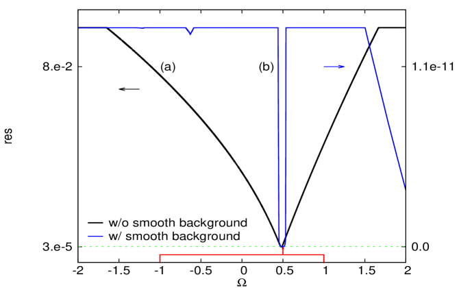
Figure 1: Running residue defined as difference between a fitted and an input Green function for a model system, which has a flat spectrum with a delta peak located around $\Omega\approx 0.5,$ as illustrated in red at the bottom. Curve (a) is calculated by scanning the whole frequency range with just one delta peak, while curve (b) is calculated with a delta peak as well as a continuous background spectrum $\tilde{A}\left(\Omega\right).$ The x axis denotes the scanning position of the delta peak. The y axis denotes the residue defined in Eq. 12 when the scanning delta peak reaches a specific frequency $\Omega$. Note that in the plot the two residues are scaled to be comparable to each other.

To be more specific, we can see that a fit with help of a continuous spectrum gives a very abrupt change in its residue around the true delta peak location, and is much more confined in width than a fit without such a continuous background. The width of the residue drop is approximately $0.09$ when the input data is fitted by a delta peak with a continuous background. This gives the ”highest precision” in determining the location of a delta peak with the current fitting scheme, where any delta peaks within this distance cannot be distinugished. The abrupt drop of residue and its local nature implies two things. Firstly this makes it necessary to carry out a full scan within the interested frequency range to find out all possible quasiparticle locations by checking obvious residue drops, which is not too time-consuming for a one dimensional scan. Secondly, this actually helps the minimization process to reach the global minimum as variables are not strongly dependent on each other any more. If the returned residue is not small enough, one can always repeat the procedure by adding in more peaks until no peaks should be added. Dynamically including more delta peaks into the NNLS fit distinguishes this scheme from all previous trials. As the global minimum can be ensured in this way, the precision of a set of input data can be readily deduced by the best possible fit to the input data with this scheme.

When a fit is to be tested against some known results, the delta peaks need to be transformed such that a direct comparison against the true spectral function is possible. To do that, these delta peaks need to be expanded with help of Eq. 2 as

$$\tilde{I}_{i}\left(\Omega\right)=\frac{1}{\pi}\frac{\eta I_{i}}{\left(\Omega-\Omega_{i}\right)^{2}+\eta^{2}}$$ (13)

We choose $\eta=0.01$ consistently in this work to generate a finite width of a peak and an infinitesmally positive shift to rotate the Green function coming out of the Pade scheme onto the real axis.

The details above outline the general idea on how to carry out the LSF scheme, as illustrated in Fig. 2.

Figure 2: Flow chart of the Least Square Fitting (LSF) scheme. The whole scheme is made up of two loops. The inner loop obtains a best fit to the input Green function for a prefixed error of the input Green function, denoted as res${}_{0}.$ The resulting best fitted error, res, is then used to update res₀ for the outer loop to correct the Tikhonov regularization coefficient $\lambda,$ which controls error propagating from the data to the fitted spectrum in the inner loop. Usually res₀ just needs to be updated once before the whole fit is done.

The portion of the fit with a continuous background is easily implemented, but the portion related to isolated delta peaks becomes very much involved in dealing with various practical concerns, say, how to remove extra tentative peaks added with an intermediate fit, how to push the fit to the extremum of machine precision, etc. After all these issues are carefully addressed, we then look at several examples involving fermions to study the performance of this scheme, using the Pade analytic continuation schemeVidberg_JLowTempPhys.29.179 based on the continued fraction polynomial as a benchmark comparison. For each example, the analytic continuation is carried out with a fit on the lowest $128$ positive Matsubara frequency points for four different temperatures. To make things simpler, we will assume the interested frequency region is known to us. The region is evenly divided to set up the linear system as in Eq. 8, with each interval at least twice the width of a typical residue drop if not mentioned otherwise.

Firstly, two toy model problems are considered whose temperature Green functions are set up through Eq. 1 with artificially constructed spectral functions. The first example considers a step-wise spectral function. We use this example to study the performance of the fitting scheme when a system has a discontinuous spectral function. The second example mimics the Mott-insulating transition under intermediate Hubbard U, which brings up some quasiparticle peaks near the Fermi energy and splits a conduction band into an upper and a lower subbandDMFT_RevModPhys.68.13 . This example mainly stresses on how well the current scheme smoothes through an extremely volatile conduction band, and shows how it could accurately reproduce the delta peaks. With a finite precision for the input data, it is impossible to reproduce every detail of the spectrum in an inverse problem. The cutoff parameter, $\lambda,$ used in the Tikhonov scheme, plays the role of controlling how accurately the true spectrum function can be reproduced.

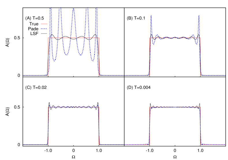
Figure 3: Comparison of the true spectrum function against those returned from the Pade and the LSF schemes for the same step-wise spectrum under different temperatures. For the LSF scheme, evenly divided frequency partition on x axis does not improve fitting quality noticeably beyond a critical number of intervals. It is not very stable for the Pade scheme to work for the current example. Specifically, it requires the number of Matsubara frequency points to be carefully adjusted to get the results shown here.

Fig 3 gives a comparison between the true step-wise spectrum and the Pade analytic continuation results, and the LSF results. The Pade scheme is not very robust in evaluating the spectral function. One needs to carefully choose number of Matsubara frequencies to do the analytic continuation before a reasonable spectrum can be obtained for each temperature. The comparison seems to show that there is a strong temperature dependence on the calculated spectrum with the Pade scheme while the dependence is much weaker with the LSF scheme. It also suggests that both schemes perform better at lower temperature. This is not surprising as reduced $T$ implies denser Matsubara frequency points for an analytic continuation to carry out, thus enabling more information to be used and more features to be extracted out of the original data. The figure does suggest that at a low temperature the LSF scheme is out-performed by the Pade scheme. But one might be cautious in coming up with this conclusion, as quick oscillations could be argued to be an expected feature of a reasonable analytic continuation herecomment4_HighOscillation .

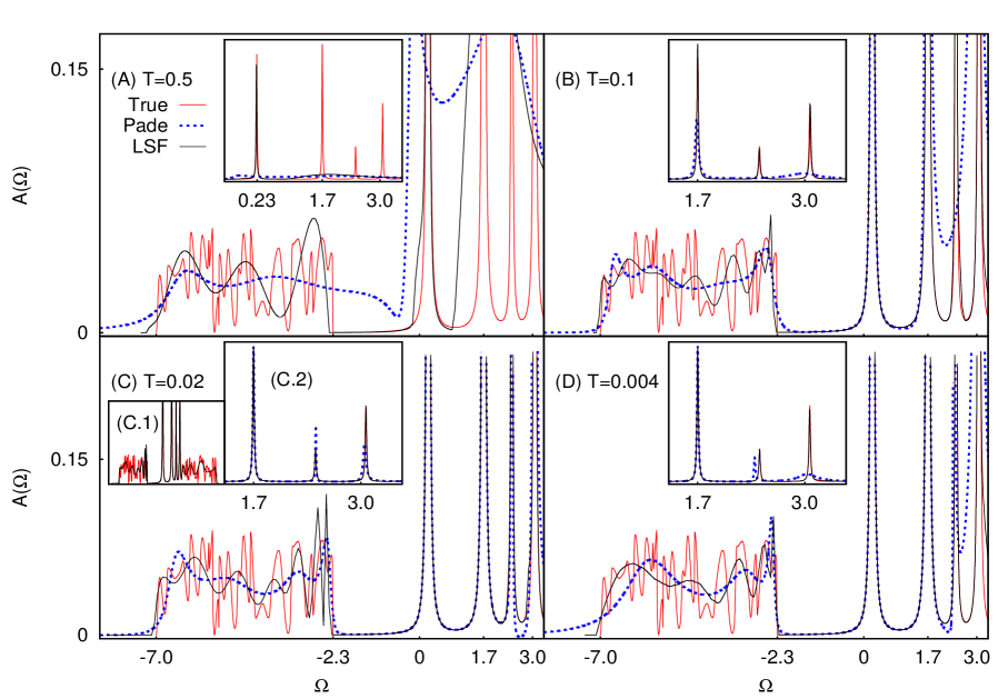
Figure 4: Comparison of the true spectrum composed of two split conduction bands and four delta peaks with results returned from the Pade and the LSF schemes under different temperatures. The overall true spectrum, same for all the four temperature cases, is presented in the left inset of plot (c), together with the corresponding LSF spectrum as a comparison. In each panel, only the lower band and the delta peaks are shown for better data visualization, as the schemes perform alike on both lower and upper bands. With $\eta$ fixed at $0.01$ for consistent comparison, the number of frequency points used in the Pade scheme needs to be chosen carefully for $T=0.1$ and $0.004$ to ensure a valid spectrum function. The inset in each panel presents an overall view of the delta peaks.

Fig 4 presents a comparison between the true spectrum, the Pade analytic continuation results, as well as the LSF results. The true spectrum is made up of two conduction bands and four delta peaks. As can be seen in this specific example, the LSF scheme performs in general better than the Pade scheme for all the temperatures. At $T=0.5,$ the LSF scheme can nearly reproduce the delta peak closest to the zero frequency, but misses the other three peaks which are far away from zero. This is actually a feature of the LSF scheme. It reveals information best around the zero frequency, thus helps to identify the spectrum for low energy excitations around the Fermi level of a physical system. We also see from the plot that the LSF scheme tracks reasonably well the trend of the varying conduction band, which is also an advantage of least square based methods due to their smoothing nature. As the temperature increases, both the Pade and the LSF schemes improve their performance on reproducing the exact spectral function. The performance is better at $T=0.02$ where both schemes are able to reproduce the four delta peaks and track very well the overall trend of the conduction band. But both schemes do less well at $T=0.004,$ and the Pade scheme suffers more. This can be ascribed to the limited number of Matsubara frequencies used for the analytic continuation.

Now let’s look at a more practical problem and see how the current scheme performs on it. To use a relevant model Hamiltonian to describe the physics of the copper-oxide layer of high temperature superconductorsZhang_rice_PhysRevB.37.3759 , we consider the single band repulsive Hubbard model on a square lattice at half filling,

$$H=-t\sum_{\left\langle i,j\right\rangle,\sigma}c_{i,\sigma}^{\dagger}c_{j,\sigma}+U\sum_{i}n_{i,\uparrow}n_{i,\downarrow}$$ (14)

with $\left\langle i,j\right\rangle$ denoting the nearest neighbor hopping. The parameters are chosen at $U=4t$. The bare temperature Green function is defined as

$$\mathcal{G}_{0}\left(i\omega_{n},\mathbf{k}\right)=\frac{1}{i\omega_{n}-\epsilon_{\mathbf{k}}}$$ (15)

where $\epsilon_{\mathbf{k}}=E_{\mathbf{k}}-\mu$ with $E_{\mathbf{k}}=-2t\left(\cos k_{x}+\cos k_{y}\right)$ and $\mu=U/2$ fixed by the particle-hole symmetry to ensure half filling. The second order corrected temperature Green function is calculated asBeach_PhysRevB.61.5147

$$\mathcal{G}\left(i\omega_{n},\mathbf{k}\right) =\frac{1}{\mathcal{G}_{0}^{-1}\left(i\omega_{n},\mathbf{k}\right)-\Sigma\left(i\omega_{n},\mathbf{k}\right)}$$ (16)

$$=\frac{1}{i\omega_{n}-E_{\mathbf{k}}-\Sigma^{\left(2\right)}\left(i\omega_{n},\mathbf{k}\right)}$$ (17)

with

$$\Sigma^{\left(2\right)}\left(i\omega_{n},\mathbf{k}\right)=-\frac{U^{2}}{N^{4}}\sum_{\mathbf{q},\mathbf{k}^{\prime}}\frac{\left[f\left(\epsilon_{\mathbf{k}^{\prime}}\right)+f\left(\epsilon_{\mathbf{q}-\mathbf{k}^{\prime}}\right)-1\right]f\left(\epsilon_{\mathbf{q}-\mathbf{k}}\right)-f\left(\epsilon_{\mathbf{k}^{\prime}}\right)f\left(\epsilon_{\mathbf{q}-\mathbf{k}^{\prime}}\right)}{i\omega_{n}+\epsilon_{\mathbf{q}-\mathbf{k}}-\epsilon_{\mathbf{k}^{\prime}}-\epsilon_{\mathbf{q}-\mathbf{k}^{\prime}}}$$ (18)

Here $f\left(\epsilon_{\mathbf{k}}\right)$ denotes the usual Fermi-Dirac distribution function. For the current study, we are concerned about the spectral function at $\mathbf{k=}\left(0,0\right).$ The true spectrum is obtained by using Eq. 2. The calculation of $\mathcal{G}\left(i\omega_{n},\mathbf{k}\right)$ is performed on a $8\times 8,$ as well as a $100\times 100$ lattice, which would result in different spectrum structures and unknown data errors for analytic continuation schemes to work on.

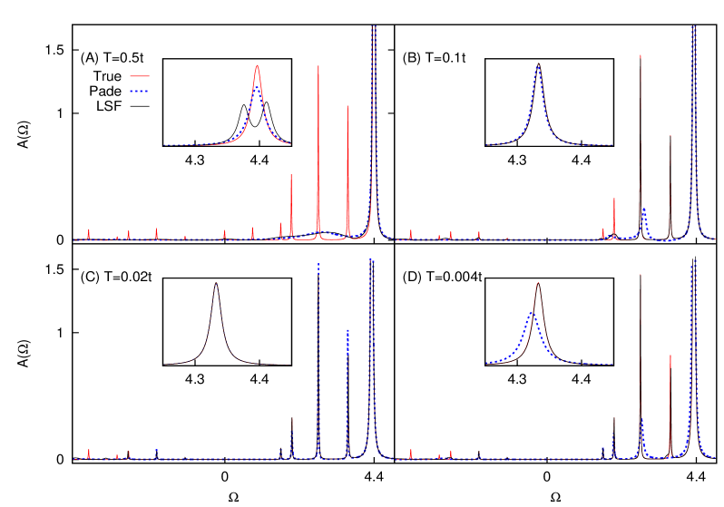
Figure 5: Comparison of the true and the calculated spectral functions using the Pade and the LSF schemes under different temperatures. Pertinent to the half-filled Hubbard model in Eq. 14, the true spectrum is made up of isolated delta peaks, a natural outcome of calculation done on a small (8 by 8) system. In the insets shows the major delta peak around $\omega\approx 4.4$ from different schemes. At $T=0.5t,$ the LSF scheme gives out two delta peaks differring in their locations by about $0.03$, less than the threshold difference of $0.09.$ At $T=0.1t,$ the Pade scheme needs to have the number of Matsubara frequencies adjusted to produce a valid spectral function.

Fig 5 shows a comparison of the true spectrum calculated on a 8 by 8 lattice against the results returned by the two analytic continuation schemes under different temperatures. At $T=0.5t$ in panel A, we see that both schemes perform similarly: only one peak is reproduced well, all the other peaks are generated as a continuum. As shown in the inset, the LSF scheme brings up two delta peaks around $\omega\approx 4.4t,$ which, however, could be an artifact as the peak separation is about $0.03,$ much smaller than the reference width of $0.09$ argued through Fig 1. For the other temperatures, the LSF scheme outperforms the Pade scheme in that it gives very accurate peak locations as well as their intensities. As the temperature is reduced, very much improved fit is obtained, which illustrates once again the importance of denser Matsubara frequencies in producing better results. For the Pade scheme, it performs best at $T=0.02t,$ but still gives wrong intensity of the two delta peaks located around $\omega\approx 3.0t.$ For $T=0.1t,$ the Pade scheme seems to have serious trouble in producing a valid spectral function with $\eta$ fixed at $0.01.$ For $T=0.004t,$ the number of Matsubara frequency points might be too few for a reliable Pade calculation to be carried out, but this does not seem to affect too much the performance of the LSF scheme.

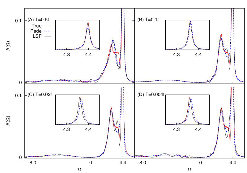
Figure 6: Comparison of the true spectrum of the half-filled Hubbard model on a 100 by 100 lattice against results returned from the Pade and the LSF schemes under different temperatures. As in Fig 5, subtle details of the spectral functions are shown in each plot while presented in each inset is the comparison of the overall behavior of the peak at $\omega\simeq 4.4t$ from each scheme. Due to error cumulation in calculating the input Green function, the best fit achieveable for $T=0.02t$ and $T=0.004t$ can only reach a residue of $10^{-14},$ thus the cutoff parameter $\lambda$ is set at $10^{-12}$ for the calculations of these two cases.

Fig. 6, instead, shows a comparison of the true spectrum on a 100 by 100 lattice against the calculated spectra under different temperatures. For this specific problem, the Pade scheme does a very good job on reproducing the broad continuum at negative energy. But the peak at $\omega\approx 4.4t$ is not reproduced equally well. This is quite different for the LSF scheme, where the major features of the two peaks are reproduced very well, but the continuous spectrum is superimposed with fluctuations. The performance of the LSF scheme is most seriously affected by the fluctuations at either too high or too low temperatures. Further studies are needed to understand why this is the case and to improve the LSF scheme even further. In the current calculation, the data precision of the input Green function is identified to be of $10^{-14}$ for $T=0.02t$ and $T=0.004t.$ Thus the Tikhonov cutoff parameter is set at $\lambda=10^{-12}$ for these two temperatures.

The four examples illustrated above are typical in that they cover cases from having discontinuity, very rapid change, isolated delta peaks and finite data precisions in their spectra. From all these cases, we can see that the performance of the LSF scheme is at least comparable to that of the Pade scheme but with much weaker temperature dependence. It can be well understood that both schemes share comparable performance as they both aim at getting close to $\mathcal{G}\left(i\omega_{n}\right)$ in a best possible way. The only difference is that the LSF scheme preserves the correct $i\omega_{n}$ dependence of $\mathcal{G}\left(i\omega_{n}\right)$ while the Pade scheme approximates $\mathcal{G}\left(i\omega_{n}\right)$ with a continued fraction form. Thus, usually, the LSF scheme gives more accurate extrapolation for $\mathcal{G}\left(i\omega_{n}\right)$ than the Pade scheme if the fitted data are from small Mastubara frequency points. Due to its smoothing nature and limited working precision, the LSF scheme cannot give subtle spectral details but return major features as well as correct trends of hidden data in a systematic and efficient way. Practically, the LSF scheme only uses a very limited number of free parameters, such as, the cutoff parameter pertinant to the Tikhonov regularization, the noise level threshold and the frequency interval to set up the one dimensional frequency grid. The resulting spectrum does not critically depend on these adjustable parameters as long as their values can be reasonably justified.

The current LSF scheme does need further development and testing in several aspects. The most relevant one is what if delta peaks have a finite broading. It is still unknown how efficiently the continuous background spectrum $\tilde{A}\left(\Omega\right)$ is able to pick up this feature. A second concern is in case a delta peak exists within the support of a continuous spectrum. The fitted delta peak will take up some nearby spectral weight which necessarily results in a deformation of the continuous background. One more concern of the current scheme is about the linear approximation of the continuous spectrum. It would be interesting to see how much one can improve if the continuous background spectrum is approximated with a cubic interpolation. All these concerns are either numerically too involved or impossible to address within the current scheme when the frequency grid is set up with evenly divided frequency intervals. We reserved them for future work.

In summary, we have shown that the LSF scheme introduced here has comparable performance aganist the Pade scheme. It is able to systematically uncover major features of the unknown spectral function hidden in $\mathcal{G}\left(i\omega_{n}\right)$. This is made possible by working with a spectral function and a temperature Green function in the frequency space expressed in Eq. 1 where the high frequency information is suppressed only mildly. As a comparison, one might be faced with the difficulty caused by the exponential suppression of a spectral function when the analytic continuation problem is formulated in the imaginary time spaceearly_QMC_chi2_fit_PhysRevB.34.4744 . The analytic continuous problem is a notoriously difficult one to solve. As is well-known, the resulting coefficient matrix for the reformulated linear inverse problem is necessarily ill-conditioned. But, it seems in the current study the Tikhonov regularization fixes this issue pretty well. Meanwhile, dynamically adding delta peaks into the linear inverse problem helps to reach the global minimum of the fitted residue, while using a continuous spectrum background in the fit helps to improve the efficiency in minimization. As the continuous spectrum is able to adapt itself to any broad variation, failure to reach the known global minimum, viz vanishing residue, must be due to sharp features which cannot be captured by the continuous background. This observation underlies the idea how to add tentative delta peaks into the fit. As the whole fitting process is least square based, this necessarily gives out a more robust way to do the analytic continuation than the Pade scheme. Actually we have tried to argue at the very beginning of this paper that the Pade scheme is inherently vulnerable to data errors. So far, the current LSF scheme can only be applied to high precision data. Given further improvement on its performance and robustness, this scheme might be used to treat data from a Quantum Monte Carlo simulation, where the covariance matrix structure is known for the input temperature Green function. Meanwhile, the current scheme might be easily adapted to other inverse problems involving integral equations as well. In addition, it might find much wider applications in both experimental data analysis, say, in neutron scattering and optical measurements, and many engineering fields if its performance can be further enhanced. Future efforts on the inverse problem with the least square fitting scheme will be directed along these dirctions.

The author would like to acknowledge Junyu Guo, Yi Xue and Shina Tan for many useful discussions. He would also like to thank Prof. Kai-Ming Ho and Dr. Cai-Zhuang Wang for insightful discussions and kind help. Research supported by the U.S. Department of Energy, Office of Basic Energy Sciences, Division of Materials Sciences and Engineering. Ames Laboratory is operated for the U.S. Department of Energy by Iowa State University under Contract No. DE-AC02- 07CH11358.

References

- (1) A. L. Bukhgeim, Introduction to the Theory of Inverse Problems (VSP BV, 2000)
- (2) E. Schachinger, D. Neuber, and J. P. Carbotte, Phys. Rev. B 73, 184507 (May 2006)
- (3) S. V. Dordevic, C. C. Homes, J. J. Tu, T. Valla, M. Strongin, P. D. Johnson, G. D. Gu, and D. N. Basov, Phys. Rev. B 71, 104529 (2005)
- (4) G. Baym and D. Mermin, J. Math. Phys. 2, 232 (1961)
- (5) K. I. Hopcraft and P. R. Smith, An Introduction to Electromagnetic Inverse Scattering (Kluwer Academic Publishers, 1992)
- (6) A. L. Fetter and J. D. Walecka, Quantum Theory of Many-Particle Systems (McGraw-Hill Book Company, 1971)
- (7) N. E. Bickers and D. J. Scalapino, Ann. Phys. 193, 206 (1989)
- (8) J. E. Hirsch, R. L. Sugar, D. J. Scalapino, and R. Blankenbecler, Phys. Rev. B 26, 5033 (1982)
- (9) H. J. Vidberg and J. W. Serene, J. Low. Temp. Phys. 29, 179 (1977)
- (10) J. G. A. Baker, Essentials of Pade Approximants (Academic Press, INC., 1975)
- (11) Baym and Mermin’s theorem implies that a unique spectral function exists for a given temperature Green function. Obviously the spectral function giving gives as well. Thus, there exists no other spectral function which gives except for the one derived from .
- (12) M. Jarrell, J. E. Gubernatis, and R. N. Silver, Phys. Rev. B 44, 5347 (1991)
- (13) S. Fuchs, T. Pruschke, and M. Jarrell, Phys. Rev. E 81, 056701 (2010)
- (14) A. W. Sandvik, Phys. Rev. B 57, 10287 (1998)
- (15) O. F. Syljuasen, Phys. Rev. B 78, 174429 (2008)
- (16) H. B. Schüttler and D. J. Scalapino, Phys. Rev. B 34, 4744 (1986)
- (17) E. Vitali, M. Rossi, L. Reatto, and D. E. Galli, Phys. Rev. B 82, 174510 (2010)
- (18) I. S. Krivenko and A. N. Rubtsov, Arxiv.cond-mat/0612233v3(2011)
- (19) K. S. D. Beach, R. J. Gooding, and F. Marsiglio, Phys. Rev. B 61, 5147 (2000)
- (20) C. E. Creffield, E. G. Klepfish, E. R. Pike, and S. Sarkar, Phys. Rev. Lett. 75, 517 (1995)
- (21) This is actually not a terrible approximation if the frequency range of interest is divided into tiny pieces and the continuous part of the spectrum is smooth enough.
- (22) This is a conventional way to approximate an integration. But for an inverse problem, this might introduce excessive unvalidated errors into the problem as the quality of a solution can be very sensitive to errors.
- (23) We didn’t apply the normalization constraint to the current calculation. Actually, this constraint was automatically fulfilled to an extremely high precision by various spectra of different systems coming out of this scheme. This observation gave us additional confidence in this method. Specifically, for relatively high temperatures, the normalization constraint can be fulfilled to as high as the machine accuracy, while for low temperature, the deviation can also reach .
- (24) C. L. Lawson and R. J. Hanson, Solving Least Squares Problems (Prentice-Hall, 1974)
- (25) A. Bjorck, Numerical Methods for Least Squares Problems (SIAM, 1996)
- (26) A. Georges, G. Kotliar, W. Krauth, and M. J. Rozenberg, Rev. Mod. Phys. 68, 13 (1996)
- (27) We can observe this oscillation behavior on the step-wise spectral function example treated by the Pade scheme by gradually increasing data precision. Formally, we can argue it the following way. We apply an inverse Fourier transformation to bring the retarded Green function, , back to the time regime, and we have , with for and vanishing otherwise. One can then solve for and transform back to recover . Numerically however, big error will be introduced for at large as the kernel exponentially decays to zero. This leaves unrealistic high frequency oscillation behaviors in the final expression of . In making the above arguement, please note and are closely related.
- (28) F. C. Zhang and T. M. Rice, Phys. Rev. B 37, 3759 (1988)