An Angle Dependent SSC Model for Relativistic Jet Sources

Abstract

We report on the development of a numerical code to calculate the angle-dependent synchrotron + synchrotron self-Compton radiation from relativistic jet sources with partially ordered magnetic fields and anisotropic particle distributions. Using a multi-zone radiation transfer approach, we can simulate magnetic-field configurations ranging from perfectly ordered (unidirectional) to randomly oriented (tangled). We demonstrate that synchrotron self-Compton model fits to the spectral energy distributions (SEDs) of extragalactic jet sources may be possible with a wide range of magnetic-field values, depending on their orientation with respect to the jet axis and the observer. This is illustrated with the example of a spectral fit to the SED of Mrk 421 from multiwavelength observations in 2006, where acceptable fits are possible with magnetic-field values varying within a range of an order of magnitude for different degrees of B-field alignment and orientation.

1 Introduction

Blazars form one of the most energetically extreme classes of Active galactic nuclei (AGN). Blazars can be observed in all wavelengths, ranging from radio all the way up to $\gamma$-rays. Their spectral energy distribution (SED) is characterized by two broad non-thermal components, one from radio through optical, UV, or even X-rays, and a high-energy component from X-rays to $\gamma$-rays. In addition to spanning across all observable frequencies, blazars are also highly variable across the electromagnetic spectrum, with timescales ranging down to just a few minutes at the highest energies.

There are two fundamentally different approaches to model the SEDs and variability of blazars, generally referred to as leptonic and hadronic models (see, e.g., Böttcher, 2007, for a review of blazar models). In the case of leptonic models, where leptons are the primary source of radiation, synchrotron, synchrotron self-Compton (SSC), and external-Compton (EC) radiation mechanisms are employed to explain the blazar SED (see, e.g., Marscher & Gear, 1985; Maraschi et al., 1992; Dermer et al., 1992; Ghisellini & Madau, 1996). The focus of the present study is also on a leptonic model. In hadronic models, the low-energy SED component is still produced by synchrotron emission from relativistic electrons, while the high-energy component is dominated by the radiative output from ultrarelativistic protons, through photo-pion induced cascades and proton synchrotron emission (e.g., Mannheim & Biermann, 1992; Mücke & Protheroe, 2001; Mücke et al., 2003). One aspect common to all blazar models is a relativistic jet oriented at a small angle with respect to our line of sight, resulting in relativistic Doppler boosting and the shortening of observed variability time scales.

Given computational limitations, the complex physical processes in relativistic jets can, realistically, only be evaluated with certain simplifying approximations. In order to facilitate analytical as well as numerical calculations, the two most common approximations employed in blazar jet models are to assume that the magnetic (B) field is randomly oriented and tangled, and that the lepton momentum distribution is isotropic in the comoving frame of the high-energy emission region. These two assumptions greatly simplify the evaluation of the synchrotron and Compton emission by eliminating various integrals over the interaction and scattering angles. However, there is increasing evidence (Attridge et al., 1999; Lyutikov et al., 2005; Marscher et al., 2008) for a fairly well defined helical B-field structure within AGN jets. These observations also suggest a spine-sheath geometry for AGN jets. The differential velocity profiles within the jet is expected to create anisotropies in the particle distributions. It is therefore important to explore jet models where we can not only simulate an ordered B-field, but also study the resulting radiation behaviour with anisotropic lepton distributions.

1.1 B-Field estimates

The standard approach to diagnosing the magnetic field properties is via synchrotron polarization. If the underlying distribution of emitting electrons is a power-law with power-law index $p$, the maximum degree of synchrotron polarization is given by:

$$\Pi=\frac{P_{\perp}(\nu)-P_{\parallel}(\nu)}{P_{\perp}(\nu)+P_{\parallel}(\nu)}=\frac{p+1}{p+\frac{7}{3}}$$ (1)

where $P_{\perp}(\nu)$ and $P_{\parallel}(\nu)$ are the synchrotron power per unit frequency in directions perpendicular and parallel to the projection of the magnetic field on the plane of the sky. Using equation 1 we can see that for a power-law index of $p=3$, the degree of polarization can be as high as 75%.

It is therefore possible to estimate the magnetic field orientation based on polarization measurements, but an estimate of the field strength usually requires the consideration of flux and spectral properties of the synchrotron emission. Furthermore, polarization measurements are notoriously difficult (and even barely feasible at frequencies higher than optical), and may often not give realistic results due to Faraday rotation and depolarization along the line of sight. In this work, we are interested in taking a complementary approach to estimating the magnetic field orientation where the difference in observed flux levels of the spectrum can give an estimate of how the magnetic orientation may be changing.

Figure 1: The $B_{iso}/B_{\alpha}$ ratio shows how the B-field estimate can vary depending on the electron power-law index and whether one assumes an isotropic B-field or a specific pitch angle.

The principle behind this approach can be demonstrated when one compares the B-field estimates based on a power-law distribution of electrons with an arbitrary power-law index, $p$ , and pitch angle, $\alpha$. The comparison of synchrotron emission coefficients for a power-law distribution of electrons with and without pitch-angle ($\alpha$) dependence gives us a measure of how the estimated magnetic field strength can differ. The emission coefficients can be found in Longair (1994) and are given by (in the units of $\mathrm{erg~{}s^{-1}cm^{-3}Hz^{-1}}$):

$$j_{\alpha}(\nu) = \frac{\sqrt{3}\mathrm{e}^{3}\mathrm{B}\kappa\sin\alpha}{2m_{e}c^{2}(p+1)}\left(\frac{4\pi\nu m_{e}c}{3e\mathrm{B}\sin\alpha}\right)^{-(p-1)/2}$$ (2)

$$\times \Gamma(\frac{p}{4}+\frac{19}{12})\Gamma(\frac{p}{4}-\frac{1}{12})$$

and

$$j_{\mathrm{iso}}(\nu) = \frac{\sqrt{3}\mathrm{e}^{3}\mathrm{B}\kappa}{4m_{e}c^{2}(p+1)}\left(\frac{4\pi\nu m_{e}c}{3e\mathrm{B}}\right)^{-(p-1)/2}$$ (3)

$$\times \frac{\Gamma(\frac{p}{4}+\frac{19}{12})\Gamma(\frac{p}{4}-\frac{1}{12})\Gamma(\frac{p}{4}+\frac{5}{4})}{\Gamma(\frac{p}{4}+\frac{7}{4})}~{}.$$

Where $\kappa$ is the electron distribution power-law normalization. The above two expressions can be solved for the magnetic field to obtain:

$$\frac{B_{\mathrm{iso}}}{B_{\alpha}}=\left(\frac{2}{\sqrt{\pi}}\frac{(\sin\alpha)^{\frac{p-1}{2}}\Gamma(\frac{p}{4}+\frac{7}{4})}{\Gamma(\frac{p}{4}+\frac{5}{4})}\right)^{2/(p+1)}\ .$$ (4)

This gives an estimate of how, for a given luminosity, the B-field estimates can differ depending upon whether we assume an isotropic pitch angle approximation or a given pitch angle (which, in the case of relativistic electrons, is equal to the angle between the magnetic field and the line of sight). The above relation is only applicable in the optically thin regime. We can see in figure 1 that depending on the pitch angle assumption, and the electron distribution power-law index, the $B_{iso}/B_{\alpha}$ fraction can range from 0 (there is negligible synchrotron emission along an ordered magnetic field) to $\sim 1.25$. Because the Compton emissivity is approximately isotropic for an isotropic distribution of electrons, the ratio $F_{SSC}/F_{Sy}$ will change with the pitch angle. It is therefore important to see how the overall synchrotron and synchrotron-self Compton spectra differ with well ordered magnetic fields. One point worth noting is that in our set-up the lower limit on B-field orientation is limited by the $\delta(\Omega_{sy}-\Omega_{e})$ approximation (see section 2.2); a magnetic field perfectly aligned with the observing direction will give zero output. However, in a more rigorous treatment, the lower limit on the minimum angle, $\alpha$, for the B-field orientation will be determined by the relativistic beaming characteristic of synchrotron emission along an electron’s direction of motion into a cone of opening angle $\alpha_{\rm sy}\sim 1/\gamma$, where $\gamma$ is the electron Lorentz factor. In the case of optical frequencies and magnetic fields of $B\sim 1$ G, $\alpha_{min}$ will be the order of $10^{-4}$, while in the X-ray regime $\alpha_{min}\sim 10^{-5}$. Using the relation in equation 4 it is possible to estimate the effects on the B-field estimates between this value of $\alpha_{min}$ and an isotropic magnetic field. For a power-law index of 3, $\alpha_{min}$ gives $B_{iso}/B_{\alpha}$ value of 0.0039.

2 The Model

The following section briefly outlines our model, including the synchrotron radiation and Compton scattering treatments followed as well as the numerical techniques used to implement them.

2.1 Volume, B-field, and Distributions

$\begin{array}[]{c}\includegraphics[width=151.76964pt]{figure2.epsi}\\ \includegraphics[width=151.76964pt]{figure3.epsi}\\ \end{array}$

Figure 2: Top: The electron and B-field interaction angles. Bottom: Cell/Jet geometry illustrating how the photon spectrum can be observed as a function of various angles, $\theta_{cell}$ and $\phi_{cell}$, with respect to the cell. The electron and photon distributions are defined with respect to the cell.

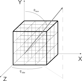
Figure 3: Volume/Jet geometry illustrating how a block of cells can be used to construct a larger volume. $\theta_{view}$, the viewing angle with respect to the volume/jet is incorporated into Doppler boosting calculations.

In our model the basic volume structure is a cubic cell. This allows the model to be modular and build an arbitrarily large volume with any desired anisotropies. Each cell contains a magnetic field plus electron and photon distributions. The magnetic field can have an arbitrary orientation and strength in each cell. This means that the overall volume can be modelled to contain a completely uniform, partially anisotropic, or pseudo-random B-field. The purpose of the present work is to isolate the effects of the degree of order and orientation of the magnetic field on the emerging synchrotron emission. Therefore, we choose the simplest conceivable approach concerning the electron distribution, and do not take electron cooling into account. This means, we only focus on static electron distributions which do not evolve due to energy losses. In future work we aim to include self-consistent cooling effects which would also allow us to probe how the pitch-angle dependence of the synchrotron cooling would give rise to different electron distributions in different cells, depending on the magnetic field set-up.

The directional information in the electron and photon distributions and the B-field is with respect to the cell. In the case of electrons the distribution is a function of energy and two angles with respect to the cell (see figure 2). This gives us the ability to create anisotropies in the electron distributions as well by either having preferential direction for the electrons or by setting up the electron distributions differently in various cells. For both electrons and photons, the distributions’ energy grids (Lorentz factor $\gamma$ for electrons and frequency $\nu$ for the photons) are calculated using logarithmic binning. Therefore each distribution is modelled using a 3 dimensional array with the dimensions of $[\mathrm{bins}_{\gamma/\nu}\times\mathrm{bins}_{\theta}\times\mathrm{bins}_{\phi}]$. Figures 2 (right) illustrates how various angles with respect to the cell are defined. Angles $\theta_{cell}$ and $\phi_{cell}$ run from 0 to $\pi$ and 0 to 2$\pi$ respectively. In figure 3 we can see how the overall volume can be constructed from individual cells. For a given viewing angle, the emission from the visible outer layer of cells is combined to produce an overall spectrum from an effectively larger volume.

The simulation currently transfers, from one cell to another, only the photons. In order to achieve this, we need to calculate which of the six cubic faces a given photon direction will intersect. To calculate this, we assume that all the photons are produced in the center of the cell, and then trace photon paths in any given direction towards the nearest boundary. Even though our simulation considers a static situation, the transfer and radiative feedback between different cells requires an inherent time-dependence in the code. The time step for our radiation transfer approach is the light crossing time across a single cell, which is equal to the time it takes for the photons to travel from one cell to another. At the end of each time step and depending on the physical processes being modelled, the photon distribution is modified and passed to the appropriate neighbour. When being passed to a neighbour the entire photon distribution is passed. Therefore at the end of a time-step each cell’s (intrinsic) photon distribution is emptied into six neighbouring cells, unless it is a boundary cell. The six incoming (transiting) photon distributions are stored until the start of the following time-step when they are combined to form a single intrinsic photon distribution again. The physical processes are then carried out on this single photon distribution. Synchrotron radiation is calculated first and the photons added to the intrinsic distribution. Compton scattering is carried out after the synchrotron radiation. At this point we reach the end of a time-step and the process of transferring photon distributions to neighbouring cells begins again. The observed photon distribution originates from the boundary cells. The photon distributions emerging from visible faces of the boundary cells are combined to create a single observed photon distribution. This process of combining the photon distributions from the boundary cells in effect treats the whole multi-cell structure like a single cubic/cuboid structure.

2.2 Synchrotron radiation

Here we highlight the key points of the synchrotron radiation treatment that we follow. A more in-depth analysis and details can be found in Longair (1994).

The synchrotron emissivity per electron, $P_{\nu}$, is given by:

$$P_{\nu}=\frac{\sqrt{3}e^{3}B\sin\alpha}{m_{e}c^{2}}F(x)~{}~{},$$ (5)

where F(x) is given by:

$$F(x)=x\int_{x}^{\infty}{K_{5/3}(z)\mathrm{d}z}~{}~{}.$$ (6)

$x=\nu/\nu_{c}$, where $\nu_{c}$ is the critical frequency given by $3\gamma^{2}eB\mathrm{sin}\alpha/4\pi m_{e}$c. $\alpha$, the pitch angle, is calculated using spherical trigonometry:

$$\cos(\alpha) = \cos(\theta_{e})\cos(\theta_{B})\$$ (7)

$$+ \sin(\theta_{e})\sin(\theta_{B})\cos(\phi_{B}-\phi_{e})~{}~{}.$$

The synchrotron emission coefficient is given by:

$$j_{\nu}(\Omega_{sy}) = \oint_{4\pi}\mathrm{d}\Omega_{e}\int_{1}^{\infty}\mathrm{d}\gamma n(\gamma,\Omega_{e})$$ (8)

$$\times P_{\nu}~{}\delta(\Omega_{sy}-\Omega_{e})~{}~{}.$$

The numerical Bessel function integration in equation 6 can be time consuming. However, some fast routines to perform this integration are given by Umstätter (1981) which we modified for our precision and computer language.

In a full treatment of the synchrotron radiation the emitted photons are distributed within a solid angle ($\Omega\sim 1/\gamma^{2}$) about the pitch angle $\alpha$. However, for our purposes we assume the emitted photons travel in the same direction as the emitting electrons.

A detailed calculation of synchrotron self-absorption can be found Longair (1994). The absorption coefficient when recast in terms of electron Lorentz factors, $\gamma$, instead of $E$, can be written as:

$$\chi_{\nu}=-\frac{1}{8\pi m\nu^{2}}\int_{1}^{\infty}P_{\nu}\frac{\mathrm{d}}{\mathrm{d}\gamma}\left(\frac{N(\gamma)}{\gamma^{2}}\right)\gamma^{2}\mathrm{d}\gamma~{}~{}.$$ (9)

The photons produced via synchrotron radiation are added to the intrinsic photon distribution of the cell. The photons received from neighbouring cells are added to the intrinsic photon distribution prior to calculating the synchrotron spectrum. Therefore the photons passing through any cell are also synchrotron self-absorbed. The emission and absorption coefficients are used to calculate the total spectrum,

$$I_{\nu}=\frac{j_{\nu}}{4\pi\chi_{\nu}}(1-e^{-\tau_{\nu}})~{}~{},$$ (10)

where $\tau_{\nu}=\chi l$ is the optical depth and l is the size of the emission zone/cell.

2.3 Compton scattering

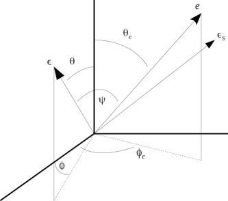
Figure 4: Various angles involved in the Compton scattering of photons with energy $\epsilon$ to $\epsilon_{s}$ off electrons $e$

In the limit $\gamma>>1$, and in the electron rest frame, the incident photon travels in nearly the opposite direction to the electron. This is due to photon aberration:

$$\cos\theta^{\prime}=\frac{\cos\psi-\beta_{e}}{1-\beta_{e}\cos\psi}~{}~{}.$$ (11)

When $\beta_{e}\rightarrow 1$, $\cos\theta^{\prime}\rightarrow-1$, we are in the head-on approximation regime, which we employ to greatly simplify Compton cross section calculations. That is, we can assume that the scattered photon solid angle, $\Omega_{s}$, is well approximated by the electron solid angle $\Omega_{e}$. When the differential Compton (Klein-Nishina) cross section is integrated over $\Omega_{s}$, we get (Dermer & Menon, 2009):

$$\frac{\mathrm{d}\sigma_{C}}{\mathrm{d\epsilon_{s}}}\simeq\frac{\pi r_{e}^{2}}{\gamma\epsilon^{\prime}}\Xi_{C}\mathrm{H}\left(\epsilon_{s};\frac{\epsilon^{\prime}}{2\gamma},\frac{2\gamma\epsilon^{\prime}}{1+2\epsilon^{\prime}}\right)~{}~{},$$ (12)

where H is a Heaviside function, $\epsilon^{\prime}=\gamma\epsilon(1-\beta_{e}\cos\psi)$, and the Compton kernel is given by:

$$\Xi_{C}\equiv y+y^{-1}-\frac{2\epsilon_{s}}{\gamma\epsilon^{\prime}y}+\left(\frac{\epsilon_{s}}{\gamma\epsilon^{\prime}y}\right)^{2}~{}~{},$$ (13)

and $y=1-(\epsilon_{s}/\gamma)$. The Compton cross section can then be used in the emission coefficient formula to obtain the Comptonized spectrum. The head-on approximation simplifies the emission coefficient calculation by eliminating two integrals from the Compton emissivity treatment without the approximation. The following relation can be used to obtain the number of interacting photons:

$$n_{ph}(\epsilon)=\frac{1}{hc}\oint\mathrm{d}\Omega\int_{\epsilon_{1}}^{\epsilon_{2}}\mathrm{I}_{\nu}(\epsilon,\Omega)\frac{\mathrm{d}\epsilon}{\epsilon}$$ (14)

The interacting photons are a combination of photons originating from synchrotron radiation and the photons received from neighbouring cells. At the start of a time-step, the photon distributions received from the neighbouring cells are combined, while preserving the direction information, to form the intrinsic photon distribution. Synchrotron photons are also added to the intrinsic photon distribution. The total photon distribution is then used in the Compton emissivity relation to obtain the Compton spectrum in the head-on approximation, given by:

$$j_{C}^{head-on}(\epsilon_{s},\Omega_{s}) = \frac{m_{e}c^{2}}{h}\epsilon_{s}\int_{1}^{\infty}\mathrm{d}\gamma n_{e}(\gamma,\Omega_{e}=\Omega_{s})$$ (15)

$$\times \int_{-1}^{1}\mathrm{d}\mu\int_{0}^{2\pi}\mathrm{d}\theta\int_{0}^{\infty}\frac{\mathrm{d}\epsilon}{\epsilon}I_{\mathrm{\epsilon}}(\epsilon,\Omega)$$

$$\times (1-\beta_{e}\cos\psi)\frac{\mathrm{d}\sigma_{C}}{\mathrm{d}\epsilon_{s}}\ .$$

After the intrinsic photon distribution has been Compton scattered it is redistributed based on change in energy and direction. The redistributed photon distribution is then used to work out which neighbouring cells receive which proportion of the distribution.

2.4 Overall spectrum

The overall spectrum is obtained by combining the synchrotron and Compton spectra. As it stands in our model, synchrotron emission is the only source of photons which are then Compton scattered by the same population of electrons. The resulting photon spectrum is given as a function of two cell angles $\theta_{cell}$ and $\phi_{cell}$ (see figure 2). Although not included in the present study, it is straight forward to include external Compton effects by adding the external photon field to the photon distributions.

Once we have a spectrum, $I_{\nu}$, the flux can be calculated using:

$$F_{\nu_{obs}}=\delta_{\mp}^{3}\frac{A}{4\pi^{2}d_{L}^{2}}I_{\nu_{emit}}~{}~{},$$ (16)

for an emission zone with an area $A$ and luminosity distance $d_{L}$. For a viewing angle $\theta_{j}$ the Doppler factor $\delta_{\mp}$ is given by

$$\delta_{\mp}=\left[\Gamma(1\mp\beta(\textrm{cos}\theta_{j})\right]^{-1}\ .$$ (17)

The ‘$\mp$’ corresponds to either an approaching or a receding component of the jet. In the case of blazars the observed emission is strongly dominated by the approaching jet, boosted with the Doppler factor $\delta_{-}$. Also, any given frequency, $\nu$, in the emission region rest frame will be shifted by a factor of:

$$\nu_{obs}=\nu_{emit}\frac{\delta_{-}}{1+z}$$ (18)

We follow the Wright (2006) formulation to calculate the luminosity distance based on the redshift of an object. Photons emitted at an angle $\theta_{ph}^{\prime}$ in the cell rest frame will appear at an angle $\theta_{ph}$ due to angle aberration, which can be expressed as follows:

$$\cos\theta_{ph}=\frac{\cos\theta_{ph}^{\prime}+\beta}{1+\beta\cos\theta_{ph}^{\prime}}~{}~{}.$$ (19)

3 Results

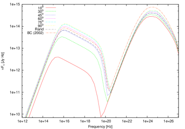
Figure 5: Synchrotron self-Compton spectra at a viewing angle of $0.014^{o}$ ($0.57^{o}$ in jet frame). The spectra shown results of different B-field configurations, including when it is randomly oriented in different cells. The plot shows $\theta_{B}$ values ($\phi_{B}=90^{o}$, unless randomly oriented). The red dot-dot-dashed curve shows the corresponding calculation based on the angle averaged emissivity and spherical geometry, using the code of Böttcher & Chiang (2002). See figure 2 for details on various angles.

Figure 6: Synchrotron self-Compton spectra at a various viewing angles (jet frame values). The B-field orientation: $\theta_{B}=45^{o}$, $\phi_{B}=90^{o}$. See figure 2 for details on various angles.

In order to study the effects of the B-field orientation on the synchrotron and synchrotron self-Compton spectra, we set up two scenarios. In the first set up the magnetic field is uni-directional in all the cells (27 in total) and in the second scenario the magnetic field is randomly oriented in each of the cells. These set-ups are likely to be the two extreme scenarios for a jet. Evidence points to the B-field being semi-ordered in AGN jets; for example, helical (Attridge et al., 1999; Lyutikov et al., 2005; Marscher et al., 2008). In all the presented cases, the electron distribution is a power-law and distributed uniformly over the angles $\theta$ and $\phi$.

Figure 5 shows synchrotron self-Compton spectra with different B-field configurations. Various simulation parameters can be found in table 1. The spectra are for a fixed viewing angle. Changing the B-field orientation has a significant impact on the observed spectrum. There is a large difference in flux values depending on the B-field orientation with respect to the observing direction. The minimum flux levels are observed at an orientation along the viewing angle while the maximum flux levels are observed when the B-field is perpendicular to the line of sight. The figure also demonstrates the fact that only the synchrotron spectrum component is heavily affected by the B-field orientation. The Compton scattered component of the spectrum is almost independent of the B-field orientation. The main reason for this is that the photon distribution anisotropies introduced by the B-field orientation are lost when scattering off an isotropic distribution of electrons. The small variations that remain are due to the $1-\beta\cos\psi$ factor present in Compton emissivity calculations. The line of sight and photon anisotropies therefore affect the extent to which the Compton spectrum is boosted. Additional anisotropies are introduced by the discretization of the photon and the electron angular distributions.

Figure 5 also shows a comparison with another SSC calculation (Böttcher & Chiang, 2002) which assumes a randomly oriented magnetic field. This simulation is set up with identical parameters to the ones outlined in table 1, except it uses a spherical volume instead of a cube; the total volumes are identical, therefore the sphere has a radius of $1.86\times 10^{14}$ cm. We can see that the synchrotron components are in good agreement. However, the Compton component in the Böttcher & Chiang (2002) calculation is much higher. The inverse Compton to synchrotron ratio $F_{IC}/F_{syn}$ differs by a factor $\sim$0.68 between the two calculations. This is most likely due to differing geometries. For a sphere, the average photon escape time is ${3R/4c}$, whereas in our cubic set up, due to the way radiation transport between cells is treated (see Section 2.1), a photon takes, on average, $2d_{cell}/c$ to escape the region ($d_{cell}$ is the width of an individual cell). Since the flux ratio $F_{SSC}/F_{syn}=u_{\rm syn}/u_{B}$ and the volume-averaged radiation energy density $u_{\rm syn}$ is proportional to the photon escape time scale, the longer photon escape time scale in the spherical geometry results in a larger SSC flux.

Figures 6 shows the effects of the viewing angle on the spectrum. It shows SEDs for a fixed azimuthal angle, but different viewing angles with a single B-field configuration. As before, there are normalization differences between the SEDs when comparing uniform and randomly oriented B-field, but the main factor in this case is the variation in the Doppler boosting due different viewing angles.

Parameter	fig 5 & 6
Cells	27
Cell size	$1\times 10^{14}$ cm
z	0.031
$\Gamma$	20.0
$u_{e}$	$9$ ergs cm-3
p	3.5
$\gamma_{min}$	$5\times 10^{3}$
$\gamma_{max}$	$5\times 10^{5}$
B	$0.9~{}\mathrm{G}$

Table 1: The simulation parameters for the results show in figures 5 and 6. Key to symbols: z = redshift, $\Gamma$ = Jet Lorentz factor, $u_{e}$ = electrons energy density, $p$ electrons distribution power law index, $\gamma_{min,max}$ = electrons distribution minimum and maximum energy, $B$ = B-field strength

3.1 Markarian 421

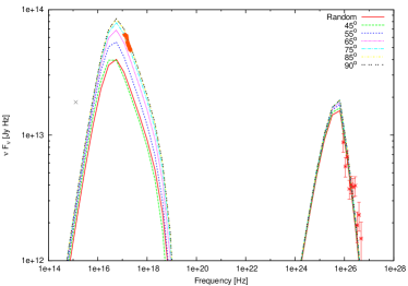
Figure 7: Synchrotron self-Compton fit for Markarian 421. The spectral fits are at various B-field orientations. The data are from XMM-Newton OM, XMM-Newton EPIC, and VERITAS. See table 2 for the fit parameters.

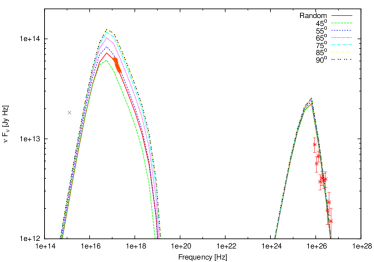
Figure 8: Synchrotron self-Compton fit for Markarian 421. The spectral fits are at various B-field orientations. The data are from XMM-Newton OM, XMM-Newton EPIC, and VERITAS. See table 2 for the fit parameters.

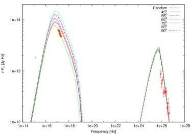
Figure 9: Synchrotron self-Compton fit for Markarian 421. The spectral fits are at various B-field orientations. The data are from XMM-Newton OM, XMM-Newton EPIC, and VERITAS. See table 2 for the fit parameters.

Markarian 421 was the first extragalactic source to be detected in TeV energies, hence making it an extensively studied source. We present spectral fits to XMM-Newton and VERITAS data presented in Acciari et al. (2009). We refer the reader to the above paper for the details on data reduction.

Figures 7, 8, and 9 show fits to Mrk 421 data using our code. Our aim in the present paper is to explore the impact of the B-field orientation on the fit parameters, especially the B-field estimates. In figure 7 we can see that the synchrotron component is best fit for a particular B-field orientation (see table 2 for fit parameters). The gamma-ray data, however, is fit well with all the orientations. This is due the fact that the self-Compton spectrum is not affected much by the B-field orientation (see the discussion in the previous section). There is a significant difference in the synchrotron peak when comparing various B-field orientations. The spectra in figure 7 show that at a good fit is achieved when the B-field is oriented at $85^{o}$ with a strength of $0.18$ G. However, the fit shown is not unique. We can see in figures 8 and 9 that for identical parameters, except the B-field strength, the best-fit B-field orientation is very different. In one case a pseudo-random B-field provides the best fit with $B=0.22$ G, while for $B=0.25$ G, a B-field orientation of $45^{o}$ provides the best fit. Therefore good fits can be achieved with different B-field strengths at different orientations. The main point here is the fact that it is possible to over- or underestimate the B-field strength when assuming it to be randomly oriented. In the cases presented here, the B-field strength ranges from 0.18 G to 0.25 G for very similar fits to the data, but with different magnetic-field orientations. Therefore it is possible to overestimate the magnetic field strength by at least $30\%$ if a particular B-field orientation, whether uniform or tangled, is assumed. If the B-field were pointed closely aligned with the line of sight, much higher B-field values will be necessary to obtain similar fits (see discussion in section 1.1). We also note that the bulk Lorentz factor used in the fits are lower than the values obtained by some authors for fitting Mrk 421 data (e.g. see Aleksic et al., 2011). The value of the bulk Lorentz factor values used in our fits is likely to be on the lower end of the limits imposed by pair opacity arguments (Celotti et al., 1998). However, the main point of this paper is not the determination of actual best-fit values for Mrk 421 (which would not be realistic due to our neglect of cooling effects anyway), but to demonstrate the orientation-dependent magnetic-field degeneracy in the course of blazar SED fitting.

Parameter	fig 7	fig 8	fig 9
Cells	27	27	27
Cell size	$3\times 10^{15}$ cm	$3\times 10^{15}$ cm	$3\times 10^{15}$ cm
z	0.031	0.031	0.031
$\Gamma$	10.0	10.0	10.0
$u_{e}$	$0.01$ ergs cm-3	$0.01$ ergs cm-3	$0.01$ ergs cm-3
p	4.1	4.1	4.1
$\gamma_{min}$	$3.7\times 10^{4}$	$3.7\times 10^{4}$	$3.7\times 10^{4}$
$\gamma_{max}$	$5\times 10^{5}$	$5\times 10^{5}$	$5\times 10^{5}$
B	$0.18~{}\mathrm{G}$	$0.22~{}\mathrm{G}$	$0.25~{}\mathrm{G}$

Table 2: Fit parameters for the Markarian 421 data shown in figures 7 and 8. Key to symbols: z = redshift, $\Gamma$ = Jet Lorentz factor, $u_{e}$ = electrons energy density, $p$ electrons distribution power law index, $\gamma_{min,max}$ = electrons distribution minimum and maximum energy, $B$ = B-field strength

4 Conclusions

In this paper we have presented first results from a new relativistic jet radiation transfer code that we are currently developing. Here we take the full angular dependence into account when modelling synchrotron and synchrotron self-Compton processes. We are able to model the B-field at arbitrary orientations and study its impact on the resulting spectra.

We have seen that the B-field orientation plays an important role on the normalization of the synchrotron spectrum. Using fits to Markarian 421 data, we have shown how the B-field orientation can mislead into over/under-estimating its strength. Any future work should therefore be mindful of the fact that the underlying assumption about the B-field orientation will play a considerable role in the errors associated with the magnetic field strength estimates.

References

- Acciari et al. (2009) Acciari, V. A., et al. 2009, ApJ, 703, 169
- Aleksic et al. (2011) Aleksic, J., et al. 2011, A&A
- Attridge et al. (1999) Attridge, J. M., Roberts, D. H., & Wardle, J. F. C. 1999, The Astrophysical Journal Letters, 518, L87
- Böttcher (2007) Böttcher, M. 2007, Astrophys. & Space Science, 309, 95
- Böttcher & Chiang (2002) Böttcher, M., & Chiang, J. 2002, The Astrophysical Journal, 581, 127
- Celotti et al. (1998) Celotti, A., Fabian, A. C., & Rees, M. J. 1998, Mon. Not. R. Astron. Soc., 293, 239
- Dermer & Menon (2009) Dermer, C. D., & Menon, G. 2009, High Energy Radiation from Black Holes: Gamma Rays, Cosmic Rays, and Neutrinos, ed. Dermer, C. D. & Menon, G.
- Dermer et al. (1992) Dermer, C. D., Schlickeiser, R., & Mastichiadis, A. 1992, Astronomy and Astrophysics, 256, L27
- Ghisellini & Madau (1996) Ghisellini, G., & Madau, P. 1996, Mon. Not. R. Astron. Soc., 280, 67
- Longair (1994) Longair, M. S. 1994, High energy astrophysics. Vol.2: Stars, the galaxy and the interstellar medium (Cambridge: Cambridge University Press, —c1994, 2nd ed.)
- Lyutikov et al. (2005) Lyutikov, M., Pariev, V. I., & Gabuzda, D. C. 2005, Mon. Not. R. Astron. Soc., 360, 869
- Mannheim & Biermann (1992) Mannheim, K., & Biermann, P. L. 1992, Astronomy and Astrophysics, 253, L21
- Maraschi et al. (1992) Maraschi, L., Ghisellini, G., & Celotti, A. 1992, The Astrophysical Journal Letters, 397, L5
- Marscher & Gear (1985) Marscher, A. P., & Gear, W. K. 1985, The Astrophysical Journal, 298, 114
- Marscher et al. (2008) Marscher, A. P., et al. 2008, Nature, 452, 966
- Mücke & Protheroe (2001) Mücke, A., & Protheroe, R. J. 2001, Astropart. Phys., 15, 121
- Mücke et al. (2003) Mücke, A., Protheroe, R. J., Engel, R., Rachen, J. P., & Stanev, T. 2003, Astropart. Phys., 18, 593
- Umstätter (1981) Umstätter, H, H. 1981, Efficient computation of synchrotron radiation spectrum, Tech. Rep. CERN-PS-SM-81-13, CERN, Geneva
- Wright (2006) Wright, E. L. 2006, The Publications of the Astronomical Society of the Pacific, 118, 1711