Predicting the number of giant arcs expected in the next generation wide-field surveys from space

Abstract

In this paper we estimate the number of gravitational arcs detectable in a wide-field survey such as that which will be operated by the Euclid space mission, assuming a $\Lambda$CDM cosmology. We use the publicly available code moka to obtain realistic deflection angle maps of mock gravitational lenses. The maps are processed by a ray-tracing code to estimate the strong lensing cross sections of each lens. Our procedure involves 1) the generation of a light-cone which is populated with lenses drawn from a theoretical mass-function; 2) the modeling of each single lens using a triaxial halo with a NFW (Navarro-Frenk-White) density profile and theoretical concentration-mass relation, including substructures, 3) the determination of the lensing cross section as a function of redshift for each lens in the light-cone, 4) the simulation of mock observations to characterize the redshift distribution of sources that will be detectable in the Euclid images. We focus on the so-called giant arcs, i.e. gravitational arcs characterized by large length-to-width ratios $(l/w\geq 5,7.5$ and 10). We quantify the arc detectability at different significances above the level of the background. Performing $128$ different realizations of a 15,000 sq. degree survey, we find that the number of arcs detectable at $1\sigma$ above the local background will be $8912_{-73}^{+79}$, $2914_{-25}^{+38}$, and $1275_{-15}^{+22}$ for $l/w\geq 5$, $7.5$ and $10$, respectively. The expected arc numbers decrease to $2409_{-28}^{+24}$, $790_{-12}^{+10}$, and $346_{-6}^{+6}$ for a detection limit at $3\sigma$ above the background level. From our analysis, we find that most of the lenses which contribute to the lensing optical depth are located at redshifts $0.4<z_{l}<0.7$ and that the $50\%$ of the arcs are images of sources at $z_{s}>3$. This is the first step towards the full characterization of the population of strong lenses that will be observed by Euclid. Given these results, we conclude that Euclid is a powerful instrument for strong lensing related science, which will be useful for several applications, ranging from arc and Einstein ring statistics to the measurement of the matter content in the cluster cores.

1 Introduction

It is unanimously recognized that galaxy clusters are objects of enormous cosmological importance. The reasons are manyfold. First, in the framework of the model of hierarchical structure formation, these are the latest structures to form, being the most massive. Second, they sample the exponential tail of the mass function, thus their abundance as a function of time is strongly sensitive to the values of cosmological parameters (Press & Schechter, 1974; Lacey & Cole, 1993; Sheth & Tormen, 2002). Third, compared to galaxies, their internal structure is less affected by baryons due to their small age, which implies that they are ideal laboratories to study the build up of the cosmic structure as predicted by the theory of Cold Dark Matter (CDM). Several clusters have been captured in the middle of a merging phase leading to the formation of a larger structure. The interplay between baryons and dark matter during such violent events highlights the fundamentally different behavior of the cluster mass components, providing wealth of information on what is the nature of dark matter. Alternatively, in those systems which appear to be relaxed, other predictions of the CDM theory can be tested, such as that the density profiles of dark-matter halos should converge to a (nearly) universal law, as originally found by Navarro et al. (1997).

An increasing number of observational campaigns are targeting galaxy clusters with the aim of using them as cosmological probes. They explore the whole wavelength range where clusters can be detected, from the X-ray (Böhringer et al., 2001; Murray et al., 2005), to the optical (Egami et al., 2007; Gal-Yam et al., 2005), to the radio (Raccanelli et al., 2012), to the millimeter (Swetz et al., 2011; Carlstrom et al., 2011; Planck Collaboration et al., 2011) wavelength ranges. These observations complement each other to reach a comprehensive view of how visible and invisible matter components are distributed. Several techniques have been developed to this goal. For example, in the optical domain, a direct method to investigate the distribution of matter is via the gravitational lensing effect. Due to their huge mass, galaxy clusters are the most powerful gravitational lenses observable in the sky. The light emitted by distant galaxies, which happens to travel through the space-time perturbed by a cluster gravitational potential, is deflected, causing a number of observable effects, like distortions, magnifications, and image multiplications. Since galaxy clusters extend over areas of many arc minutes squared, all lensing regimes can be observed around these systems. Galaxies located at large angular distances from the cluster center are weakly but coherently sheared tangentially to the cluster. Sources at smaller angular distances from the cluster center can be split into multiple images and/or appear as very elongated arcs. Both the weak and the strong lensing regimes can be inverted to derive information on the cluster mass distribution. In particular, their combination allows to derive precise measurements of the mass profiles from scales of few tens of kpc to the virial radius (see e.g. Meneghetti et al., 2010b; Giocoli et al., 2012b).

Among those which will investigate galaxy clusters via their lensing effects, the survey which will be operated by the Euclid mission (Laureijs et al., 2011) is likely to provide the highest quality data and the widest sky coverage. Euclid has been recently selected by ESA as medium-class space mission to be launched in 2019. It consists of a $1.2$m space telescope which will observe the sky both in the optical and in the near-infrared domains. In the optical, imaging will be taken to the nominal depth of 24.5 AB magnitudes in a wide $riz$ filter ($10\sigma$ extended sources). The telescope will be sensitive to photons at wavelengths between $0.55$ and $0.9\mu$m. For the same fields, Euclid will deliver imaging in the $Y,J,H$ NIR bands as well as slitless spectra covering the wavelength range $1.1-2.0\mu$m. The main survey which will be operated by Euclid is a 15,000 sq. degree wide survey of the sky at galactic latitudes $|b|>30$ deg. Euclid wants to use two primary probes to investigate the dark components of the Universe. These probes are weak-gravitational lensing by the large-scale structure of the Universe, Galaxy Clustering and the Baryonic-Acoustic-Oscillations. However, within the surveyed area, Euclid is expected to observe several tens of thousands of galaxy clusters. With the telescope design being developed under the driving requirement of allowing weak-lensing measurements of unprecedented quality, lensing will be the ideal method to investigate the matter content of these structures.

Not only Euclid will be a powerful instrument to investigate the weak-lensing regime, but it will also deliver high quality data suitable for the strong lensing analysis. Given the high resolution (0.1”/pixel) and sensitivity, Euclid will be able to detect and resolve with sufficient accuracy several strong lensing features arising from highly magnified distant galaxies near the cluster cores, and use them in combination with weak-lensing to extend the mapping of the cluster content to the central regions.

Additionally, strong lensing will be also used to constrain both cosmological parameters and the cluster properties following a more statistical approach. It has been shown by several authors that the number of strong lensing features on the whole sky is strongly dependent on 1) the geometrical properties of the universe; 2) the abundance of strong lenses as a function of redshift; and 3) several cluster properties, such as the average density profile, the masses, the three-dimensional shape, the concentration, the amount of substructures, the dynamical state, etc. Strong lensing statistics is therefore a potentially powerful tool to constrain cosmology and to trace the structure formation (Wambsganss et al., 1995, 1998). This argument holds in particular for very rare features like giant arcs, i.e. gravitational arcs characterized by large values of their length-to-width ratio, $(l/w)\geq(l/w)_{\rm min}$. The usage of giant arcs statistics for constraining the cosmological model was proposed by Bartelmann et al. (1998), who noted that the expected abundance of such events differs by orders-of-magnitude between cosmological models. Intriguingly, their simulations leaded to the conclusion that the number of arcs predicted in the currently favored $\Lambda$CDM cosmology is about one order-of-magnitude smaller than observed in samples of X-ray selected galaxy clusters (Le Fevre et al., 1994; Luppino et al., 1999). Further investigations on optically selected clusters found that the frequency of giant arcs is particularly high at redshifts $z\gtrsim 0.5$ (Zaritsky & Gonzalez, 2003; Gonzalez et al., 2003; Horesh et al., 2010).

The mismatch between arc statistics and other cosmological probes has been tagged as the arc statistics problem (Meneghetti et al., 2003). A number of studies have been conducted with the aim of explaining its origin (e.g. Dalal et al., 2004; Bartelmann et al., 2003b; Torri et al., 2004; Puchwein et al., 2005; Meneghetti et al., 2007; Wambsganss et al., 2008; Mead et al., 2010; Horesh et al., 2005, 2011; Li et al., 2005; Li et al., 2006; Wambsganss et al., 2004, 2005), but the controversy is not yet solved. Indeed, it was recently enforced by several other observations of strong lensing clusters, which seem to indicate that 1) some galaxy clusters have very extended Einstein rings (i.e. critical lines) whose abundances can hardly be reproduced by cluster models in the framework of a $\Lambda$CDM cosmology (Tasitsiomi et al., 2004; Broadhurst & Barkana, 2008b), and 2) several clusters, for which high-quality strong- and weak-lensing data became available, have concentrations that are far too high compared to the theoretical expectations (Broadhurst et al., 2008a; Zitrin et al., 2009). These evidences push in the same direction of the arc statistics problem, in the sense that they both suggest that observed galaxy clusters are strong lenses that are too effective compared to numerically simulated clusters. Current cluster surveys like CLASH (Cluster Lensing And Supernova survey with Hubble Postman et al. (2012)) are addressing these issues and will help to substantially understand the internal structure and the peculiarities of strong lensing clusters.

Existing gravitational arc surveys are based on cluster samples of limited size (few tens of galaxy clusters). Euclid will allow to dramatically increase the number of available strong lenses: on the basis of simple extrapolations, it is likely that thousands of arcs will be detected in the Euclid wide survey (Laureijs et al., 2011). In this paper, we aim at making robust estimates on the number of giant arcs which will be detectable in future Euclid observations. In particular, we wish to quantify the expected number of such arcs in a reference WMAP-7 normalized cosmological framework (Komatsu et al., 2011) with $\Omega_{0,m}=0.272$, $\Omega_{\Lambda}=0.728$, $h=0.704$ and $\sigma_{8}=0.809$. The goal is to provide hints on what kind of cluster strong-lensing related science will be possible with Euclid.

The paper is organized as follows: in Sect. 2 we introduce the relevant lensing quantities and we describe the methods used to compute the number of arcs.; in Sect 3, we discuss the results of the simulations, focussing in particular on the dependence of the expected number of arcs on the lens and source redshifts and finally, in Sect. 4, we draw our conclusions.

2 Analysis

2.1 Synthetic halos

Our theoretical expectations are based on the analysis of a set of synthetic halos generated with the public code MOKA Giocoli et al. (2012a). This code was recently developed by us with the aim of speeding up strong lensing calculations. It is well known that accurate estimates of the ability of clusters to produce strong lensing effects requires high level of details in cluster modeling (Meneghetti et al., 2000, 2003c; Torri et al., 2004; Meneghetti et al., 2007; Meneghetti et al., 2010a). So far, the required complexity of the lens models was ensured only by numerical simulations, i.e. by clusters obtained from N-body and hydrodynamic simulations (Meneghetti et al., 2003a; Puchwein et al., 2005). MOKA allows to create mock lenses using a fast semi-analytic approach, through which all the cluster properties that are relevant for strong lensing are incorporated in the lenses. This is achieved by using simulation-calibrated analytical relations to describe the shape and the content of clusters. A detailed description of the code and its implementation can be found in Giocoli et al. (2012a). Very briefly:

• clusters are assumed to possess a triaxial dark matter halo. The axial-ratios describing the elongation of these halos are drawn following the prescriptions of Jing & Suto (2002). To each halo, a random orientation is assigned;

• dark matter is distributed in the halos such that the averaged azimuthal density profile resembles the Navarro-Frenk-White (NFW) density profile (Navarro et al., 1997). The halo concentration and its dependence on mass and redshift is modeled using the $c-M$ relation of Zhao et al. (2009). A concentration scatter is assumed, which is also based on the analysis of numerically simulated dark matter halos. These typically show that concentrations at fixed mass are log-normally distributed with a rms $\sim 0.25$, almost independent of redshift;

• dark matter substructures are added to the lens models according to the substructure mass function found by Giocoli et al. (2010). Their spatial distribution is modeled following the cumulative density distribution by Gao et al. (2004). Each substructure is approximated with a truncated Singular-Isothermal-Sphere;

• a central Brightest-Cluster-Galaxy (BCG) is added at the center of the dark matter halos. The stellar content of the BCG is approximated by a Hernquist (1990) density profile. We take into account the influence of the presence of the BCG on the dark matter distribution near the halo center using the recipe by Blumenthal et al. (1986), which analytically describes the adiabatic contraction. The influence of baryons settled on the halo center on the surrounding dark matter distribution has been studied both using analytical calculations and numerical simulations, and during the last years the problem has also been addressed from an observational point of view (Schulz et al., 2010). However recently Newman et al. (2011), modeling the triaxiality of Abell 383, have ruled out baryonic physics which serve to steepen the central dark matter profile. Nowadays this phenomenology is still an open debate both from a theoretical – where the dark matter behavior seems to strongly depend on the gas physics and treatment of the simulations – and an observational point of view, and further investigations are out of the purposes of this paper. However we want to stress that in the light of what has been shown by Giocoli et al. (2012a) in comparing the strong lensing cross sections of triaxial haloes without and with BCG plus adiabatic contraction, we expect to find a difference of the order of $5-10\%$ between clusters with and without adiabatic contraction.

The lensing properties of halos generated with MOKA were discussed by Giocoli et al. (2012a). Since we want our modeled strong lensing halos to be as similar as possible to numerically simulated galaxy clusters, we include all features that significantly influence the strong lensing behavior in our computation. We stress that these features are related only to the dark matter halo structural and geometrical nature, and to the BCG: the unique significant baryonic element for strong lensing analysis. In Giocoli et al. (2012a) is tested that all characteristics listed above are essential for an optimal reproducing of simulated galaxy clusters strong lensing behavior. Finally, it is also very important to note that MOKA is very efficient and allows to quickly generate a lens model within a few seconds of CPU time on a powerful personal computer. Since we aim at simulating a (almost) full-sky survey of strong lensing clusters and at sampling a large number of lines of sight, which requires generating a large number of lenses, in this work we use MOKA to produce the mass distributions which are then analyzed by means of ray-tracing methods.

2.2 Ray-tracing simulations and cross sections

By using MOKA, we generate three-dimensional cluster models, which we project along arbitrary lines-of-sight. The usage of a semi-analytic formalism allows to quickly compute for each projected mass distribution its deflection angle field on the lens plane. This is used to distort the images of a large number of background sources in order to compute the lens cross sections for giant arcs. The methods employed to measure the cross sections are explained in details elsewhere (see e.g. Meneghetti et al., 2000). Here, we only summarized briefly the procedure.

We use the lens deflection angle maps to trace bundles of light rays from the observer position back to a source plane at redshift $z_{\rm s}=2$. This is populated with an adaptive grid of elliptical sources, whose spatial resolution increases toward the caustics of the lens. The caustics are lines on the source plane along which the lensing magnification diverges. Therefore, those sources which will be placed near the caustics will be characterized by large magnifications. The magnifications induced by lensing can either be tangential (near the tangential caustic) or radial (near the radial caustic). The adaptive source refinement artificially increases the number of highly magnified and distorted images. In the following analysis, a statistical weight, $w_{i}$, which is related to the spatial resolution of the source grid at the source position, is assigned to each source. If $a$ is the area of one pixel of the highest resolution source grid, then the area on the source plane of which the $i$-th source is representative is given by $A_{i}=aw_{i}$. By collecting the rays hitting each source on the source plane, we produce distorted images of these sources on the lens plane. The images are analyzed individually by measuring their lengths and widths using the method outlined in Meneghetti et al. (2000).

We define the lensing cross section for giant arcs, $\sigma_{l/w}$, as

$$\sigma_{l/w}=\sum A_{i}\;,$$ (1)

where the sum is extended to all sources that produce at least one image with $(l/w)\geq(l/w)_{\rm min}$.

2.3 Redshift evolution of the cross sections

The cross section is sensitive to several lens properties and it depends on the cosmological parameters and the redshifts of the lens and of the sources. If we pack all the relevant lens properties into the vector of parameters $\vec{p}$ and the cosmological parameters into the vector $\vec{c}$, then the expected number of arcs with $(l/w)\geq(l/w)_{\rm min}$ and surface brightness larger than $S$ that the lens can produce is given by

$$N_{l/w}(\vec{p},\vec{c},z_{l},S)=\int_{z_{l}}^{\infty}\sigma_{l/w}(\vec{p},\vec{c},z_{\rm l},z_{\rm s})n(z_{\rm s},S)\mbox{d}z_{\rm s}\;,$$ (2)

where $z_{\rm l}$ and $z_{\rm s}$ are the lens and the source redshifts, respectively, and $n(z_{\rm s},S)$ is the number density of sources with surface brightness larger than $S$ at redshift $z_{\rm s}$.

As explained above, we measure the lens cross sections for a fixed source redshift, $z_{\rm s}=2$. The previous formula shows that the cross sections need to be measured at all redshifts above $z_{\rm l}$ in order to calculate the number of arcs expected from a single lens. In principle, this would imply running ray-tracing simulations for many source planes, which is computationally very demanding, given the number of lenses we are using in this work. Following Meneghetti et al. (2010a), we prefer to determine a scaling function to describe the redshift evolution of the cross section. To construct this scaling function we proceed as follows.

Although $\sigma_{l/w}$ depends on a large number of lens properties, $\vec{p}$, we can identify the mass as the primary parameter characterizing the lens. Then, fixing the cosmological framework, we can write:

$$\sigma_{l/w}(M,z_{\rm l},z_{\rm s})\equiv\langle\sigma_{l/w}(\vec{p},\vec{c},z_{\rm l},z_{\rm s})\rangle_{\vec{\tilde{p}}}\;,$$ (3)

where the average is taken over the remaining lens properties, $\vec{\tilde{p}}$ (i.e. substructure content, concentration, triaxiality and orientation). We start by producing halos with MOKA spanning three orders of magnitude in mass, in the range $[10^{13}-10^{16}]$, distributed over the redshift interval $[0-1.5]$. Halos are subdivided in 100 logarithmically equi-spaced mass bins and 50 linearly equi-spaced redshift bins. In each ($M,z_{\rm l}$) cell, we generate $100$ halos with varying properties, $\vec{\tilde{p}}$, to be used for ray-tracing simulations as explained above. Therefore, the number of lenses we should process is $100\times 50\times 100=500,000$, which is huge and computationally very demanding. The numerical study performed by Meneghetti et al. (2010a) shows that there is a minimal mass $M_{\rm min}(z_{\rm l})$ at each redshift below which halos are not capable to produce giant arcs. To reduce the computational time, we use their results to avoid the computation of the cross section of halos with $M(z_{\rm l})<M_{\rm min}(z_{\rm l})$, for which we assume that $\sigma_{l/w}=0$. This allows us to the reduce the number of halos to be processed using ray-tracing to $\sim 340,000$. The minimal mass adopted in our study is shown as a function of redshift in Fig. 1.

Figure 1: Minimal mass for producing giant arcs as a function of redshift, as derived from the simulations by Meneghetti et al. (2010a).

We measure $\sigma_{l/w}(M,z_{\rm l},z_{\rm s}=2)$ by averaging the cross sections of all halos in the ($M,z_{\rm l}$) cell. This allows us to obtain $\sigma_{l/w}(M,z_{\rm l},z_{\rm s}=2)$ on a grid in the ($M,z{\rm l}$) plane. Then, we use subsamples of 32 halos randomly chosen in each ($M,z_{\rm l}$) cell to repeat the calculation of the cross sections for source planes at 32 different redshifts between $z_{\rm l}$ and $z_{\rm s,max}=6$. These source planes are defined such to take into account how rapidly the strong lensing efficiency is expected to to grow with redshift. In particular, for each lens redshift $z_{\rm l}$, we use the lensing distance function

$$D_{\rm lens}\equiv\frac{D_{\rm ls}D_{\rm l}}{D_{\rm{\bf s}}}\;,$$ (4)

where $D_{\rm l}$ ,$D_{\rm s}$ and $D_{\rm ls}$ are the angular diameter distances between the observer and the lens plane, between the observer and the source plane, and between the lens and the source planes, respectively. We normalize these functions such that $D_{\rm lens}(z_{\rm s}=6)=1$, and we determine the redshifts of the source planes by uniformly sampling the normalized lensing distance at intervals $\Delta D_{\rm lens}=1/32$. In Fig. 2 we show the normalized lensing distances as a function of the source redshift for several lens redshift. Our method to define the redshifts of the source planes ensures that many more source planes are placed in the redshift range where the lensing distance grows rapidly, while less planes are placed where the $D_{\rm lens}$ function becomes flat.

A critical aspect of the ray-tracing simulations and of the measurement of the cross sections may be given by the assumed size of the source galaxies, which is redshift dependent. Gao et al. (2009) studied how strongly the lensing cross sections depend on the source sizes. They found that this dependency is very weak. However, as it does not delay the computation time, we include in our simulations the redshift evolution of the galaxy sizes, which is modeled as follows. Gao et al. (2009) used COSMOS data (Scoville et al., 2007) to measure the redshift evolution of the galaxy effective diameter up to redshift 3 (see their Fig. 1). The median effective diameter measured by Gao et al. (2009) as a function of redshift is shown in Fig. 3. The curve has been extended to redshift 6 by assuming no evolution of the galaxy sizes above $z=3$. We use this function for setting the size of the sources as a function of redshift in our ray-tracing simulations.

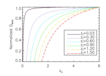
Figure 2: Normalized lensing distance as a function of $z_{s}$ for 5 different $z_{l}$ values, as shown in the label.

Having measured the cross sections for the different source planes, we can construct the scaling functions

$$f_{\sigma}(M,z_{\rm l},z_{\rm s})\equiv\dfrac{\sigma_{l/w}(M,z_{\rm l},z_{\rm s})}{\sigma_{l/w,0}(M,z_{\rm l},z_{\rm s}=2)}\;,$$ (5)

where $\sigma_{l/w}(M,z_{\rm l},z_{\rm s})$ is estimated by averaging over the 32 halos for each source plane. Some examples of the scaling functions for halos with mass $10^{15}h^{-1}M_{\odot}$ at several redshifts are shown in the Fig. 4. By construction all scaling functions intercept at $z_{\rm s}=2$, where $f_{\sigma}=1$. In Fig. 4, the thin lines that almost overlap the curves represent the scaling functions listed above computed without accounting for the source size dependence on redshift. As we can see, there is no remarkable difference among curves, hence we can state that source size dependence on redshift does not significantly affect the final number of arcs. Anyway, as already said, adding this feature does not change the computational time, so we decide to consider it in our implementation.

Figure 3: Apparent effective diameter as a function of redshift, as found by Gao et al. (2009).

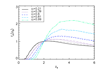
Figure 4: Median scaling functions derived from a sample of 32 lenses with $M\approx 10^{15}h^{-1}M_{\odot}$ for five $z_{l}$ values, as shown in the figure label. The thick (long-dashed) lines refer to functions computed without accounting for the source size dependence on redshift while thin lines are not.

Note that the scaling functions depend not only on the lens redshift, but also on the halo mass. This is clear in Fig 5, which shows the scaling functions measured at different redshifts and for halos of different mass. We see that, at any redshift, the scaling functions for low-mass lenses start to rise at larger $z_{s}$ compared to lenses with higher mass. They also tend to reach their maxima at significantly higher redshift. This is due to the fact that small lenses are efficient at producing giant arcs only when the sources are distant. Therefore, it is of fundamental importance to evaluate the scaling functions in different mass and redshift bins, as we do here.

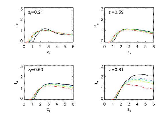
Figure 5: Scaling functions at four different lens redshifts. Starting from the upper left panel and continuing to the bottom right, the results refer to lenses at $z_{l}=0.21,0.39,0.6$ and $0.81$, respectively. In each plot we show the curves corresponding to five different masses, namely $2\times 10^{14}h^{-1}M_{\odot}$ (black solid line), $4.5\times 10^{14}h^{-1}M_{\odot}$ (blue dotted line), $7.5\times 10^{14}h^{-1}M_{\odot}$ (cyan dashed line), $10^{15}h^{-1}M_{\odot}$ (green dot-dashed line) and $3.2\times 10^{15}\,h^{-1}M_{\odot}$ (red double dot-dashed line).

By using the scaling functions, we can re-write Eq. 2 as

$$N_{l/w}(\vec{p},\vec{c},z_{l},S) = \sigma_{l/w}(\vec{p},\vec{c},z_{\rm l},z_{\rm s}=2)\times$$ (7)

$$\times\int_{z_{l}}^{\infty}f_{\sigma}(M,z_{\rm l},z_{\rm s})n(z_{\rm s},S)\mbox{d}z_{\rm s}\;,$$

which allows us to estimate the number of arcs produced by any lens for a given number density of sources just by measuring its cross section at $z_{\rm l}=2$.

2.4 Source number density

The last ingredient needed in Eq. 7 to be able to compute the number of giant arcs expected from a single lens is the number density of sources as a function of redshift and limiting surface brightness, $n(z_{\rm s},S)$.

For deriving the source redshift distribution function, we make use of simulated observations with the SkyLens software (Meneghetti et al., 2008; Meneghetti et al., 2010b; Bellagamba et al., 2012; Rasia et al., 2012). This code uses a set of real galaxies decomposed into shapelets (Refregier, 2003) to model the source morphologies on a synthetic sky. In particular, we use here 10,000 galaxies in the B, V,i,z bands from the Hubble-Ultra-Deep-Field (HUDF) archive (Beckwith et al., 2006). Most galaxies have spectral classifications and photometric redshifts available (Coe et al., 2006), which are used to generate a population of sources whose luminosity and redshift distributions resemble those of the HUDF. SkyLens allows us to mimic observations with a variety of telescopes, both from space and from the ground. For this work, we simulate wide-field observations with the optical camera which will be onboard the Euclid satellite. For setting up these simulations, we stick to the Euclid description (throughput, PSF, telescope size, CCD characteristics, etc.) contained in the Euclid Red-Book (Laureijs et al., 2011). More details on Euclid simulations carried out with the SkyLens software can be found in Bellagamba et al. (2012).

We simulate $400"\times 400"$ fields to the depth which will be reached by Euclid ($m_{riz}\sim 24.5$), and we derive the number density and the redshift distribution of all sources detected in the simulated images. To analyze the images, we use the software SExtractor (Bertin & Arnouts, 1996), which we use also to estimate the background rms. We derive source catalogs imposing different detection thresholds, i.e $1$ and $3$ times the background rms.

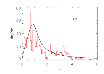
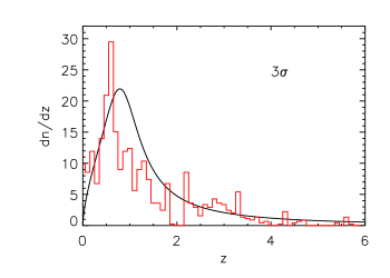
Figure 6: Source density distribution as a function of redshift for galaxies detected at 1$\sigma$ and 3$\sigma$ above the mean background level. The red histograms show the distributions derived from the analysis of the Euclid simulated observations. The solid lines show the best fit to the distributions using the functional proposed by Fu et al. (2008). Numbers in the $y$ axis are in unit of arcmin^-2.

The redshift distributions obtained for these two detection limits are shown by the histograms in Fig. 6, where we plot the number density of detected sources as a function of their redshift. We fit these distributions with the functional proposed by Fu et al. (2008), which has the form

$$n(z)=A\dfrac{z^{a}+z^{ab}}{z^{b}+c}\;,$$ (8)

with

$$A=\left(\int_{0}^{+\infty}\dfrac{z^{a}+z^{ab}}{z^{b}+c}\mbox{d}z\right)^{-1}$$

and $a,b,c$ free parameters. We find that the observed distributions are fitted by the functional with bets-fit parameters $(a,b,c)=(0.764,5.998,0.751)$ and $(a,b,c)=(0.662,5.502,0.633)$ for sources $1\sigma$ and $3\sigma$ above the mean sky level, respectively. These best fits are shown by the solid lines in Fig. 6 from the same figures.

2.5 Construction of the light-cones

The procedure outlined above describes how we can calculate the number of arcs with a given $l/w$ ratio produced by a single lens. By investigating all lenses on our $(M,z_{\rm l})$ grid, we end up with a list of $\sim 340,000$ cross sections for sources at redshift $z_{\rm s}=2$, which we can transform into cross sections for other source redshifts using the previously defined scaling functions. In particular, for each cell of the grid, we have $100$ cross sections of halos with similar mass but different structural properties.

In this section, we explain how we estimate the number of arcs expected in a given area of the sky. To achieve this goal, we obviously need to consider all lenses within the light-cone with vertex on the observer, which subtends the surveyed area. More specifically, aiming at simulating the wide survey which will be operated by Euclid, we construct light-cones subtending an area of 15,000 squared degree. The depth of the light-cones should be such to contain all lenses capable to produce giant arcs. According to the simulations by Meneghetti et al. (2010a), we expect no lenses producing giant arcs from sources at $z_{\rm s}=2$ above $z_{\rm l}\sim 1.3$. To be more conservative, given that our simulations use source planes until redshift $z_{\rm s}=6$, we extend the light-cones up to $z_{\rm l}=1.5$. It is worth mentioning, however, that a giant arc has been recently discovered behind the galaxy cluster IDCS J1426.5+3508 at $z=1.75$ using deep HST/ACS+WFC3 observations (Gonzalez et al., 2012a). On the basis of the arc color, the arc redshift has been constrained to be at $z<6$, most likely $z\sim 4$. The integrated magnitude in the F814W ACS filter is $24.29\pm 0.31$, thus close to the detection limit of Euclid. As we will show later, in our simulations no giant arcs are produced by lenses at $z_{\rm l}>1.3$. Thus, our results confirm the peculiarity of this arc detection, which may have interesting cosmological implications (Gonzalez et al., 2012a).

Once defined the size of the light-cones, we populate them with lenses with different mass and redshift. To do so, we divide the cone into $50$ redshift slices, equi-spaced in redshift with $\Delta z=0.03$. This is the same redshift spacing used to construct the grid $(M,z_{\rm l})$ over which the cross sections were evaluated. Thus, we define 50 lens planes, with the first plane at $z=0.03$ and the last plane placed at redshift $1.5$.

We calculate the number of the lenses with a given mass to be placed on each lens plane by using the Sheth & Tormen mass function (Sheth & Tormen, 1999). Masses are drawn again in the interval $[10^{13},10^{16}]\,h^{-1}M_{\odot}$. To consider effects of cosmic variance, we produce 128 realizations of the light-cone. The average number of halos generated in each redshift slice is shown by the solid line in Fig. 7, where the error-bars quantify the scatter between the different light-cone realizations.

Figure 7: Median number of halos as a function of redshift in the 128 realizations of the light cone corresponding to the Euclid wide survey. The error-bars indicate the minimum and maximum number of halos in each redshift bin, again from the 128 light-cone realizations.

To calculate the number of giant arcs expected to be detectable in the surveyed area, for each halo of mass $M$ and redshift $z_{\rm l}$, we randomly select one of the $100$ cross sections in the corresponding $(M,z_{\rm l})$ cell. Then, we assign to the halo the scaling function previously measured for halos with its mass and redshift. We use Eq. 7 to compute the number of arcs expected from each lens. The total number of arcs expected in the survey is then calculated as

$$N_{l/w}^{tot}=\sum_{i=1}^{N_{lens}}N_{l/w,i}\;,$$ (9)

where $N_{lens}$ is the total number of arcs in the light-cone and $N_{l/w,i}$ is the number of arcs produced by the $i$-th lens.

		$N_{med}$	I quartile	III quartile	$N_{min}$	$N_{max}$
$l/w\geq 5$	$1\sigma$	8912	8839	8991	8623	9308
	$3\sigma$	2409	2381	2433	2294	2482
$l/w\geq 7.5$	$1\sigma$	2914	2889	2952	2810	3100
	$3\sigma$	790	779	800	746	819
$l/w\geq 10$	$1\sigma$	1275	1260	1297	1216	1387
	$3\sigma$	346	340	352	323	362

Table 1: $N_{med}$ is the median number of arcs with $l/w\geq 5$, $7.5$, and $10$, computed from the results of 128 different $15,000$ deg² mock light-cone realizations, from sources $1\sigma$ and $3\sigma$ upon the mean sky level. In fourth and fifth columns are the 25% and 75% percentiles, while in sixth and seventh columns are the minimum and maximum values.

3 Results

In this section, we show the results of our analysis, discussing in particular the expected number of arcs in the Euclid wide survey and the number of arcs as a function of the lens and source redshifts.

3.1 The total number of arcs

The total number of arcs expected in the Euclid wide survey on the basis of our simulations is given in Tab. 1 for different minimal length-to-width ratios ($l/w_{\rm min}=5,7.5,10$) and for two detection thresholds, namely $1$ and $3$ times the background rms These values represent the threshold above the background for which a group of connected pixels are identified by SExtractor (Bertin & Arnouts, 1996). We report the median number of arcs derived from the 128 realizations of the light-cones ($N_{med}$), as well as the quartiles of the distributions. To allow for better quantification of the cosmic variance, we also report the minima and the maxima of the distributions.

If we consider the detections above the background rms, the median numbers of arcs with $l/w\geq 5$, $7.5$ and $10$ are $8912_{-73}^{+79}$, $2914_{-25}^{+38}$ and $1275_{-15}^{+22}$ respectively. If we consider the detections at higher significance ($3$ times the background rms) the respective numbers are $2409_{-28}^{+24}$, $790_{-12}^{+10}$ and $346\pm 6$. The quoted errors correspond to the inter-quartile ranges of the distributions. We notice that those values are dependent somehow on the source redshift distribution adopted, which is consistent with the simulations performed with the Euclid telescope equipment. A source redshift distribution with a pick shifted $10\%$ below or above our fiducial one produces a total number of arcs which is $20\%$ smaller or larger.

We would like to stress that these arcs will be potentially detectable in the future Euclid wide survey. At this stage, we are not considering several practical difficulties which may complicate the recognition of gravitational arcs in real observations. For example, arcs can be easily confused with edge-on spiral galaxies or with other elongated structures on the CCDs. Additionally, arcs form in dense regions of cluster galaxies. Since these are typically very bright and extended, arcs are frequently hidden behind them. Aiming at analyzing huge datasets such as the data that will be delivered by Euclid, it will be particularly important to develop softwares for the automatic detection of gravitational arcs. Few such tools exist already (Alard, 2006; Seidel & Bartelmann, 2007; Cabanac et al., 2007; More et al., 2012) and have been tested extensively. In a work in progress, we are currently addressing the task of quantifying the degree of contamination and completeness of the arc catalogs delivered from these arc finders through the analysis of simulated images.

Nevertheless, these results indicate that Euclid will be able to detect an unprecedented number of strong lensing features such as giant arcs and arclets. These will represent a treasury for any future study focusing not only on arc statistics but also aiming at using these features to construct and calibrate lens models and to map the mass distribution in galaxy clusters.

3.2 Arc production as a function of the lens redshift

It is interesting to study the redshift distribution of the lenses producing giant arcs. This is important to assess which lenses will be better constrained by strong lensing data. Moreover, given its sensitivity to the dynamical evolution of clusters, it is important to understand up to which redshift gravitational arcs can be used to trace cluster evolution.

In Fig. 8 we show the number of arcs produced by lenses at different redshifts. We use solid red, dashed orange and long-dashed green lines to display the results for arcs with $l/w\geq 5$, 7.5, and 10, respectively. Shown are the medians of the 128 realizations of the Euclid survey (thick lines) and the corresponding ranges among minimum and maximum values (thin lines). The left and the right panels refer to detections at the levels of $1$ and $3$ times the background rms

We note that, independently of the minimal $l/w$ ratio, the number of arcs reaches its maximum at redshift $\sim 0.6$. It drops quickly to zero at redshifts $z\lesssim 0.2$ and $z\gtrsim 1.2$. Such behavior results from a combination of different reasons. First, at low redshift, the cosmic volume contained in the light-cone is small, thus a relatively small number of lenses are present at these redshifts. This is clear from Fig. 7, which shows that the number of halos drops by almost two orders-of-magnitude between $z=0.4$ and $z=0.2$ and by an additional order-of-magnitude between $z=0.2$ and $z=0.1$. Second, the lensing cross section of individual halos is small both at low- and at high-redshift, i.e. when the lens is too close to the observer or to the bulk of sources. To illustrate this, we show in Fig. 9 the lensing cross section for arcs with $l/w\geq 7.5$ (solid lines) and $l/w\geq 10$ (dashed lines) as a function of redshift for a halo with mass $7\times 10^{14}\;h^{-1}\;M_{\odot}$. Given the redshift distribution of the sources expected in the Euclid observations, the median source redshift in the case of arcs detectable at the level of $1$ and $3$ times the background rms are $z_{s}=z_{s,1\sigma}^{med}=1.24$ and $z_{s}=z_{s,3\sigma}^{med}=1.03$, respectively. In the upper and bottom panels of Fig. 9, we use these source redshifts to calculate the cross sections. This explains why the curve in the upper panel reaches its maximum at a slightly larger redshift than the curve in the bottom panel. Third, as the redshift grows, increasingly less massive halos are expected, which implies that the number of gravitational arcs produced by these lenses is substantially lower. Fourth, although high-redshift sources can be more efficiently distorted, their surface brightness is dimmed, and their images are more difficult to detect.

As we can see from Fig. 9, the lensing cross sections of each individual halo exhibit several local maxima at different lens redshifts. We remind that MOKA produces mock lenses which include substructures whose mass and positions are drawn from recipes calibrated on numerical simulations. In particular, halos may be produced with mass configurations resembling a merging phase. In fact, the bumps in Fig. 9 correspond to such events, which are known to boost the lensing cross section and the production of arcs, (Torri et al., 2004) significantly. The same events are responsible for the irregular behavior of the curves in Fig. 8.

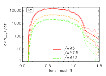
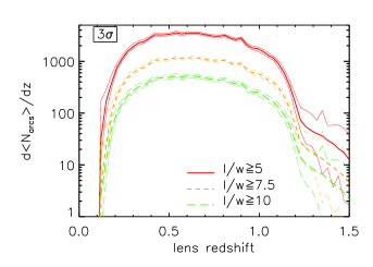
Figure 8: Number of arcs as a function of the lens redshift. The thick (thin) lines are the median (quartiles) among the 128 light-cone realizations and they refer to arcs with $l/w\geq 5$ (solid red), $7.5$ (dashed orange), and $10$ (long-dashed green), respectively. The left and the right panels refer to detections at the level of $1$ and $3$ times the background rms.

Figure 9: Lensing cross section as a function of the lens redshift for a halo with mass $7\times 10^{14}h^{-1}M_{\odot}$. The upper and the bottom panels refer to detections at the level of $1$ and $3$ times the background rms, respectively. The solid and the dashed lines indicate the cross sections for arc with $l/w\geq 7.5$ and with $l/w\geq 10$, respectively (cross sections for arcs with $l/w\geq 5$ have a similar behavior).

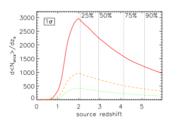
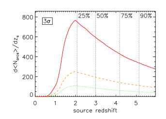
Figure 10: Number of arcs as a function of $z_{s}$. The left and the right panels refer to detections at the level of $1$ and $3$ times the background rms Results are shown for arcs with $l/w\geq 5$ (solid line), $7.5$ (dashed line), and $10$ (dotted line). The fractional numbers of arcs originated from sources at $z\leq z_{\rm s}$ are given by the vertical dotted lines: they are independent of the value of $l/w$.

3.3 Arc production as function of the source redshift

Now we discuss how the number of arcs expected from a Euclid-like wide survey varies as a function of the source redshift. This is useful to understand what will be the the typical redshift range of the sources strongly lensed by galaxy clusters, which provides interesting information on how accurately the lens mass profiles may be constrained.

Our results are summarized in Fig. 10, where we show the number of arcs produced by all lenses in the light-cone as a function of the source redshift. The solid, dashed, and dotted lines refer to arcs with $l/w\geq 5$, $7.5$, and $10$, respectively. As usual, we show the results for detections at the levels of $1$ and $3$ times the background rms (left and right panels). The results shown here are the medians over the 128 light-cone realizations. The vertical dotted lines indicate the cumulative fractional number of arcs originated by sources at redshifts $\leq z_{\rm s}$. All curves, are similar independently of the value $l/w$, have a maximum at $z_{\rm s}\sim 2$, indicating that the maximal efficiency for producing gravitational arcs is reached at this redshift. The number of arcs decreases quickly at lower redshifts. Only $\sim 25\%$ of the arcs is originated by sources at redshift $z_{\rm s}\lesssim 2$. On the contrary the vast majority of arcs are originated by sources at higher redshift: $\sim 50\%$ of them are originated by sources at $z_{\rm s}\gtrsim 3$. The figure shows that the arc number is expected to decline gently as a function of the source redshift, with $25\%$ and $10\%$ of them corresponding to sources at redshifts $\gtrsim 4.2$ and $\gtrsim 5.2$, respectively.

Therefore, our results reveal that Euclid, due to its high efficiency, will be an useful gravitational telescope and it will improve the study of distant galaxies (Zitrin et al., 2012).

4 Conclusions

In this work we outlined a method to calculate the number of giant arcs expected in a wide survey. We particularized our calculation to the case of the 15,000 sq. degrees survey which will be operated by the Euclid space mission starting in 2019. Our method is based on the publicly available code MOKA (Giocoli et al., 2012a), which allows to create realistic mock galaxy cluster deflection angle maps, including all features important for strong gravitational lensing features in a very short computational time. In particular it includes triaxiality, substructures, asymmetries, a CD galaxy, and adiabatic contraction due to baryons in cluster center. We recall that, since it uses recipes directly calibrated on N-body simulations, MOKA produces models that are fully consistent with numerical simulations (see e.g. Giocoli et al., 2012a).

For our analysis, we created a catalog of $\sim$ 340,000 mock galaxy clusters, spanning three orders of magnitude in mass and distributed over the redshift interval $0<z<1.5$, assuming a reference WMAP-7 normalized cosmology. Using ray-tracing techniques, we measured the strong lensing cross section for the production of giant arcs of each lens. We also estimated the evolution of the lensing cross sections as a function of the source redshift. We used the resulting catalog of lensing cross sections to generate 128 realizations of the $15,000$ sq. degrees survey, distributing mock lenses in light-cones spanning the redshift range $[0,1.5]$. We used the SkyLens code (Meneghetti et al., 2008) to produce realistic simulated observations by Euclid, which we used to determine the redshift distribution of the galaxies which are likely to be lensed by foreground clusters.

With so many realizations of the Euclid survey, we estimated the number of arcs, and its statistical uncertainty, which will be detectable in future Euclid observations at different detection limits. We discussed what is the typical redshift of lenses producing arcs as well as what is the redshift of sources that are lensed so as to produce arcs detectable by Euclid. Our results can be summarized as follows:

• Among the different realizations of the Euclid survey, the median numbers of arcs detectable at the level of $1\sigma$ above background level are $8912_{-73}^{+79}$, $2914_{-25}^{+38}$, and $1275_{-15}^{+22}$ for arcs with $l/w\geq 5$, $7.5$ and $10$, respectively; such numbers decrease to $2409_{-28}^{+24}$, $790_{-12}^{+10}$ and $346\pm 6$ for arcs detectable at the level of three times the local background rms The quoted errors reflect the first and the third quartiles of the arc number distribution.

• Most of the arcs are produced by lenses at redshifts in the range $[0.4,0.7]$. This is due to the large abundance of efficient lenses in this redshift range.

• We found that $50\%$ of the total number of arcs will be produced by galaxies at redshifts $z\gtrsim 3$. Additionally, $25\%$ and $10\%$ of the arcs will be produced by sources at $z>4.15$ and at $z>5.1$, respectively. Thus, lensed sources in the future Euclid observations will be detected up to very high redshift. Their redshift distribution will peak at $z\approx 2$, almost independent of the length-to-width ratio.

Given these results, we conclude that Euclid is a powerful instrument for strong lensing related science, which will be useful for several applications, ranging from arc and Einstein ring statistics to the measurement of the matter content in the cluster cores.

Several works in the literature tried to estimate how the expected number of arcs reacts to changing the values of cosmological parameters. For example, Bartelmann et al. (2003b) find that in models with dynamical dark energy we should expect of order of $20-25\%$ larger optical depths for strong lensing than in a $\Lambda$CDM cosmology. D’Aloisio & Natarajan (2011) show that variations of the same order of the expected number of arcs are expected in models with non-Gaussian initial conditions ($-5\%$ to $+45\%$ for f_NL varying between -10 and +74. Fedeli et al. (2008) find that the number of arcs changes by one order of magnitude if the power-spectrum normalization $\sigma_{8}$ is changed from 0.7 to 0.9. Our results indicate that, if we consider the statistical errors on the number of giant arcs alone, Euclid will be potentially able to discriminate between different models of dark energy, initial conditions, and cosmological parameters. With the procedure we have constructed in this work, we can easily compare different cosmological frameworks in a reasonable time and test whether future instruments such as Euclid will be able to use arc statistics as an additional cosmological probe.

AKNOWLEDGEMENTS

We thank Thomas Kitching and Henk Hoekstra for useful comments. We are grateful also to Matthias Bartelmann for interesting discussions. Many thanks also the the anonymous referee for helpful comments and suggestions. We acknowledge financial contributions from contracts I/009/10/0, EUCLID-IC phase A/B1, PRIN-INAF 2009, ASI-INAF I/023/05/0, ASI-INAF I/088/06/0, ASI I/016/07/0 COFIS, ASI Euclid-DUNE I/064/08/0, ASI-Uni Bologna-Astronomy Department Euclid-NIS I/039/10/0 and PRIN MIUR “dark energy and cosmology with large galaxy surveys”. CG’s research has been partially supported by the project GLENCO, funded under the Seventh Framework Programme, Ideas, Grant Agreement n. 259349. The simulations of this project have been run during the Class C Project-HP10CGR27W (MOKAlen1).

References

- Alard (2006) Alard C., 2006, ArXiv Astrophysics e-prints
- Bartelmann et al. (1998) Bartelmann M., Huss A., Colberg J. M., Jenkins A., Pearce F. R., 1998, A&A, 330, 1
- Bartelmann et al. (2003b) Bartelmann M., Meneghetti M., Perrotta F., Baccigalupi C., Moscardini L., 2003b, A&A, 409, 449
- Beckwith et al. (2006) Beckwith S. V. W., Stiavelli M., Koekemoer A. M., Caldwell J. A. R., Ferguson H. C., Hook R., Lucas R. A., Bergeron L. E., Corbin M., Jogee S., et al. 2006, AJ, 132, 1729
- Bellagamba et al. (2012) Bellagamba F., Meneghetti M., Moscardini L., Bolzonella M., 2012, MNRAS, 422, 553
- Bertin & Arnouts (1996) Bertin E., Arnouts S., 1996, A&AS, 117, 393
- Blumenthal et al. (1986) Blumenthal G. R., Faber S. M., Flores R., Primack J. R., 1986, ApJ, 301, 27
- Böhringer et al. (2001) Böhringer H., Schuecker P., Guzzo L., Collins C. A., Voges W., Schindler S., Neumann D. M., Cruddace R. G., De Grandi S., Chincarini G., Edge A. C., MacGillivray H. T., Shaver P., 2001, A&A, 369, 826
- Broadhurst et al. (2008a) Broadhurst T., Umetsu K., Medezinski E., Oguri M., Rephaeli Y., 2008a, ApJ, 685, L9
- Broadhurst & Barkana (2008b) Broadhurst T. J., Barkana R., 2008b, MNRAS, 390, 1647
- Cabanac et al. (2007) Cabanac R. A., Alard C., Dantel-Fort M., Fort B., Gavazzi R., Gomez P., Kneib J. P., Le Fèvre O., Mellier Y., Pello R., Soucail G., Sygnet J. F., Valls-Gabaud D., 2007, A&A, 461, 813
- Carlstrom et al. (2011) Carlstrom J. E., Ade P. A. R., Aird K. A., Benson B. A., Bleem L. E., Busetti S., Chang C. L., Chauvin E., Cho H.-M., Crawford T. M., et al. 2011, PASP, 123, 568
- Coe et al. (2006) Coe D., Benítez N., Sánchez S. F., Jee M., Bouwens R., Ford H., 2006, AJ, 132, 926
- Dalal et al. (2004) Dalal N., Holder G., Hennawi J. F., 2004, ApJ, 609, 50
- D’Aloisio & Natarajan (2011) D’Aloisio A., Natarajan P., 2011, MNRAS, 415, 1913
- Egami et al. (2007) Egami E., Marshall P., Mazzotta P., Evrard A., Carlstrom J., Smith G. P., Kneib J.-P., Finoguenov A., Futamase T., Taylor J., 2007, NOAO Proposal, p. 451
- Fedeli et al. (2008) Fedeli C., Bartelmann M., Meneghetti M., Moscardini L., 2008, A&A, 486, 35
- Fu et al. (2008) Fu L., Semboloni E., Hoekstra H., Kilbinger M., van Waerbeke L., Tereno I., Mellier Y., Heymans C., Coupon J., Benabed K., Benjamin J., Bertin E., Doré O., Hudson M. J., Ilbert O., Maoli et al. 2008, A&A, 479, 9
- Gal-Yam et al. (2005) Gal-Yam A., Cenko S. B., Fox D. W., Leonard D. C., Moon D.-S., Sand D. J., Soderberg A. M., 2005, in Turatto M., Benetti S., Zampieri L., Shea W., eds, 1604-2004: Supernovae as Cosmological Lighthouses Vol. 342 of Astronomical Society of the Pacific Conference Series, The Caltech Core-Collapse Project (CCCP). p. 305
- Gao et al. (2009) Gao G. J., Jing Y. P., Mao S., Li G. L., Kong X., 2009, ApJ, 707, 472
- Gao et al. (2004) Gao L., White S. D. M., Jenkins A., Stoehr F., Springel V., 2004, MNRAS, 355, 819
- Giocoli et al. (2012a) Giocoli C., Meneghetti M., Bartelmann M., Moscardini L., Boldrin M., 2012a, MNRAS, 421, 3343
- Giocoli et al. (2012b) Giocoli C., Meneghetti M., Ettori S., Moscardini L., 2012b, MNRAS, 426, 1558
- Giocoli et al. (2010) Giocoli C., Tormen G., Sheth R. K., van den Bosch F. C., 2010, MNRAS, 404, 502
- Gonzalez et al. (2012a) Gonzalez A. H., Stanford S. A., Brodwin M., Fedeli C., Dey A., Eisenhardt P. R. M., Mancone C., Stern D., Zeimann G., 2012, ArXiv e-prints
- Gonzalez et al. (2003) Gonzalez A. H., Zabludoff A. I., Zaritsky D., 2003, Ap&SS, 285, 67
- Hernquist (1990) Hernquist L., 1990, ApJ, 356, 359
- Horesh et al. (2005) Horesh A., Ofek E. O., Maoz D., et al. 2005, ApJ, 633, 768
- Horesh et al. (2010) Horesh A., Maoz D., Ebeling H., Seidel G., Bartelmann M. 2010, MNRAS, 406, 1318
- Horesh et al. (2011) Horesh A., Maoz D., Hilbert S., Bartelmann M.2011, MNRAS, 418, 54
- Jing & Suto (2002) Jing Y. P., Suto Y., 2002, ApJ, 574, 538
- Komatsu et al. (2011) Komatsu E., Smith K. M., Dunkley J., Bennett C. L., Gold B., Hinshaw G., Jarosik N., Larson D., et al. 2011, ApJS, 192, 18
- Lacey & Cole (1993) Lacey C., Cole S., 1993, MNRAS, 262, 627
- Laureijs et al. (2011) Laureijs R., Amiaux J., Arduini S., Auguères J. ., Brinchmann J., Cole R., Cropper M., Dabin C., Duvet L., et al. 2011, ArXiv e-prints
- Le Fevre et al. (1994) Le Fevre O., Hammer F., Angonin M. C., Gioia I. M., Luppino G. A., 1994, ApJ, 422, L5
- Li et al. (2005) Li G.-L., Mao S., Jing Y. P., et al. 2005, ApJ, 635, 795
- Li et al. (2006) Li G. L., Mao S., Jing Y. P., et al. 2006, MNRAS, 372, L73
- Luppino et al. (1999) Luppino G. A., Gioia I. M., Hammer F., Le Fèvre O., Annis J. A., 1999, A&AS, 136, 117
- Mead et al. (2010) Mead J. M. G., King L. J., Sijacki D., Leonard A., Puchwein E., McCarthy I. G., 2010, MNRAS, 406, 434
- Meneghetti et al. (2007) Meneghetti M., Argazzi R., Pace F., Moscardini L., Dolag K., Bartelmann M., Li G., Oguri M., 2007, A&A, 461, 25
- Meneghetti et al. (2003a) Meneghetti M., Bartelmann M., Moscardini L., 2003a, MNRAS, 340, 105
- Meneghetti et al. (2003c) Meneghetti M., Bartelmann M., Moscardini L., 2003c, MNRAS, 346, 67
- Meneghetti et al. (2003) Meneghetti M., Bartelmann M., Moscardini L., Rasia E., Tormen G., Torri E., 2003, ArXiv Astrophysics e-prints
- Meneghetti et al. (2000) Meneghetti M., Bolzonella M., Bartelmann M., Moscardini L., Tormen G., 2000, MNRAS, 314, 338
- Meneghetti et al. (2010a) Meneghetti M., Fedeli C., Pace F., Gottlöber S., Yepes G., 2010a, A&A, 519, A90+
- Meneghetti et al. (2008) Meneghetti M., Melchior P., Grazian A., De Lucia G., Dolag K., Bartelmann M., Heymans C., Moscardini L., Radovich M., 2008, A&A, 482, 403
- Meneghetti et al. (2010b) Meneghetti M., Rasia E., Merten J., Bellagamba F., Ettori S., Mazzotta P., Dolag K., Marri S., 2010b, A&A, 514, A93+
- More et al. (2012) More A., Cabanac R., More S., Alard C., Limousin M., Kneib J.-P., Gavazzi R., Motta V., 2012, ApJ, 749, 38
- Murray et al. (2005) Murray S. S., Kenter A., Forman W. R., Jones C., Green P. J., Kochanek C. S., Vikhlinin A., Fabricant D., Fazio G., Brand K., Brown M. J. I., Dey A., Jannuzi B. T., Najita J., McNamara B., Shields J., Rieke M., 2005, ApJS, 161, 1
- Navarro et al. (1997) Navarro J. F., Frenk C. S., White S. D. M., 1997, ApJ, 490, 493
- Newman et al. (2011) Newman A. B., Treu T., Ellis R. S., Sand D. J., 2011, ApJ, 728, L39
- Planck Collaboration et al. (2011) Planck Collaboration Ade P. A. R., Aghanim N., Arnaud M., Ashdown M., Aumont J., Baccigalupi C., Baker M., Balbi A., Banday A. J., et al. 2011, A&A, 536, A1
- Postman et al. (2012) Postman M., Coe D., Benítez N., Bradley L., Broadhurst T., Donahue M., Ford H., Graur O., Graves G., Jouvel S., et al. 2012, ApJS, 199, 25
- Press & Schechter (1974) Press W. H., Schechter P., 1974, ApJ, 187, 425
- Puchwein et al. (2005) Puchwein E., Bartelmann M., Dolag K., Meneghetti M., 2005, A&A, 442, 405
- Raccanelli et al. (2012) Raccanelli A., Zhao G.-B., Bacon D. J., Jarvis M. J., Percival W. J., Norris R. P., Rottgering H., Abdalla F. B., Cress C. M., Kubwimana J.-C., Lindsay S., Nichol R. C., Santos M. G., Schwarz D. J., 2012, MNRAS, 424, 801
- Rasia et al. (2012) Rasia E., Meneghetti M., Martino R., Borgani S., Bonafede A., Dolag K., Ettori S., Fabjan D., Giocoli C., Mazzotta P., et al. 2012, New Journal of Physics, 14, 055018
- Refregier (2003) Refregier A., 2003, MNRAS, 338, 35
- Schulz et al. (2010) Schulz A. E., Mandelbaum R., Padmanabhan N., 2010, MNRAS, 408, 1463
- Scoville et al. (2007) Scoville N., Aussel H., Brusa M., Capak P., Carollo C. M., Elvis M., Giavalisco M., Guzzo L., Hasinger G., Impey C., et al. 2007, ApJS, 172, 1
- Seidel & Bartelmann (2007) Seidel G., Bartelmann M., 2007, A&A, 472, 341
- Sheth & Tormen (1999) Sheth R. K., Tormen G., 1999, MNRAS, 308, 119
- Sheth & Tormen (2002) Sheth R. K., Tormen G., 2002, MNRAS, 329, 61
- Swetz et al. (2011) Swetz D. S., Ade P. A. R., Amiri M., Appel J. W., Battistelli E. S., Burger B., Chervenak J., Devlin M. J., Dicker S. R., et al. 2011, ApJS, 194, 41
- Tasitsiomi et al. (2004) Tasitsiomi A., Kravtsov A. V., Gottlöber S., Klypin A. A., 2004, ApJ, 607, 125
- Torri et al. (2004) Torri E., Meneghetti M., Bartelmann M., Moscardini L., Rasia E., Tormen G., 2004, MNRAS, 349, 476
- Wambsganss et al. (1995) Wambsganss J., Cen R., Ostriker J. P., Turner E. L. 1995, Science, 268, 274
- Wambsganss et al. (1998) Wambsganss J., Cen R., Ostriker J. P. 1998, ApJ, 494, 29
- Wambsganss et al. (2004) Wambsganss J., Bode P., Ostriker J. P. 2004, ApJ, 606, L93
- Wambsganss et al. (2005) Wambsganss J., Bode P., Ostriker J. P. 2005, ApJ, 635, L1
- Wambsganss et al. (2008) Wambsganss J., Ostriker J. P., Bode P., 2008, ApJ, 676, 753
- Zaritsky & Gonzalez (2003) Zaritsky D., Gonzalez A. H., 2003, ApJ, 584, 691
- Zhao et al. (2009) Zhao D. H., Jing Y. P., Mo H. J., Bnörner G., 2009, ApJ, 707, 354
- Zitrin et al. (2009) Zitrin A., Broadhurst T., Umetsu K., Coe D., Benítez N., Ascaso B., Bradley L., Ford H., Jee J., Medezinski E., Rephaeli Y., Zheng W., 2009, MNRAS, 396, 1985
- Zitrin et al. (2012) Zitrin A., Moustakas J., Bradley L., Coe D., Moustakas L. A., Postman M., Shu X., Zheng W., Benítez N., Bouwens R., et al. 2012, ApJ, 747, L9