Potential fitting biases resulting from grouping data into variable width bins

Abstract

When reading peer-reviewed scientific literature describing any analysis of empirical data, it is natural and correct to proceed with the underlying assumption that experiments have made good faith efforts to ensure that their analyses yield unbiased results. However, particle physics experiments are expensive and time consuming to carry out, thus if an analysis has inherent bias (even if unintentional), much money and effort can be wasted trying to replicate or understand the results, particularly if the analysis is fundamental to our understanding of the universe.

In this note we discuss the significant biases that can result from data binning schemes. As we will show, if data are binned such that they provide the best comparison to a particular (but incorrect) model, the resulting model parameter estimates when fitting to the binned data can be significantly biased, leading us to too often accept the model hypothesis when it is not in fact true. When using binned likelihood or least squares methods there is of course no a priori requirement that data bin sizes need to be constant, but we show that fitting to data grouped into variable width bins is particularly prone to produce biased results if the bin boundaries are chosen to optimize the comparison of the binned data to a wrong model. The degree of bias that can be achieved simply with variable binning can be surprisingly large.

Fitting the data with an unbinned likelihood method, when possible to do so, is the best way for researchers to show their analyses are not biased by binning effects. Failing that, equal bin widths should be employed as a cross-check of the fitting analysis whenever possible.

1 Introduction

In 1830, Charles Babbage, Professor of Mathematics at Cambride University, wrote an now-famous essay describing the ways that scientific data can be consciously or unconsciously manipulated to achieve a desired conclusion[1]. In it, he describes one of the manipulation methods as “retaining only those results that fit the theory, and discarding others”. Many would likely assume that this kind of manipulation only involves exclusion of data, but in this paper we discuss a perhaps much more subtle example; excluding none of the data, but rejecting data analysis methods that do not result in the desired conclusion.

As an example of how this can occur in practice, let us consider a hypothetical empirical data set that we wish to compare to a model. The data are stochastic (ie; have some random variation), and thus vary somewhat about the true mean. Let us refer to data that stochastically fluctuate higher than the true mean as $Y^{\rm high}$, and data that stochastically fluctuate lower as $Y^{\rm low}$. Fairly often, just due to stochasticity, several events in succession may fluctuate high (or low). Thus, for example, if we wish the data in a particular bin to appear to be consistent with a predicted mean hypothesis that is larger than the true mean, we can simply adjust the bin width and optimize the bin boundaries to increase the ratio of $Y^{\rm high}$ to $Y^{\rm low}$ events in the bin.

If we are attempting to compare a longer time series of data to the predictions of a desired (but incorrect) model, the optimization process becomes somewhat more complicated because several bin boundaries must be simultaneously optimized to take advantage of stochastic fluctuations such that as many bins as possible agree with the incorrect model hypothesis. However, straightforward Monte Carlo methods can be employed to achieve this, where many different random combinations of bin boundaries are tested, choosing the boundaries that achieve the best fit of the binned data to the incorrect model.

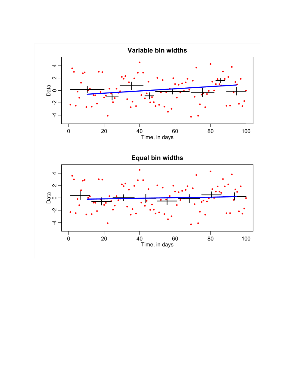
In Figure 1 we give a simple example of this kind of manipulation. A time series of data recorded over 100 days is Monte Carlo generated with a Normal distribution of zero mean and no trend (red points). However, we (wrongly) believe that the underlying model has trend with slope $0.02$ days^-1. Using varying bin widths from 5 to 20 days, we thus use Monte Carlo methods to determine the bin boundaries that yield a binned likelihood fitted trend that is most consistent with this mistaken hypothesis. The results are shown in Figure 1; the fitted slope with the optimized binning is $0.018\pm 0.006$, which is nicely consistent with the desired slope of $0.02$, and is three standard deviations away from the true slope of zero. However, if equal sized bins are employed, the likelihood fit returns a slope of $0.005\pm 0.007$, which is consistent with zero, and over two standard deviations away from the desired incorrect slope.

Thus, when given the freedom to chose variable bin widths and the placement of the bin boundaries, we see from just this one simple example that it is possible for researchers to accept a desired (but wrong) hypothesis, and reject the true hypothesis. In the following sections we will discuss a much more complicated example that involves fitting the phase of periodic data with carefully chosen variable bin widths. We will show that if empirical data exhibit annual modulation due to a true underlying phase, $\phi_{a}$, implementing variable width binning when fitting for the phase can unfortunately often result in an incorrect conclusion that the the data are instead consistent with a different phase, $\phi_{b}$.

Before moving on, we would like to stress that the manipulation of the data in this way, when it occasionally occurs, should not be assumed to be motivated by deliberate researcher prevarication; rather, such manipulations can happen when the researchers sincerely believe an incorrect model to be the true underlying description of their data, and thus wish to present the data in a way that highlights what they believe to be evidence of that relationship.

2 Methods

Here we consider an illustrative example with basis in the real world, simulating periodic data similar to that of a typical dark matter experiment[2]. Daily data with annual periodicity are simulated over a five year time span, with an annual variation of amplitude $A\sim 0.015$, and true phase $\phi_{a}$, which for illustrative purposes only we assume to be due to background or some other systematic effect. To simulate the observed data, $Y^{\rm obs}_{i}$, at day $t_{i}$, we thus use the model

$$Y^{\rm obs}_{i}=A\cos{2\pi(t_{i}-\phi_{A})}+\sigma_{a}{\cal N}(0,1),$$ (1)

where ${\cal N}(0,1)$ is random number drawn from the Normal distribution. For this example we assume the daily variation in the data is $\sigma_{a}\sim 0.05$.

We examine various binnings of the data, with bins between 30 days to 90 days in width. One thousand randomly selected binning schemes are examined, and the binning scheme is chosen that provides the best agreement of the fitted phase to the model

$$Y^{\rm pred}_{i}=A\cos{2\pi(t_{i}-\phi_{b})}\hskip 56.9055pt\phi_{b}\neq\phi_{a},$$ (2)

and worst agreement to the model with the true phase, $\phi_{a}$.

Using this unequal width binning scheme, we then perform a binned maximum likelihood fit to the data to obtain the estimated phase, $\hat{\phi}$, and its uncertainty, $\Delta\hat{\phi}$.

We compare this to the phase estimate of an unbinned likelihood fit, and we also examine the phase estimate of a binned likelihood fit with bins of equal width.

Here we arbitrarily assume that the phase of physics interest, $\phi_{b}$, is 90 days past January 1^st. We examine values of $\phi_{a}$ from 45 to 85 days past January 1^st, in steps of 5 days. Note that it doesn’t matter for this analysis what we assume for $\phi_{b}$, because the results only depend on the absolute difference between $\phi_{b}$ and $\phi_{a}$.

For each true phase value, $\phi_{a}$, we repeat the simulation and fitting procedure 250 times.

3 Results

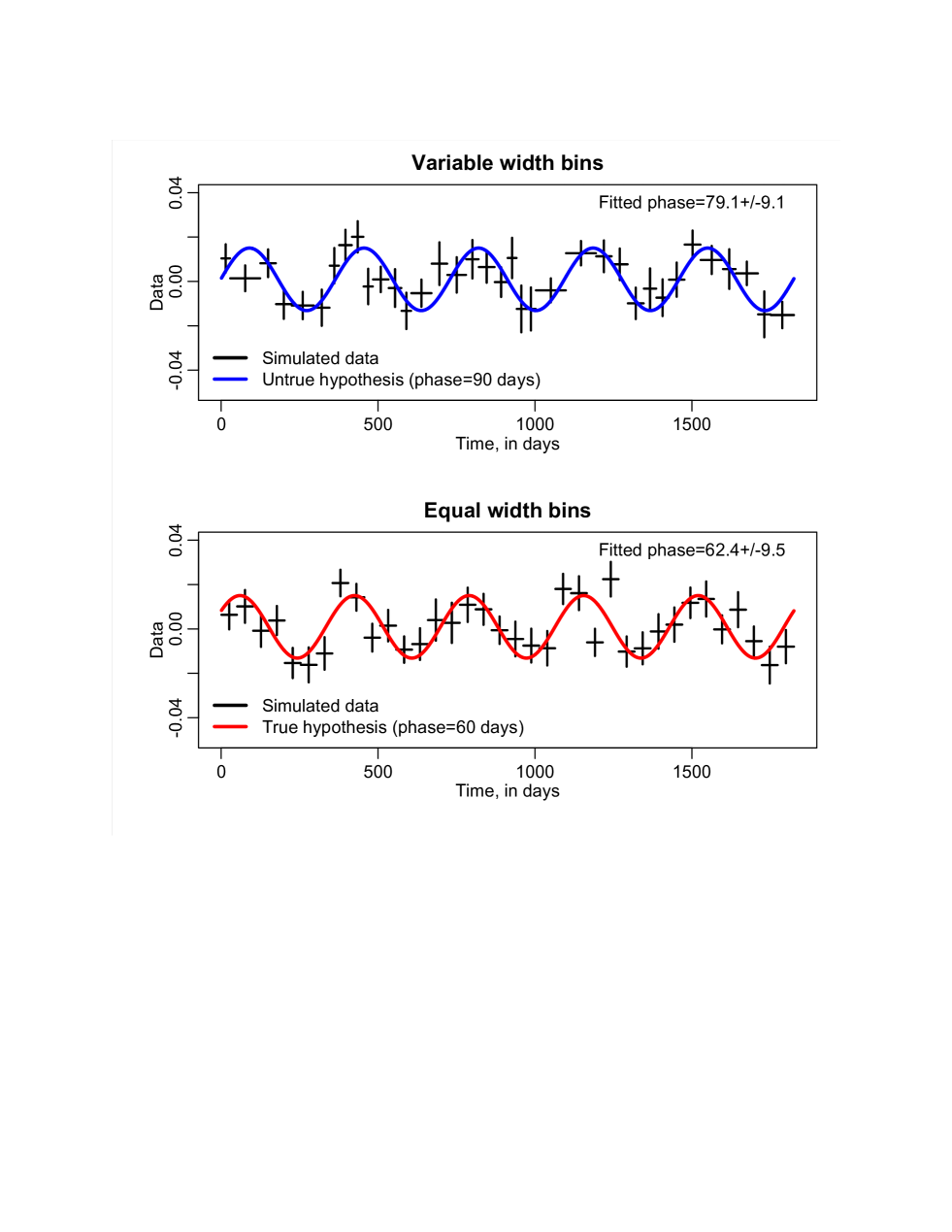
An example of the significant bias that can be achieved with variable width bins when fitting to the simulated harmonic data is shown in Figure 2. The true phase of the data is $\phi_{a}=60$ days and the variable width binning is tuned to best match a desired phase of $\phi_{b}=90$ days. The fit to the variably binned data yields an estimated phase, $\hat{\phi}=79.1\pm 9.1$, which is consistent with the untrue hypothesis, and statistically inconsistent with the true hypothesis. Conversely, fitting with the same number of equal sized bins (bottom plot in Figure 2) yields an estimate of the phase, $\hat{\phi}=62.4\pm 9.5$, which is statistically consistent with the true hypothesis and statistically inconsistent with the untrue hypothesis.

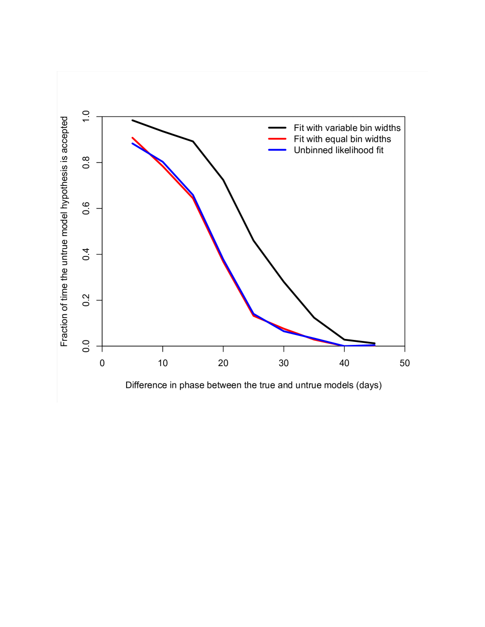
The results of using variable binning with 250 data simulations for various values of $\phi_{a}$ reveal that on average the variably binned fit yields a phase estimate that is around one standard deviation closer to the untrue hypothesis than the phase estimate from the unbinned and/or equal bin width fit. This results in the untrue phase hypothesis being accepted much more often than it would be if the fit is unbiased. For instance, as seen in Figure 3, when the true and untrue phase hypotheses are a month apart, using variable binning instead of unbinned or equal width binning more than triples the chances of accepting the untrue hypothesis as being correct (from 8% to 28%). For a three week phase difference, the fit with variable binning doubles the probability of accepting the untrue hypothesis from 37% to 73%. Indeed, as seen in the Figure, for all differences between the phase hypotheses, variable binning yields a significantly improved probability of accepting the untrue hypothesis.

4 Summary

We have shown that fitting to data grouped into bins of variable widths can yield significantly biased results. Using a simple example of linear data, and a much more complicated example of periodic data, we have shown that fitting with variable binning can too often produce biased estimates that result in an incorrect model hypothesis being accepted as true. In the cases examined, we have shown that unbinned likelihood fits and/or binned fits with bins of equal width produce unbiased results.

The examples given in this paper are illustrative only, and certainly not an exhaustive examination of the degree of bias that can be obtained in any particular physics analysis when variable width binning is employed. Researchers must thus be careful to employ variable bin widths only when absolutely necessary, and reviewers must be careful to inquire about the underlying motivation when reviewing a fitting analysis wherein the bin widths are variable. The only truly reliable cross-check of sensitivity to binning effects is to fit with equal width bins or, ideally, perform an unbinned likelihood fit. It is not enough for researchers to merely state that “alternate” binning schemes were examined, since the alternate binning schemes may have been chosen to be different, but still nevertheless quite optimal in affirming the desired (but wrong) hypothesis.

Figure 1: As an example of the significant biases that can result when fitting with variable width bins, data are generated over 100 days, sampling from a Normal distribution, with no trend (red points). The top plot shows the fit when variable width bins are employed to optimize the agreement with the grouped data (black points) to a model that assumes the slope is $0.02$ days^-1. The fit returns an estimated slope of $0.018\pm 0.006$, which is three standard deviations from the true value. The bottom plot shows the fit to the data grouped into bins of equal width. The fit yields an estimated slope of $0.005\pm 0.007$, consistent with the true value.

Figure 2: As another example of the significant biases that can result when fitting with variable width bins, we fit to simulated data with an annual harmonic variation with true phase $\phi_{a}=60$ days (relative to January 1^st). In the upper plot, variable binning is used to obtain the best comparison to an incorrect model with phase $\phi_{b}=90$ days. The fit to the variably binned data yields an estimated phase consistent with this untrue hypothesis, and statistically inconsistent with the true hypothesis. Conversely, fitting with equal sized bins (bottom plot) yields an estimate of the phase that is statistically consistent with the true hypothesis, and statistically inconsistent with the untrue hypothesis. The Pearson $\chi^{2}$ statistics for the upper and lower plots are $29$ and $40$, with 34 degrees of freedom, respectively.

Figure 3: For simulated data with annual periodicity, we examine 250 trials for true phase values, $\phi_{a}$, that differ from a desired phase hypothesis, $\phi_{b}$, by various amounts between 5 to 45 days. The blue line shows the results achieved when an unbinned likelihood fit is employed. The red line shows the results of a binned likelihood fit with bins of equal width. Both types of fits yield values of $\phi_{a}$ that are unbiased. The black line shows the results achieved with a binned likelihood fit with bins of varying width, where the bin boundaries are chosen to optimize agreement with the untrue phase hypothesis, $\phi_{b}$. The fits with variable bin widths produce significantly biased results that cause us to too often conclude the data are consistent with the untrue hypothesis.

References

- [1] Babbage, C (1830) Reflections on the Decline of Science in England, and on Some of Its Causes, B. Fellowes, publisher (Republished by Gregg International in 1969, London)
- [2] Hasenbalg, F (1998) Annual modulation sensitivity in cold dark matter searches. Astroparticle Physics, 9: 339-347.