The Effect of Curvaton Decay on the Primordial Power Spectrum

Abstract

We study the effect of curvaton decay on the primordial power spectrum. Using analytical approximations and also numerical calculations, we find that the power spectrum is enhanced during the radiation dominated era after the curvaton decay. The amplitude of the Bardeen potential is controlled by the fraction of the energy density in the curvaton at the time of curvaton decay. We show that the enhancement in the amplitude of the primordial curvature perturbation is, however, not large enough to lead to primordial black hole overproduction on scales which re-enter the horizon after the time of curvaton decay.

I Introduction

Recent results from experiments at the LHC in Geneva give a very strong indication of the existence of a Higgs like particle. If confirmed, this would be the first observation of a scalar field outside cosmology. For many years scalar fields have been nearly indispensable in theoretical cosmology, not only in solving many problems of the hot big bang model, but also in generating the primordial power spectrum of density fluctuations (see e.g. Ref. LL ).

The curvaton scenario Lyth:2001nq ; Enqvist:2001zp ; Moroi:2001ct is an elegant extension to the standard inflation scenario. Whereas in the standard scenario the fields driving inflation and the field generating the primordial power spectrum are the same, in the curvaton scenario these tasks are performed by two (or more) fields. While the inflaton field drives inflation, the curvaton field is a mere spectator field (massless or nearly massless), picking up a nearly scale invariant spectrum during inflation. After inflation the inflaton field decays into radiation and the curvaton behaves like dust, oscillating around the minimum of its potential. After this brief matter dominated period the curvaton also decays into radiation. Due to its simplicity and elegance the curvaton scenario has enjoyed widespread attention in recent years (see e.g. Refs. Bartolo:2002vf ; Lyth:2002my ; Lyth:2003ip ; Dimopoulos:2003ss ; Bartolo:2003jx ; Malik:2006pm ; Sasaki:2006kq ; Assadullahi:2007uw ; Enqvist:2008be ; Dimopoulos:2012nj ; Assadullahi:2012yi .

In most standard curvaton calculations the power spectrum of the curvature perturbation $\zeta$ (the quantity that later on sources the CMB and LSS) is assumed to be directly inherited from the curvaton field. In this paper we study in detail the effect of curvaton decay on the primordial power spectrum. In particular we investigate whether the change in the initial power spectrum on small scales can lead to primordial black hole (PBH) production. To keep our results as general as possible, we do not specify a potential for the curvaton field, assuming only that it oscillates around the minimum of its potential, and hence behaves like dust, before decaying into radiation.

The outline of the paper is as follows. In Sections II and III we present the equations governing the background and perturbation evolution. In Section IV we derive analytical approximations for the Bardeen potential, and calculate the effect of curvaton decay on the power spectrum of $\zeta$. We then calculate the abundance of PBHs formed in Section V. We conclude with a brief discussion in the final section.

II Background Dynamics

In this section we provide the background dynamics. We consider two interacting fluids in a Friedmann-Robertson-Walker (FRW) universe: radiation with equation of state $P\equiv\omega_{\rm r}\rho_{\rm r}$, where $\omega_{\rm r}=1/3$ and the curvaton with dust like equation of state. We assume the inflaton entirely decays into radiation at the end of inflation. Initially radiation dominates and the curvaton energy density is very sub-dominant. We assume that the curvaton decays into radiation with a constant decay rate $\Gamma$ when the Hubble expansion rate $H$ drops below $\Gamma$.

II.1 Background Equations

The continuity equations for each individual fluid in the background can be written as wands1 ; wands2

$$\dot{\rho}_{\sigma}+3H\rho_{\sigma}=-\Gamma\rho_{\sigma}\,,$$ (1)

$$\dot{\rho}_{r}+4H\rho_{r}=\Gamma\rho_{\sigma}\,,$$ (2)

where $\rho_{\sigma}$ and $\rho_{\rm r}$ are the background energy density of the curvaton and radiation respectively and a dot indicates the derivative with respect to cosmic time $t$. The right-hand side of equations (1) and (2) describe the background energy transfer per unit time from the curvaton and to the radiation fluid respectively. The Hubble parameter $H$ is determined by the Friedmann constraint

$$H^{2}=\frac{1}{3\,M^{2}_{\rm{Pl}}}\>(\rho_{\sigma}+\rho_{r})\,,$$ (3)

where $M_{\rm{Pl}}\equiv 1/\sqrt{8\pi G}$ is the reduced Planck mass. In order to obtain the evolution of the above dynamical system, it is useful to write the equations in terms of dimensionless parameters

$$\Omega_{\sigma}=\frac{\rho_{\sigma}}{\rho},\>\>\>\>\>\>\textrm{and}\>\>\>\>\>\Omega_{r}=\frac{\rho_{r}}{\rho}\,,$$ (4)

where

$$\sum_{\alpha}\rho_{\alpha}=\rho\,,$$ (5)

is the total energy density and hence $\Omega_{\sigma}+\Omega_{r}=1$. One can easily derive the following evolution equations for these dimensionless parameters:

$$\Omega^{{}^{\prime}}_{\,\sigma}(N)-\Omega_{\,\sigma}(N)\Omega_{\,r}(N)+\frac{\Gamma}{H(N)}\,\Omega_{\,\sigma}(N)=0\,,$$ (6)

$$\Omega^{{}^{\prime}}_{\,r}(N)+\Omega_{\,r}(N)\Omega_{\sigma}(N)-\frac{\Gamma}{H(N)}\,\Omega_{\,\sigma}(N)=0\,,$$ (7)

$$H^{{}^{\prime}}(N)+\frac{3}{2}H(N)+\frac{1}{2}H(N)\Omega_{\,r}(N)=0\,,$$ (8)

where a prime denotes differentiation with respect to the number of e-folding $N\equiv\int H\textrm{d}t$. We set $N=0$ at the end of reheating.

II.2 Sudden decay limit

Useful intuition can be gained by first considering the analytical solutions of the system of Eqs. (6–8) in the sudden decay limit where $\Gamma=0$. This is a good approximation until the time of curvaton decay at $N=N_{\rm d}$ when $\Gamma\sim H$ and the curvaton decays to radiation. In the sudden decay limit where $\Gamma/H=0$, Eqs. (6), (7) and (8) can be solved easily for the background quantities $\Omega_{\rm r}(N),\Omega_{\sigma}(N)$, and $H(N)$, to obtain

$$\Omega_{\rm r}(N) = \frac{1}{1+p\,e^{N}}\,,$$ (9)

$$\Omega_{\sigma}(N) = \frac{p\,e^{N}}{1+p\,e^{N}}\,,$$ (10)

$$H(N) = H_{0}e^{-2N}\left(1+p\,e^{N}\right)^{1/2}\,,\quad$$ (11)

where $H_{0}$ is the value of $H$ at the start of radiation dominated epoch, after the end of reheating, when $N=0$. Here we have defined the ratio $p$

$${p}\equiv\frac{\Omega_{\sigma\,{\rm in}}}{\Omega_{{\rm r}\,{\rm in}}}\,,$$ (12)

where $\Omega_{\sigma\,{\rm in}}$ and $\Omega_{{\rm r}\,{\rm in}}$ are the initial values of $\Omega_{\sigma}$ and $\Omega_{\rm r}$ at the end of reheating, so that if radiation initially dominates $p\ll 1$.

A key parameter in curvaton analysis is $f_{\rm d}$, the weighted fraction of curvaton energy density to the total energy density at the time of curvaton decay, defined by

$$f_{\rm d}\equiv\frac{3\rho_{\sigma}}{3\rho_{\sigma}+4\rho_{r}}{\big{|}}_{\mathrm{dec}}=\frac{3\Omega_{\sigma}}{4-\Omega_{\sigma}}{\big{|}}_{\mathrm{dec}}\sim\Omega_{\sigma}|_{\mathrm{dec}}\,.$$ (13)

As is well-known Lyth:2001nq ; Lyth:2002my , the non-Gaussianity parameter $f_{\rm NL}$ on CMB scales is approximately given by $f_{\rm NL}\sim 1/f_{\rm d}$. In Section IV we find the Bardeen potential $\Psi$ for various limiting values of $f_{\rm d}$.

II.3 Beyond the sudden decay limit

Here we provide solutions for $\Omega_{\rm r}(N)$ and $\Omega_{\sigma}(N)$ which can also be used after the time of curvaton decay. Comparison with the full numerical solution to Eqs. (6–8) shows that while our analytical solution for $H(N)$ in the sudden decay limit, Eq. (11) is in reasonable agreement with the numerical solution the analytical sudden decay solutions for $\Omega_{\rm r}(N)$ and $\Omega_{\sigma}(N)$, Eqs. (9) and (10), are not accurate for $N>N_{\rm d}$ as expected. This indicates that more accurate analytical solutions for $\Omega_{\rm r}(N)$ and $\Omega_{\sigma}(N)$ can be found by inserting the solution for $H(N)$ into Eqs. (6) and (7) and then solving for $\Omega_{\rm r}(N)$ and $\Omega_{\sigma}(N)$.

Defining

$$X\equiv\frac{\Omega_{\sigma}}{\Omega_{r}}\,,$$ (14)

from Eqs. (6) and (7) we find

$$X^{\prime}=X-\frac{\Gamma}{H}(1+X)X\,,$$ (15)

with $H(N)$ given by Eq. (11). It is not possible to solve Eq. (15) in general. However, away from the time of curvaton decay, we have $X<1$, i.e. $\Omega_{\sigma}<\Omega_{\rm r}$ so Eq. (15) can be approximated by a linear differential equation which can be solved analytically yielding

$$X \simeq p\exp{\left[\int_{0}^{N}{\rm d}N^{\prime}\left(1-\frac{\Gamma}{H(N^{\prime})}\right)\right]}\,,$$ (16)

$$\simeq p\exp\left\{-\frac{2\Gamma}{H_{0}p^{2}}\left[\sqrt{1+pe^{N}}\left(\frac{1+pe^{N}}{3}-1\right)+\frac{2}{3}\right]+N\right\}\,.$$ (17)

In the integrand above $H(N^{\prime})$ is calculated from the sudden decay limit solution given in Eq. (11). Correspondingly

$$\Omega_{r}(N)=\frac{1}{1+X}\quad,\quad\Omega_{\sigma}(N)=\frac{X}{1+X}\,.$$ (18)

Note that before the time of curvaton decay when one can neglect the last term in Eq. (15) and $X\simeq pe^{N}$, Eq. (18) reduces to Eqs. (9) and (10) obtained in the sudden decay limit.

For the physically interesting case in which the curvaton makes a sub-dominant contribution to the total energy density at the time of decay, corresponding to $\Omega_{\sigma}|_{\rm dec}\ll 1$, one can take $\Omega_{\sigma}(N)\ll\Omega_{\rm r}(N)$ throughout the whole evolution and to a good approximation $H(N)$ is given, as in a radiation dominated Universe, by $H(N)\simeq H_{0}e^{2N}$. Inserting this expression for $H$ into Eq. (16) yields

$$\Omega_{\sigma}\simeq p\exp\left(N-\frac{\Gamma}{2H_{0}}e^{2N}\right)\,,\quad\Omega_{r}=1-\Omega_{\sigma}\,,\quad\quad\quad\quad\left(f_{\rm d}\ll 1\right)\,.$$ (19)

In Fig. 1 we have plotted the full numerical solutions for $\Omega_{\sigma}(N)$ and $\Omega_{\rm r}(N)$ and compared them with our analytical solutions Eqs. (18) and (19). As can be seen, for small values of $\Omega_{\sigma}|_{\mathrm{dec}}$, or equivalently small values of $f_{\rm d}$, the agreement between our analytical solutions and the full numerical solutions is very good.

Finally we obtain an estimate for $N_{\rm d}$, the time of curvaton decay. A good criteria to define $N_{\rm d}$ in the sudden decay limit is when the last term in Eq. (15) becomes comparable to the second term and $X^{\prime}(N_{\rm d})=0$, and the ratio $\Omega_{\sigma}/\Omega_{\rm r}$ reaches its maximum. This gives $\Gamma(1+X(N_{\rm d}))=H(N_{\rm d})$. In the limit where $X(N_{\rm d})\ll 1$, or equivalently $f_{\rm d}\ll 1$, this reduces to the standard result that $H(N_{\rm d})\simeq\Gamma$ or

$$N_{\rm d}\simeq\frac{1}{2}\ln\left(\frac{H_{0}}{\Gamma}\right)\,,\quad\quad\quad\quad\left(f_{\rm d}\ll 1\right)\,.$$ (20)

Inserting this expression for $N_{\rm d}$ into the definition of $f_{\rm d}$ in Eq. (13) yields

$$f_{\rm d}\sim\frac{3p}{4}\left(\frac{H_{0}}{\Gamma}\right)^{1/2}\,,\quad\quad\left(f_{\rm d}\ll 1\right)\,.$$ (21)

In general, when $f_{\rm d}\gtrsim 1/2$ then Eq. (20) receives corrections and one has to find $N_{\rm d}$ by solving $X^{\prime}=0$ with $X$ given by Eq. (17).

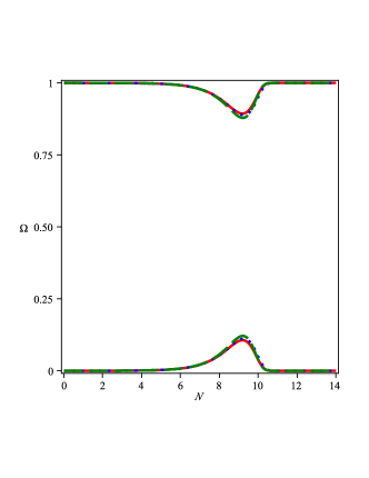
Figure 1: The evolution of $\Omega_{\rm r}$ and $\Omega_{\sigma}$ for $\Gamma/H_{0}=10^{-8}$. The left panel is for $f_{\rm d}$, the weighted ratio of the curvaton energy density to the total energy density at the time of curvaton decay, equal to $0.08$ and the right panel for $f_{\rm d}=0.16$. In each plot, the upper curves are $\Omega_{\rm r}$ while the lower curves are $\Omega_{\sigma}$. The solid red curves are the full numerical solution, the blue dotted curves the analytic solutions, Eqs. (18), and the green dashed curves the analytic solutions in the $f_{\rm d}\ll 1$ limit, Eqs. (19). As expected, for small values of $f_{\rm d}$ the agreement between the numerical and the analytical solutions is very good.

III Perturbations

In this section we study the perturbed Einstein and fluid equations. The perturbed metric line element is Mukhanov:1990me ; Malik:2004tf ; Malik:2008im

$${\rm d}s^{2}=-(1+2\phi){\rm d}t^{2}+2aB_{,i}{\rm d}t{\rm d}x^{i}+a^{2}\left[(1-2\psi)\delta_{ij}+2E_{,ij}\right]{\rm d}x^{i}{\rm d}x^{j}\,.$$ (22)

The perturbed Einstein equations are then

$$\Psi^{\prime}+\frac{5+3\omega}{2}\Psi+\frac{k^{2}}{3a^{2}H^{2}}\Psi+\frac{3}{2}(1+\omega)\zeta=0\,,$$ (23)

and

$$\Psi^{\prime}+\frac{5+3\omega}{2}\Psi-\frac{3}{2}(1+\omega){\cal R}=0\,,$$ (24)

where the time-dependent equation of state $w$ is given by

$${w}\equiv\frac{P}{\rho}=\sum_{\alpha}\frac{\omega_{\alpha}\,\rho_{\alpha}}{\rho}\,,$$ (25)

in which $\omega_{\alpha}$ is the equation of state for each fluid given by $\omega_{\alpha}=p_{\alpha}/\rho_{\alpha}$ with $\omega_{\sigma}=0$ and $\omega_{r}=1/3$.

Here we have defined the Bardeen potential, or curvature perturbation on uniform shear hypersurfaces, as

$$\Psi\equiv\psi-H(B-\dot{E})\,,$$ (26)

and the curvature perturbations on uniform density slices $\zeta$, and on comoving hypersurfaces, ${\cal R}$, respectively as

$$\zeta\equiv-\psi-\frac{H\delta\rho}{\dot{\rho}}\,,\qquad{\cal R}\equiv\psi-HV\,,$$ (27)

where $V\equiv a(v+B)$, and $v$ is the total scalar velocity potential.

Equations (23) and (24) can be combined to give

$$\frac{k^{2}}{3a^{2}H^{2}}\Psi=-\frac{3}{2}(1+\omega)(\zeta+{\cal R})\,.$$ (28)

In particular, we see that on large scale where $k/aH\rightarrow 0$, $\zeta\simeq-{\cal R}$.

The equations of motion for each fluid are

$$\delta\rho_{\alpha}^{\prime}+3(\delta\rho_{\alpha}+\delta p_{\alpha})-3(\rho_{\alpha}+p_{\alpha})\psi^{\prime}-\frac{k^{2}}{a^{2}H}(\rho_{\alpha}+p_{\alpha})(V_{\alpha}+\sigma_{s})-\frac{1}{H}(Q_{\alpha}\phi+\delta Q_{\alpha}) = 0\,,$$ (29)

$$V^{\prime}_{\alpha}+\left[\frac{Q_{\alpha}}{H(\rho_{\alpha}+p_{\alpha})}(1+c_{\alpha}^{2})-3c_{\alpha}^{2}\right]V_{\alpha}+\frac{\phi}{H}+\frac{1}{H(\rho_{\alpha}+p_{\alpha})}\left[\delta p_{\alpha}-Q_{\alpha}V\right] = 0\,,$$ (30)

where the sound speed for each fluid is defined by $c_{\alpha}^{2}=\dot{p}_{\alpha}/\dot{\rho}_{\alpha}$. We shall assume further below that each fluid is intrinsically adiabatic so $p_{\alpha}=p_{\alpha}(\rho_{\alpha})$ and $\delta p_{\alpha}=c_{\alpha}^{2}\delta\rho_{\alpha}$. Also $v_{\alpha}$ is the scalar velocity potential for each fluid and $V_{\alpha}\equiv a(v_{\alpha}+B)$.

In order to express the fluid equations, Eqs. (29) and (30), in gauge invariant form, we define the curvature perturbations $\zeta_{\alpha}$ and ${\cal R}_{\alpha}$ for each fluid as

$$\zeta_{\alpha}\equiv-\psi-H\frac{\delta\rho_{\alpha}}{\dot{\rho}_{\alpha}}\,,$$ (31)

and

$${\cal R}_{\alpha}\equiv\psi-HV_{\alpha}\,.$$ (32)

One can cast the perturbed fluid equations, Eqs. (29) and (30), into Malik:2004tf

$$\zeta_{\alpha}^{\prime}=-\frac{H^{\prime}Q_{\alpha}}{H^{2}\rho_{\alpha}^{\prime}}\left(\frac{\delta\rho_{\alpha}}{\rho_{\alpha}^{\prime}}-\frac{\delta\rho}{\rho^{\prime}}\right)-\frac{1}{H\rho_{\alpha}^{\prime}}\left(\delta Q_{\alpha}-\frac{Q_{\alpha}^{\prime}}{\rho_{\alpha}^{\prime}}\delta\rho_{\alpha}\right)+\frac{k^{2}}{3a^{2}H^{2}}\left[\Psi-\left(1-\frac{Q_{\alpha}}{H\rho_{\alpha}^{\prime}}\right){\cal R_{\alpha}}\right]\,,$$ (33)

and

$${\cal R}_{\alpha}^{\prime}=\left(\frac{Q_{\alpha}}{H(\rho_{\alpha}+p_{\alpha})}-\frac{H^{\prime}}{H}\right)\left({\cal R}-{\cal R}_{\alpha}\right)-\frac{\rho_{\alpha}^{\prime}}{\rho_{\alpha}+p_{\alpha}}c_{\alpha}^{2}\left({\cal R}_{\alpha}+\zeta_{\alpha}\right)\,.$$ (34)

In the absence of energy transfer between the fluids, $Q_{\alpha}=\delta Q_{\alpha}=0$, we see that $\zeta_{\alpha}$ for each fluid is constant on super-horizon scales Wands:2000dp . Note that in deriving Eqs. (33) and (34) we have assumed that each fluid is intrinsically adiabatic so $p_{\alpha}=p_{\alpha}(\rho_{\alpha})$ and $\delta p_{\alpha}=c_{\alpha}^{2}\delta\rho_{\alpha}$.

We also note that $\zeta$ and ${\cal R}$ defined in Eq. (27) can be written as the weighted sum of $\zeta_{\alpha}$ and ${\cal R}_{\alpha}$,

$$\zeta=\sum_{\alpha}\frac{\dot{\rho}_{\alpha}}{\dot{\rho}}\zeta_{\alpha}=\sum_{\alpha}\frac{(1+\omega_{\alpha})\rho_{\alpha}}{(1+\omega)\rho}{\zeta}_{\alpha}\,,$$ (35)

and

$${\cal R}=\sum_{\alpha}\frac{(1+\omega_{\alpha})\rho_{\alpha}}{(1+\omega)\rho}{\cal R}_{\alpha}\,.$$ (36)

So far we have not specified the perturbations in the energy transfer $\delta Q_{\alpha}$. Following Ref. wands1 , we assume that the decay rate $\Gamma$ is fixed by the microphysics so $\delta\Gamma=0$ and therefore

$$\delta Q_{\sigma}=-\Gamma\delta\rho_{\sigma}\,,\quad\delta Q_{\gamma}=\Gamma\delta\rho_{\sigma}\,.$$ (37)

The system of equations in terms of $\{\zeta_{\sigma},{\cal R}_{\sigma},\zeta,{\cal R}\}$ is given by

$$\zeta_{\sigma}^{\prime} = \frac{(3+\Omega_{\gamma})\Gamma}{2(\Gamma+3H)}(\zeta-\zeta_{\sigma})+\frac{k^{2}}{3a^{2}H^{2}}\Psi-\frac{k^{2}}{a^{2}H^{2}}\left(\frac{H}{3H+\Gamma}\right){\cal R}_{\sigma}\,,$$ (38)

$$\zeta^{\prime} = \frac{(\Gamma+3H)\Omega_{\sigma}}{H(3+\Omega_{\gamma})}(\zeta_{\sigma}-\zeta)+\frac{k^{2}}{3a^{2}H^{2}}(\Psi-{\cal R})\,,$$ (39)

$${\cal R}_{\sigma}^{\prime} = -\left(\frac{\Gamma}{H}+\frac{H^{\prime}}{H}\right)\left({\cal R}-\frac{3(1+\Omega_{\gamma})}{3+\Omega_{\sigma}}{\cal R}_{\sigma}\right)\,,$$ (40)

$${\cal R}^{\prime} = \left(\frac{H^{\prime}}{H}+\frac{4H\Omega_{\gamma}-\Gamma\Omega_{\sigma}}{H(3+\Omega_{\gamma})}\right){\cal R}+\left(1+\frac{H^{\prime}}{H}\right)\zeta-\frac{(\Gamma+3H)\Omega_{\sigma}}{H(3+\Omega_{\gamma})}\zeta_{\sigma}-\frac{k^{2}}{3a^{2}H^{2}}\Psi\,.$$ (41)

Note that this is a closed system of equation for $\{\zeta_{\sigma},{\cal R}_{\sigma},\zeta,{\cal R}\}$ and that $\Psi$ can be eliminated from these equations using Eq. (28) in terms of $\zeta$ and ${\cal R}$.

Alternatively, one may write the system of equations in terms of $\{\zeta_{\rm r},{\cal R}_{\rm r},\zeta,{\cal R}\}$ or $\{\zeta_{\rm r},{\cal R}_{\rm r},\zeta_{\sigma},{\cal R}_{\sigma}\}$ as given in Appendix A.

IV Analytic Calculation of Bardeen potential

In this section we provide the analytical solutions for the Bardeen potential $\Psi$ in different limits. As can be seen, the system of Eqs. (38)-(41) is too complicated to be handled analytically for all modes. However analytical solutions for $\Psi$ can be obtained in some limiting situations. In the next two subsections we consider modes which are super-horizon at the time of curvaton decay, $k<a(N_{d})H(N_{d})$, and modes which are always sub-horizon during curvaton evolution corresponding to $k>H_{0}$ where $H_{0}$ is the Hubble constant at the end of reheating when $a(N=0)=1$.

IV.1 Super-horizon modes

Here we provide the solution for the modes which are super-horizon at the time of curvaton decay and re-enter the horizon during the second radiation stage. First we consider the epoch before the curvaton decays, $N<N_{\rm d}$. In the sudden decay limit, for the super-horizon modes from Eqs. (74) and (75) it can be shown that $\zeta_{\rm r}^{\prime}\simeq 0$ and $\zeta_{\sigma}^{\prime}\simeq 0$. As expected, on super-horizon scales both $\zeta_{\sigma}$ and $\zeta_{\rm r}$ remain frozen so one can approximate $\zeta_{\sigma}$ with its value at the time of horizon crossing during inflation

$$\zeta_{\sigma}(N)\simeq\zeta_{\sigma_{*}}\,.$$ (42)

Also to further simplify the analysis, we consider the conventional curvaton mechanism where $\zeta_{\gamma\,{\rm in}}=0$ and there is no initial radiation perturbation, corresponding to entropic initial conditions. In this limit, either by solving Eq. (80) or using the definition (35), we have

$$\zeta=\frac{3\Omega_{\sigma}}{4-\Omega_{\sigma}}\zeta_{\sigma_{*}}\,.$$ (43)

Substituting this into Eq. (23) and noting that $w=\Omega_{\rm r}(N)/3$ and using Eq. (11), results in

$$\Psi^{\prime}+\frac{1}{2}\left(5+\frac{1}{1+p\,e^{N}}\right)\Psi+\frac{3p\,e^{N}\zeta_{\sigma_{*}}}{2(1+p\,e^{N})}=0\,.$$ (44)

This can easily be solved with the result

$$\Psi(N)=\left[C\,\sqrt{1+p\,e^{N}}-\frac{3\zeta_{\sigma_{*}}}{5p^{3}}\left(16+8p\,e^{N}-2p^{2}\,e^{2N}+p^{3}e^{3N}\right)\right]e^{-3N}\,.$$ (45)

Here $C$ is a constant of integration which is obtained by matching this solution to the value of $\Psi$ at the end of inflation, which gives

$$C=\frac{1}{\sqrt{1+p}}\left[\Psi(0)+\frac{3\zeta_{\sigma_{*}}}{5p^{3}}\left(16+8p-2p^{2}+p^{3}\right)\right]\,\simeq\frac{48\zeta_{\sigma_{*}}}{5p^{3}}\,.$$ (46)

To obtain the second approximate relation we used $p\ll 1$ and $\Psi(0)\simeq 0$ which is a good approximation for all modes at the end of inflation Lyth:2005ze .

Having obtained $\Psi$ during curvaton evolution, we now find $\Psi$ after the curvaton decays. The governing equation for $\Psi$ during the radiation domination stage with $\omega_{\rm r}=1/3$ has the standard form

$$\Psi^{\prime\prime}+3\Psi^{\prime}+\frac{k^{2}}{3a^{2}H^{2}}\Psi=0\,.$$ (47)

Using

$$H=H_{{\rm d}}e^{-2(N-N_{{\rm d}})}\,,$$ (48)

during the radiation era this leads to a solution in terms of Bessel functions,

$$\Psi(N)=e^{-3N/2}\left[c_{1}J_{3/2}\left(\bar{k}e^{N}\right)+c_{2}Y_{3/2}\left(\bar{k}e^{N}\right)\right]\,,$$ (49)

in which $c_{1}$ and $c_{2}$ are two constants of integration and

$$\bar{k}\equiv\frac{ke^{-2N_{{\rm d}}}}{\sqrt{3}H_{\rm d}}\,.$$ (50)

In the limit where the curvaton makes a sub-dominant contribution to the total energy density at the time of decay, corresponding to $f_{\rm d}\ll 1$, one can use Eqs. (11) and (20) to obtain $H_{\rm d}\simeq\Gamma$ and $\bar{k}\sim k/H_{0}$. Also the condition for the mode $k$ to be superhorizon at the time of curvaton decay, $k>H_{\rm d}e^{N_{\rm d}}$, translates into $k>\sqrt{\Gamma H_{0}}$.

We can now determine the constants of integration $c_{1}$ and $c_{2}$, by requiring that both $\Psi$ and $\Psi^{\prime}$ are continuous at the time of curvaton decay, $N=N_{d}$. This gives

$$c_{1} = \frac{\pi}{2}\left[\left(\bar{k}e^{5N_{\rm d}/2}Y^{\prime}_{3/2}(\bar{k}e^{N_{\rm d}})-\frac{3}{2}e^{3N_{\rm d}/2}Y_{3/2}(\bar{k}e^{N_{\rm d}})\right)\Psi(N_{\rm d})-e^{3N_{\rm d}/2}Y_{3/2}(\bar{k}e^{N_{\rm d}})\Psi^{\prime}(N_{\rm d})\right]\,,$$ (51)

$$c_{2} = \frac{\pi}{2}\left[\left(-\bar{k}e^{5N_{\rm d}/2}J^{\prime}_{3/2}(\bar{k}e^{N_{\rm d}})+\frac{3}{2}e^{3N_{\rm d}/2}J_{3/2}(\bar{k}e^{N_{\rm d}})\right)\Psi(N_{\rm d})+e^{3N_{\rm d}/2}J_{3/2}(\bar{k}e^{N_{\rm d}})\Psi^{\prime}(N_{\rm d})\right]\,.$$ (52)

Note that in the above expressions $\Psi(N_{\rm d})$ and $\Psi^{\prime}(N_{\rm d})$ are calculated from the solution obtained from the period before the curvaton decay, Eq. (45).

By construction, we know that $a(N_{\rm d})H(N_{\rm d})<k$, so $\bar{k}e^{N_{\rm d}}\sim ke^{-N_{\rm d}}/H_{\rm d}<1$. Using the small argument limits of the Bessel functions we find that $c_{2}\ll c_{1}$ and therefore

$$\Psi(N)\simeq c_{1}e^{-3N/2}J_{3/2}(\bar{k}e^{N})\,,\quad(N\geq N_{d})\,.$$ (53)

Now suppose these modes (with $\bar{k}e^{N_{\rm d}}<1$) re-enter the horizon during the second radiation era at the time $N=N_{k}$. The value of $N_{k}$ can be estimated by calculating when the argument of the Bessel function in Eq. (53) becomes of order unity and $J_{3/2}(\bar{k}e^{N})$ starts to oscillate. This yields $\bar{k}e^{N_{k}}=1$ or $N_{k}=-\ln\bar{k}$. During the period $N_{d}<N<N_{k}$ in which the mode is still super-horizon during the second radiation stage we can use the small argument limit of the Bessel function $J_{\nu}(x)\simeq(x/2)^{\nu}/\Gamma(\nu+1)$ (here $\Gamma(\nu+1)$ is the gamma-function) to obtain

$$\Psi(N)\simeq\frac{c_{1}}{\Gamma(5/2)}\left(\frac{\bar{k}}{2}\right)^{3/2}\,,\quad N_{d}\leq N<N_{k}\,.$$ (54)

This is a very interesting result; for $N_{\rm d}<N<N_{k}$, $\Psi$ is constant with the value given by Eq. (54). Numerical evolution of $\Psi$, shown in Fig. 2, verifies the existence of this plateau.

During the epoch $N>N_{k}$, after the mode $k$ has re-entered the horizon, the Bessel function in Eq. (53) oscillates rapidly. Using the large argument limit of the Bessel function we obtain

$$\Psi(N)\simeq\sqrt{\frac{2}{\pi\bar{k}}}e^{-2N}c_{1}\,\cos\left(\bar{k}e^{N}+\frac{\pi}{4}\right)\,\,,\quad(N>N_{k})\,.$$ (55)

As we shall see in the following section in order to study whether PBHs are overproduced, we need to estimate $\Psi(N_{\rm d})$ and $c_{1}$. As mentioned before, the key parameter in controlling the amplitude of $\Psi(N)$ during the second radiation era is $f_{\rm d}$. Here we calculate $c_{1}$ for two extreme cases (i): $f_{\rm d}\ll 1$ corresponding to $pe^{N_{\rm d}}\ll 1$ and (ii): $f_{\rm d}\gtrsim 1/2$ corresponding to $pe^{N_{\rm d}}\ll 1$.

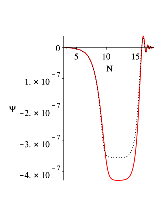
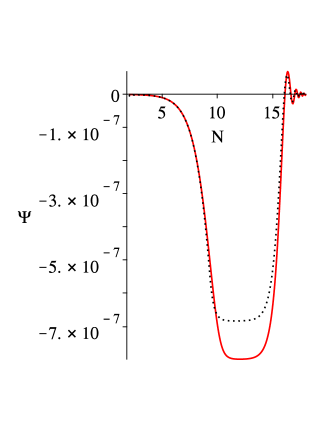
Figure 2: The evolution of the Bardeen potential $\Psi$ for super-horizon modes with $f_{\rm d}=0.08$ and $0.16$ (left and right plots respectively). In both plots $\Gamma/H_{0}=10^{-8}$ and the red curve is the full numerical result while the black dotted curve is our analytical solution, Eq. (49). In both plots, the existence of the plateau, Eq. (54), for the modes in the range $N_{\rm d}<N<N_{k}$ is evident. As expected from Eq. (58), the larger $f_{\rm d}$ is, the larger the amplitude of $\Psi$ is.

For the limit $f_{\rm d}\ll 1$, from Eq. (45) we obtain

$$\Psi(N_{\rm d})\simeq-\frac{3}{8}pe^{N_{\rm d}}\zeta_{\sigma_{*}}\simeq-\frac{f_{\rm d}}{2}\zeta_{\sigma_{*}}\,,\quad(f_{\rm d}\ll 1)\,,$$ (56)

where to obtain the second approximation, Eqs. (20) and (21) have been used. Similarly, using Eq. (44) to eliminate $\Psi^{\prime}$ we obtain

$$\Psi^{\prime}(N_{\rm d})\simeq-\frac{f_{\rm d}}{2}\zeta_{\sigma_{*}}\simeq\Psi(N_{\rm d})\,,\quad(f_{\rm d}\ll 1)\,.$$ (57)

As a result

$$c_{1}\simeq\frac{\pi}{2}{\bar{k}}^{-3/2}\left(\,3\Psi(N_{\rm d})+\Psi^{\prime}(N_{\rm d})\,\right)\simeq-\sqrt{2\pi}f_{\rm d}{\bar{k}}^{-3/2}\zeta_{\sigma_{*}}\,,\quad(f_{\rm d}\ll 1)\,.$$ (58)

We have checked this numerically and our analytical estimation of $c_{1}$ is in good agreement with its numerical value.

On the other hand, in the limit where $pe^{N_{\rm d}}\gg 1$, so $f_{d}\gtrsim 1/2$, one finds

$$\Psi(N_{d})\simeq-\frac{3}{5}\zeta_{\sigma}\quad,\quad\Psi^{\prime}(N_{d})\simeq-\frac{5}{2}\Psi(N_{d})-\frac{3}{2}\zeta_{\sigma}\simeq 0\,.$$ (59)

Inserting these results into the expression for $c_{1}$ in Eq. (51) yields

$$c_{1}\simeq-\frac{9}{5\,{\bar{k}}^{3/2}}\sqrt{\frac{\pi}{2}}\zeta_{\sigma_{*}}\,,\quad\left(f_{\rm d}\gtrsim\frac{1}{2}\right)\,.$$ (60)

This indicates that for large enough $f_{\rm d}$, the amplitude of $\Psi$ during the second radiation dominated epoch is nearly independent of $f_{\rm d}$.

In Fig. 2 we have plotted $\Psi(N)$ for the super-horizon modes with $f_{\rm d}\ll 1$ and $f_{\rm d}\gtrsim 1/2$. The main result here is that the amplitude of $\Psi$ increases during the final radiation dominated era due to curvaton dynamics. However, the increase in amplitude of $\Psi$ is less efficient for small $f_{\rm d}$. We shall see whether this will have implications for primordial black hole formation in Section V below.

IV.2 Sub-horizon modes

In this sub-section we calculate $\Psi$ for the sub-horizon modes. In general, it is not easy to solve the system of equation in this limit. A particular limit which may be handled semi-analytically is the case where the term $(k/aH)^{2}\gg 1$ throughout curvaton dynamics, corresponding to $k>H_{0}$. These are modes which are sub-horizon during the entire curvaton dynamics.

Differentiating Eq. (23) and using Eq. (39) and Eq. (24) to to eliminate $\zeta^{\prime}$ and ${\cal R}$ we obtain the following second order differential equation for $\Psi$

$$\Psi^{\prime\prime}+\frac{\Omega_{\sigma}^{2}-8\Omega_{\sigma}+24}{2(4-\Omega_{\sigma})}\Psi^{\prime}+\frac{4(1-\Omega_{\sigma})}{3(4-\Omega_{\sigma})}\frac{k^{2}}{a^{2}H^{2}}\Psi=0\,.$$ (61)

In the limit $\Omega_{\sigma}=0$, this reduces to the standard equation for $\Psi$ in a radiation dominated background given in Eq. (47).

Equation (61) can not be solved analytically, as far as we know. In Fig. 3 we have plotted $\Psi$ for different values of $k$ corresponding to modes which are deep inside the horizon at the end of inflation. In principle one could solve Eq. (61) semi-analytically and find the values of $\Psi(N_{\rm d})$ and $\Psi^{\prime}(N_{\rm d})$ and insert them into Eq. (53) to find $\Psi$ in the final radiation dominated era. With an analytical solution for $\Psi$ in this regime one could then calculate the abundance of PBHs formed from sub-horizon fluctuations, c.f. Refs. Lyth:2005ze ; Zaballa:2006kh . This is beyond the scope of this work however, and we focus in the next section on the ‘standard’ case of PBHs forming when super-horizon modes reenter the horizon, using the analytic solution for $\Psi$ from subsection  IV.1 in the final radiation dominated era, i.e. Eq. (53), with $c_{1}$ given by Eqs. (58) and (60).

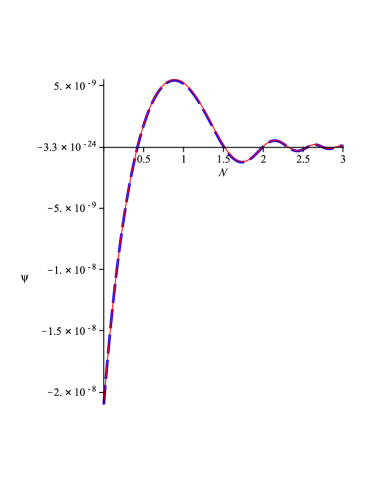
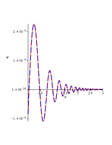
Figure 3: The evolution of the Bardeen potential $\Psi$ for sub-horizon modes with $k/H(0)=2$ and $10$ in the left and right panels respectively, for $f_{\rm d}=0.16$ and $\Gamma/H_{0}=10^{-8}$. In both plots, the thick dashed blue curve is the full numerical result while the thin solid red curve is the numerical solution obtained from Eq. (61).

V Primordial Black Hole Formation

Primordial black holes (PBHs) are a powerful tool for constraining models of the early Universe. Due to their gravitational effects and the consequences of their evaporation there are tight constraints on the number of PBHs that form (see e.g. Refs. Josan:2009qn ; Carr:2009jm ). These abundance constraints can be used to constrain the primordial power spectrum, and hence models of the early Universe, on scales far smaller than those probed by cosmological observations. We found in Sec. IV that the power spectrum is enhanced during the radiation dominated period after curvaton decay. In this section we therefore investigate whether this enhancement is sufficiently large to lead to PBH over production.

A region will collapse to form a PBH, with mass of order the horizon mass at that epoch, if the smoothed density contrast, in the comoving gauge, at horizon crossing ($R=c_{\rm s}(aH)^{-1}$ where $c_{\rm s}=1/\sqrt{3}$ is the sound speed), $\delta_{\rm com}(R=1/aH)\equiv\delta_{\rm hor}(R)$, satisfies the condition $\delta_{\rm hor}(R)\geq\delta_{\rm c}$ Carr:1985wss , where $\delta_{\rm c}\sim 1/3$ . The fraction of the energy density of the Universe contained in regions dense enough to form PBHs is then given, as in Press-Schechter theory Press:1973iz , by

$$\beta=2\frac{M_{\rm PBH}}{M_{H}}\int_{\delta_{\rm c}}^{\infty}P(\delta_{\rm hor}(R))\,{\rm d}\delta_{\rm hor}(R)\,.$$ (62)

Assuming that the initial primordial perturbations are Gaussian, the probability distribution of the smoothed density contrast, $P(\delta_{\rm hor}(R))$, is given by (e.g. Ref. LL )

$$P(\delta_{\rm hor}(R))=\frac{1}{\sqrt{2\pi}\sigma_{\rm hor}(R)}\exp{\left(-\frac{\delta_{\rm hor}^{2}(R)}{2\sigma_{\rm hor}^{2}(R)}\right)}\,,$$ (63)

where $\sigma(R)$ is the mass variance

$$\sigma^{2}(R)=\int_{0}^{\infty}W^{2}(kR)\mathcal{P}_{\delta}(k,t)\frac{\,{\rm d}k}{k}.$$ (64)

Here $W(kR)$ is the Fourier transform of the window function used to smooth the density contrast, which we take to be Gaussian, so that $W(kR)=\exp (-k^2{R}^2/2)$

References

- (1) D. H. Lyth and A. R. Liddle, “The primordial density perturbation”, Cambridge University Press (2009).
- (2) D. H. Lyth and D. Wands, “Generating the curvature perturbation without an inflaton,” Phys. Lett. B 524, 5 (2002) [arXiv:hep-ph/0110002].
- (3) K. Enqvist and M. S. Sloth, “Adiabatic CMB perturbations in pre - big bang string cosmology,” Nucl. Phys. B 626, 395 (2002) [hep-ph/0109214].
- (4) T. Moroi and T. Takahashi, “Effects of cosmological moduli fields on cosmic microwave background,” Phys. Lett. B 522, 215 (2001) [Erratum-ibid. B 539, 303 (2002)] [hep-ph/0110096].
- (5) N. Bartolo and A. R. Liddle, “The Simplest curvaton model,” Phys. Rev. D 65, 121301 (2002) [arXiv:astro-ph/0203076].
- (6) D. H. Lyth, C. Ungarelli and D. Wands, “The Primordial density perturbation in the curvaton scenario,” Phys. Rev. D 67, 023503 (2003) [arXiv:astro-ph/0208055].
- (7) D. H. Lyth and D. Wands, “The CDM isocurvature perturbation in the curvaton scenario,” Phys. Rev. D 68, 103516 (2003) [arXiv:astro-ph/0306500].
- (8) K. Dimopoulos, G. Lazarides, D. Lyth and R. Ruiz de Austri, “Curvaton dynamics,” Phys. Rev. D 68, 123515 (2003) [arXiv:hep-ph/0308015].
- (9) N. Bartolo, S. Matarrese and A. Riotto, “On nonGaussianity in the curvaton scenario,” Phys. Rev. D 69, 043503 (2004) [hep-ph/0309033].
- (10) K. A. Malik and D. H. Lyth, “A numerical study of non-gaussianity in the curvaton scenario,” JCAP 0609, 008 (2006) [astro-ph/0604387].
- (11) M. Sasaki, J. Valiviita and D. Wands, “Non-Gaussianity of the primordial perturbation in the curvaton model,” Phys. Rev. D 74, 103003 (2006) [astro-ph/0607627].
- (12) H. Assadullahi, J. Valiviita and D. Wands, “Primordial non-Gaussianity from two curvaton decays,” Phys. Rev. D 76, 103003 (2007) [arXiv:0708.0223 [hep-ph]].
- (13) K. Enqvist, S. Nurmi and G. I. Rigopoulos, “Parametric Decay of the Curvaton,” JCAP 0810, 013 (2008) [arXiv:0807.0382 [astro-ph]].
- (14) K. Dimopoulos, K. Kohri and T. Matsuda, “The hybrid curvaton,” Phys. Rev. D 85, 123541 (2012) [arXiv:1201.6037 [hep-ph]].
- (15) H. Assadullahi, H. Firouzjahi, M. H. Namjoo and D. Wands, “Curvaton and the inhomogeneous end of inflation,” arXiv:1207.7006 [astro-ph.CO].
- (16) K. A. Malik, D. Wands and C. Ungarelli, “Large scale curvature and entropy perturbations for multiple interacting fluids,” Phys. Rev. D 67 (2003) 063516 [arXiv:astro-ph/0211602].
- (17) S. Gupta, K. A. Malik and D. Wands, “Curvature and isocurvature perturbations in a three-fluid model of curvaton decay,” Phys. Rev. D 69, 063513 (2004) [arXiv:astro-ph/0311562].
- (18) V. F. Mukhanov, H. A. Feldman and R. H. Brandenberger, “Theory of cosmological perturbations. Part 1. Classical perturbations. Part 2. Quantum theory of perturbations. Part 3. Extensions,” Phys. Rept. 215, 203 (1992).
- (19) K. A. Malik and D. Wands, “Adiabatic and entropy perturbations with interacting fluids and fields,” JCAP 0502, 007 (2005) [astro-ph/0411703].
- (20) K. A. Malik and D. Wands, “Cosmological perturbations,” Phys. Rept. 475, 1 (2009) [arXiv:0809.4944 [astro-ph]].
- (21) D. Wands, K. A. Malik, D. H. Lyth and A. R. Liddle, “A New approach to the evolution of cosmological perturbations on large scales,” Phys. Rev. D 62, 043527 (2000) [astro-ph/0003278].
- (22) D. H. Lyth, K. A. Malik, M. Sasaki and I. Zaballa, “Forming sub-horizon black holes at the end of inflation,” JCAP 0601, 011 (2006) [arXiv:astro-ph/0510647].
- (23) I. Zaballa, A. M. Green, K. A. Malik and M. Sasaki, “Constraints on the primordial curvature perturbation from primordial black holes,” JCAP 0703, 010 (2007) [arXiv:astro-ph/0612379].
- (24) A. S. Josan, A. M. Green and K. A. Malik, “Generalised constraints on the curvature perturbation from primordial black holes,” Phys. Rev. D 79, 103520 (2009) [arXiv:0903.3184 [astro-ph.CO]].
- (25) B. J. Carr, K. Kohri, Y. Sendouda and J. Yokoyama,“New cosmological constraints on primordial black holes,” Phys. Rev. D 81 (2010) 104019 [arXiv:0912.5297 [astro-ph.CO]].
- (26) B. Carr, edited by J.L Sanz and L. Goicoechea, eds., in “Observational and theoretical aspects of relativistic astrophysics and cosmology”, World Scientific Singapore, 1985.
- (27) M. Kopp, S. Hofmann and J. Weller, “Separate Universes Do Not Constrain Primordial Black Hole Formation,” Phys. Rev. D 83 (2011) 124025 [arXiv:1012.4369 [astro-ph.CO]].
- (28) W. H. Press and P. Schechter, “Formation of Galaxies and Clusters of Galaxies by Self-Similar Gravitational Condensation,” Astrophys. J. 187 (1974) 425–438.