$NVU$ dynamics. III. Simulating molecules at constant potential energy

Abstract

This is the final paper in a series that introduces geodesic molecular dynamics at constant potential energy. This dynamics is entitled NVU dynamics in analogy to standard energy-conserving Newtonian NVE dynamics. In the first two papers [Ingebrigtsen et al., J. Chem. Phys. 135, 104101 (2011); ibid, 104102 (2011)], a numerical algorithm for simulating geodesic motion of atomic systems was developed and tested against standard algorithms. The conclusion was that the NVU algorithm has the same desirable properties as the Verlet algorithm for Newtonian NVE dynamics, i.e., it is time-reversible and symplectic. Additionally, it was concluded that NVU dynamics becomes equivalent to NVE dynamics in the thermodynamic limit. In this paper, the NVU algorithm for atomic systems is extended to be able to simulate geodesic motion of molecules at constant potential energy. We derive an algorithm for simulating rigid bonds and test this algorithm on three different systems: an asymmetric dumbbell model, Lewis-Wahnström OTP, and rigid SPC/E water. The rigid bonds introduce additional constraints beyond that of constant potential energy for atomic systems. The rigid-bond NVU algorithm conserves potential energy, bond lengths, and step length for indefinitely long runs. The quantities probed in simulations give results identical to those of Nosé-Hoover NVT dynamics. Since Nosé-Hoover NVT dynamics is known to give results equivalent to those of NVE dynamics, the latter results show that NVU dynamics becomes equivalent to NVE dynamics in the thermodynamic limit also for molecular systems.

I Introduction

In two recent papers^{1; 2} (henceforth: Papers I and II) molecular dynamics at constant potential energy was introduced, tested, and compared to well-known molecular dynamics algorithms. This new molecular dynamics is entitled NVU dynamics in analogy to standard energy-conserving Newtonian NVE dynamics. The conclusion was that NVU dynamics is a fully valid molecular dynamics, which for sufficiently large systems can be used interchangeably with NVE dynamics for calculating most quantities of interest. NVU dynamics is not faster than standard NVE or NVT dynamics, but introduces a new way of thinking about molecular dynamics. Molecular dynamics at constant potential energy was previously considered by Cotterill and co-workers^{3; 4; 5; 6}, by Scala et al.⁷, and most recently by Stratt and co-workers^{8; 9; 10; 11}, who actually allowed also lower potential energy values. Our motivation for studying NVU dynamics derived from recent work on strongly correlating liquids and their isomorphs^{12; 13; 14; 15; 16; 17; 18; 19} (see the Introduction of Paper I).

NVU dynamics is defined by geodesic motion on the constant-potential-energy hypersurface $\Omega$ defined by

$$\Omega=\{\textbf{R}\in R^{3N}\,\ |\,\ U(\textbf{R})=U_{0}\}.$$ (1)

Here $\textbf{R}\equiv\{\textbf{r}^{(1)},...,\textbf{r}^{(N)}\}$ in which $\textbf{r}^{(k)}$ is the position vector of the $k$’te particle (we follow here the notation of the Appendix of Paper II), and $U$ is the potential-energy function of an $N$-particle classical system. A geodesic on $\Omega$ is a curve that satisfies the condition of stationary length for fixed endpoints $\textbf{R}_{A}$ and $\textbf{R}_{B}$, i.e.,

$$\delta\int_{\textbf{R}_{A}}^{\textbf{R}_{B}}dl\,\ \Bigg{|}_{\Omega}=0,$$ (2)

where $dl$ is the line element of the metric. The shortest path between any two points is a geodesic. On a sphere geodesics are great circles, the ”straightest lines” of the surface. Traversing a geodesic at constant velocity thus corresponds to a generalization of Newton’s first law to a curved space (the surface itself).

In Paper I the NVU algorithm was developed via a discretization of Eq. (2), subsequently carrying out the variation. This technique, which is known as variational integration^{20; 21; 22; 23}, resulted in a ”basic” NVU algorithm that is similar to the well-known Verlet algorithm ${\bf R}_{i+1}\,=\,2{\bf R}_{i}-{\bf R}_{i-1}+(\Delta t)^{2}{\bf F}_{i}/m$ for Newtonian (NVE) dynamics ($m$ is the particle mass which is assumed identical in this section, and $\textbf{F}_{i}\equiv-\nabla_{\textbf{R}_{i}}U$ is the $3N$-dimensional force vector); the index $i$ refers to step $i$ of the integration sequence. In the Verlet algorithm $\Delta t$ is a fixed time step length. In comparison, the basic NVU algorithm is given by (Paper I)

$${\bf R}_{i+1}\,=\,2{\bf R}_{i}-{\bf R}_{i-1}+\frac{-2{\bf F}_{i}\cdot({\bf R}_{i}-{\bf R}_{i-1})}{{\bf F}_{i}^{2}}\,{\bf F}_{i}.$$ (3)

If the number of particles $N$ increases, the relative variation of the term $-2{\bf F}_{i}\cdot({\bf R}_{i}-{\bf R}_{i-1})/{\bf F}_{i}^{2}$ decreases, and this is why equivalence with Newtonian NVE dynamics is established in the thermodynamic limit. This equivalence should be understood in the sense that the relative deviations between, for instance, NVE and NVU auto-correlation functions go to zero as $N\to\infty$.

Paper I additionally developed a ”stabilized” version of the basic NVU algorithm to prevent accumulation of numerical errors. This version of the algorithm is given by (defining the position changes $\boldsymbol{\Delta}_{i+1/2}\equiv\textbf{R}_{i+1}-\textbf{R}_{i}$)

$$\boldsymbol{\Delta}_{i+1/2} =l_{0}\frac{\textbf{A}_{i-1/2}}{||\textbf{A}_{i-1/2}||},$$ (4)

$${\bf R}_{i+1} =\textbf{R}_{i}+\boldsymbol{\Delta}_{i+1/2},$$ (5)

where $l_{0}$ is the step length and

$$\textbf{A}_{i-1/2}=\frac{\boldsymbol{\Delta}_{i-1/2}+(-2{\bf F}_{i}\cdot\boldsymbol{\Delta}_{i-1/2}+U_{i-1}-U_{0})}{{\bf F}_{i}^{2}}\,{\bf F}_{i}.$$ (6)

All simulations in Papers I and II were performed with the stabilized algorithm. The basic algorithm was used, however, for theoretical considerations.

In this article we extend the stabilized NVU algorithm to deal with simulations of molecular systems. Molecular systems are simulated by introducing rigid and/or flexible bonds between the atoms in the modelling. Flexible bonds introduce merely an additional contribution to $U$, for instance, harmonic spring potentials. The basic NVU algorithm conserves the total potential energy and can readily simulate flexible bonds. The focus in this paper is thus on implementing rigid bonds in the framework of NVU dynamics.

Section II considers NVU dynamics with rigid bonds. Introducing rigid bonds in the simulations leads to Lagrangian multipliers in addition to those introduced in order to keep the potential energy constant (Paper I). Section II is fairly technical and easiest to read after reading Paper I. Section III gives simulation and model details. Section IV tests the rigid-bond NVU algorithm, and Sec. V investigates the NVU sampling properties by comparing the NVU results to Nosé-Hoover NVT results^{24; 25} on three different systems: the asymmetric dumbbell model²⁶, Lewis-Wahnström OTP²⁷, and rigid SPC/E water²⁸. Nosé-Hoover NVT dynamics is known to give results equivalent to NVE dynamics in the thermodynamic limit²⁹, and we refer to these dynamics interchangeably in the forthcoming sections. Finally, Sec. VI concludes.

II Rigid-bond $NVU$ algorithm

The rigid bonds^{30; 31} introduce constraints among the particle coordinates of the system. Each constraint $\alpha=1,...,G$ is of the form

$$\sigma_{\alpha}(\textbf{R})\equiv(\textbf{r}^{(k_{\alpha})}-\textbf{r}^{(l_{\alpha})})^{2}\equiv(\textbf{r}^{\alpha})^{2}=C_{\alpha}^{2};$$ (7)

it expresses that the distance between particles $k_{\alpha}$ and $l_{\alpha}$ is a constant, $C_{\alpha}$. In Papers I and II the integral of Eq. (2) was merely restricted to the constant-potential-energy hypersurface $\Omega$. Each rigid bond constraint introduces a function $\sigma_{\alpha}$ to be kept constant, and thus the integral of Eq. (2) is now further restricted to the sub-manifold $\omega$ of $\Omega$ where the bond constraints are satisfied,

$$\omega=\{\textbf{R}\in\Omega\,\ |\,\ \sigma_{\alpha}(\textbf{R})=C_{\alpha}\,\ ,\,\ \alpha=1,...,G\}.$$ (8)

If the bond constraints are independent, as assumed throughout the paper, $\omega$ is a (3N - G - 1)-dimensional compact Riemannian manifold. The variational principle defining NVU dynamics with rigid bonds is given by

$$\delta\int_{\textbf{R}_{A}}^{\textbf{R}_{B}}dl=0\,\ \Bigg{|}_{\omega}.$$ (9)

Most of Papers I and II dealt with the case of identical particle masses, but we wish here to develop a completely general molecular NVU algorithm. The line element $dl$ is defined by

$$dl^{2}\equiv\sum_{k}\tilde{m}_{k}\big{(}d{\bf r}^{(k)}\big{)}^{2},$$ (10)

where $\tilde{m}_{k}$ = $m_{k}/\langle m\rangle$ is the ”reduced” mass of particle $k$. Equation (10) is not the standard Euclidean line element, but a mass-weighted line element that goes back to Hertz^{32; 33}. We shall refer to this metric as the ”Hertzian” metric. The point of this particular metric is that it ensures equivalence between NVU and NVE dynamics for systems of atoms and molecules of varying mass. In appendix A we derive the variable-mass atomic NVU algorithm applying the Hertzian metric (correcting also a typo of the Appendix of Paper II).

Applying the variational integration technique to Eq. (9) gives

$$\delta\left(\sum_{i}\sqrt{\sum_{k}\tilde{m}_{k}\left(\textbf{r}_{i}^{(k)}-\textbf{r}_{i-1}^{(k)}\right)^{2}}-\sum_{i}\lambda_{i}U({\bf R}_{i})+\sum_{i,\alpha}\Lambda_{\alpha i}\sigma_{\alpha}(\textbf{R}_{i})\right)\,=\,0\,.$$ (11)

In Eq. (11) the path is divided into a number of discrete points and one Lagrangian multiplier $\Lambda_{\alpha i}$ is introduced for each constraint $\alpha$ at every point $i$. Following standard notation for constraint molecular dynamics^{31; 30}, the Lagrangian multipliers of the bond constraints are chosen with a positive sign. As in Papers I and II we now make the Ansatz of constant step length $l_{0}$, i.e.,

$$\sum_{k}\tilde{m}_{k}\left(\textbf{r}_{i}^{(k)}-\textbf{r}_{i-1}^{(k)}\right)^{2}\equiv l_{0}^{2}.$$ (12)

Carrying out the variation of Eq. (11) using Eq. (12) leads to (compare the derivation in Paper I)

$$\textbf{r}_{i+1}^{(k)}=2\textbf{r}_{i}^{(k)}-\textbf{r}_{i-1}^{(k)}+\frac{l_{0}}{\tilde{m}_{k}}\lambda_{i}\textbf{f}_{i}^{(k)}+\frac{l_{0}}{\tilde{m}_{k}}\nabla_{\textbf{r}_{i}^{(k)}}\sum_{\alpha}\Lambda_{\alpha i}\sigma_{\alpha},$$ (13)

where $\textbf{f}_{i}^{(k)}=-\nabla_{\textbf{r}_{i}^{(k)}}U$ is the force on particle $k$ at step $i$. This equation constitutes the NVU algorithm with rigid bonds. It has a close resemblance to the Lagrangian equations of motion with holonomic constraints³¹, i.e., rigid-bond NVE dynamics³⁰. Equation (13) contains $G+1$ Lagrangian multipliers for each integration step, which must be determined to complete the algorithm.

II.1 Determining the NVU Lagrangian multipliers

This section shows how to calculate the Lagrangian multipliers. Since the algorithm is to be implemented on a computer (with finite-precision), we shall proceed directly to a ”stabilized” algorithm conserving for indefinitely long runs potential energy, bond lengths, and step length (in $3N$-dimensions). The resulting algorithm reduces to the stabilized atomic NVU algorithm of Eqs. (4)-(6) in the case of no bonds constraints.

Some notation used in the following derivation is now introduced (the nomenclature of text is summarized in Table 1).

Symbol	Definition
$\sigma_{\alpha}(\textbf{R})$	The $\alpha$’te bond constraint between particles $k_{\alpha}$ and $l_{\alpha}$ with $\alpha=1,...,G$. ($\sigma_{\alpha}=(\textbf{r}^{\alpha})^{2}=C_{\alpha}^{2}$).
$\tilde{m}_{k}$	The mass of particle $k$ divided by the average mass of the system. ($\tilde{m}_{k}=m_{k}/\langle m\rangle$).
	3-dimensional vectors
$\textbf{r}^{(k)}_{i}$	Position of particle $k$ at step $i$.
$\boldsymbol{\delta}_{i+1/2}^{(k)}$	Displacement of the position of particle $k$ between step $i$ and $i+1$. ($\boldsymbol{\delta}_{i+1/2}^{(k)}=\textbf{r}_{i+1}^{(k)}-\textbf{r}_{i}^{(k)}$).
$\textbf{f}^{(k)}_{i}$	Force on particle $k$ at step $i$. ($\textbf{f}^{(k)}_{i}=-\nabla_{\textbf{r}^{(k)}_{i}}U$).
$\textbf{g}^{(k)}_{i}$	Constraint force on particle $k$ at step $i$. ($\textbf{g}_{i}^{(k)}=\nabla_{\textbf{r}_{i}^{(k)}}\sum_{\alpha}\Lambda_{\alpha i}\sigma_{\alpha}$).
$\textbf{r}_{i}^{\alpha}$	Displacement of the positions of particles $k_{\alpha}$ and $l_{\alpha}$ at step $i$. ($\textbf{r}_{i}^{\alpha}=\textbf{r}_{i}^{(k_{\alpha})}-\textbf{r}_{i}^{(l_{\alpha})}$).
$\boldsymbol{\delta}_{i-1/2}^{\alpha}$	Displacement of the velocities of particles $k_{\alpha}$ and $l_{\alpha}$ at step $i-1/2$. ($\boldsymbol{\delta}_{i-1/2}^{\alpha}=\boldsymbol{\delta}^{(k_{\alpha})}_{i-1/2}-\boldsymbol{\delta}^{(l_{\alpha})}_{i-1/2}$).
$\textbf{s}_{i}^{\alpha}$	Sum of displacements of positions and velocities of particles $k_{\alpha}$ and $l_{\alpha}$ at, respectively, step $i$ and $i-1/2$. $(\textbf{s}_{i}^{\alpha}=\textbf{r}_{i}^{\alpha}+\boldsymbol{\delta}_{i-1/2}^{\alpha}$).
$\tilde{\textbf{f}}^{\alpha}_{i}$	Displacement of the forces on particles $k_{\alpha}$ and $l_{\alpha}$ at step $i$ divided by their reduced particle mass. ($\tilde{\textbf{f}}_{i}^{\alpha}=\textbf{f}_{i}^{(k_{\alpha})}/\tilde{m}_{k_{\alpha}}-{\textbf{f}}_{i}^{(l_{\alpha})}/\tilde{m}_{l_{\alpha}}$).
$\tilde{\textbf{g}}^{\alpha}_{i}$	Displacement of the constraint forces on particles $k_{\alpha}$ and $l_{\alpha}$ at step $i$ divided by their reduced particle mass. ($\tilde{\boldsymbol{g}}^{\alpha}_{i}=\textbf{g}_{i}^{(k_{\alpha})}/\tilde{m}_{k_{\alpha}}-{\textbf{g}}_{i}^{(l_{\alpha})}/\tilde{m}_{l_{\alpha}}$).
	$3N$-dimensional vectors
$\textbf{R}_{i}$	Position of all particles at step $i$. ($\textbf{R}_{i}=\{\textbf{r}_{i}^{(1)},...,\textbf{r}_{i}^{(N)}\}$).
$\boldsymbol{\Delta}_{i+1/2}$	Displacement of the positions between step $i$ and $i+1$. ($\boldsymbol{\Delta}_{i+1/2}=\textbf{R}_{i+1}-\textbf{R}_{i}$).
$\textbf{F}_{i}$	Force on all particles at step $i$. ($\textbf{F}_{i}=-\nabla_{\textbf{R}_{i}}U$).
$\tilde{\textbf{F}}_{i}$	Force on all particles at step $i$ divided by the reduced particle mass. ($\tilde{\textbf{F}}_{i}=\{\textbf{f}_{i}^{(1)}/\tilde{m}_{1},...,\textbf{f}_{i}^{(N)}/\tilde{m}_{N}\}$).
$\tilde{\textbf{G}}_{i}$	Constraint force on all particles at step $i$ divided by the reduced particle mass. ($\tilde{\textbf{G}}_{i}=\{\textbf{g}_{i}^{(1)}/\tilde{m}_{1},...,\textbf{g}_{i}^{(N)}/\tilde{m}_{N}\}$).

Table 1: Definitions and nomenclature of the text.

Defining $\boldsymbol{\delta}_{i+1/2}^{(k)}\equiv\textbf{r}_{i+1}^{(k)}-\textbf{r}_{i}^{(k)}$ and $\textbf{g}_{i}^{(k)}\equiv\nabla_{\textbf{r}_{i}^{(k)}}\sum_{\alpha}\Lambda_{\alpha i}\sigma_{\alpha}$ the ”Leap-frog”³⁴ version of the rigid-bond NVU algorithm Eq. (13) reads

$$\boldsymbol{\delta}_{i+1/2}^{(k)} =\boldsymbol{\delta}_{i-1/2}^{(k)}+\frac{l_{0}}{\tilde{m}_{k}}\lambda_{i}\textbf{f}_{i}^{(k)}+\frac{l_{0}}{\tilde{m}_{k}}\textbf{g}_{i}^{(k)},$$ (14)

$$\textbf{r}_{i+1}^{(k)} =\textbf{r}_{i}^{(k)}+\boldsymbol{\delta}_{i+1/2}^{(k)}.$$ (15)

In analogy to rigid-bond NVE dynamics we call $\textbf{g}^{(k)}_{i}$ the ”constraint force” on particle $k$ at step $i$. Introducing the notation $\tilde{\textbf{F}}_{i}\equiv\{\textbf{f}_{i}^{(1)}/\tilde{m}_{1},...,\textbf{f}_{i}^{(N)}/\tilde{m}_{N}\}$ and $\tilde{\textbf{G}}_{i}\equiv\{\textbf{g}^{(1)}_{i}/\tilde{m}_{1},...,\textbf{g}^{(N)}_{i}/\tilde{m}_{N}\}$, the NVU algorithm in the full $3N$-dimensional coordinate space reads

$$\boldsymbol{\Delta}_{i+1/2} =\boldsymbol{\Delta}_{i-1/2}+l_{0}\lambda_{i}\tilde{\textbf{F}}_{i}+l_{0}\tilde{\textbf{G}}_{i},$$ (16)

$$\textbf{R}_{i+1} =\textbf{R}_{i}+\boldsymbol{\Delta}_{i+1/2},.$$ (17)

The Lagrangian multipliers are calculated by combining a result derived in Paper I with the method applied in the SHAKE algorithm³⁰ for rigid bonds in NVE dynamics^{30; 35; 36}. The SHAKE algorithm calculates the Lagrangian multipliers from the equations $(\textbf{r}_{i+1}^{\alpha})^{2}=C^{2}_{\alpha}$. In doing so, the target value of the constraints $C_{\alpha}$ appears explicitly in the algorithm, making the bond lengths insensitive to numerical error. The expression for $\textbf{r}_{i+1}^{\alpha}$ is supplied by the integration algorithm containing herein the Lagrangian multipliers. In our case, this gives $G$ equations with $G+1$ unknowns. The missing equation is supplied by an expression derived in Paper I, namely that $U_{i+1}$ = $U_{i-1}-\textbf{F}_{i}\cdot(\textbf{R}_{i+1}-\textbf{R}_{i-1})$ to third order in the step length. In the discrete sequence of points $U_{i+1}$ is set equal to $U_{0}$ (the constant defining $\Omega$), making the constraint of constant potential energy also insensitive to numerical error. We thus have the following $G+1$ equations for calculating the Lagrangian multipliers

$$U_{i-1}-\textbf{F}_{i}\cdot(\textbf{R}_{i+1}-\textbf{R}_{i-1})-U_{0} =0,$$ (18)

$$(\textbf{r}_{i+1}^{\alpha})^{2}-C^{2}_{\alpha} =0,\,\ (\alpha=1,...,G).$$ (19)

By Eqs. (16) and (17); $\textbf{R}_{i+1}-\textbf{R}_{i-1}$ = $\boldsymbol{\Delta}_{i+1/2}+\boldsymbol{\Delta}_{i-1/2}$ = $2\boldsymbol{\Delta}_{i-1/2}+l_{0}\lambda_{i}\tilde{\textbf{F}}_{i}+l_{0}\tilde{\textbf{G}}_{i}$. Defining $\boldsymbol{\delta}^{\alpha}_{i-1/2}\equiv\boldsymbol{\delta}^{(k_{\alpha})}_{i-1/2}-\boldsymbol{\delta}^{(l_{\alpha})}_{i-1/2}$, $\tilde{\textbf{f}}_{i}^{\alpha}\equiv\textbf{f}_{i}^{(k_{\alpha})}/\tilde{m}_{k_{\alpha}}-{\textbf{f}}_{i}^{(l_{\alpha})}/\tilde{m}_{l_{\alpha}}$, and $\tilde{\boldsymbol{g}}^{\alpha}_{i}\equiv\textbf{g}_{i}^{(k_{\alpha})}/\tilde{m}_{k_{\alpha}}-{\textbf{g}}_{i}^{(l_{\alpha})}/\tilde{m}_{l_{\alpha}}$, since by Eqs. (14) and (15); $\textbf{r}^{\alpha}_{i+1}$ = $\textbf{r}^{(k_{\alpha})}_{i+1}-\textbf{r}^{(l_{\alpha})}_{i+1}$ = $\textbf{r}_{i}^{(k_{\alpha})}-\textbf{r}_{i}^{(l_{\alpha})}+\boldsymbol{\delta}_{i+1/2}^{(k_{\alpha})}-\boldsymbol{\delta}_{i+1/2}^{(l_{\alpha})}$ = $\textbf{r}^{\alpha}_{i}+\boldsymbol{\delta}^{\alpha}_{i-1/2}+l_{0}\lambda_{i}\tilde{\textbf{f}}_{i}^{\alpha}+l_{0}\tilde{\textbf{g}}_{i}^{\alpha}$, it follows that

$$U_{i-1}-\textbf{F}_{i}\cdot\Big{[}2\boldsymbol{\Delta}_{i-1/2}+l_{0}\lambda_{i}\tilde{\textbf{F}}_{i}+l_{0}\tilde{\textbf{G}}_{i}\Big{]}-U_{0} =0,$$ (20)

$$\Big{[}\textbf{r}^{\alpha}_{i}+\boldsymbol{\delta}^{\alpha}_{i-1/2}+l_{0}\lambda_{i}\tilde{\textbf{f}}_{i}^{\alpha}+l_{0}\tilde{\textbf{g}}_{i}^{\alpha}\Big{]}^{2}-C^{2}_{\alpha} =0,\,\ (\alpha=1,...,G).$$ (21)

The above coupled quadratic equations for the Lagrangian multipliers are now solved following the produce of the MILC-SHAKE algorithm³⁷, which starts by neglecting the second order terms in the Lagrangian multipliers and solving the resulting linear equations. Afterwards, the second order terms are taken into account in an iterative manner - the details of which are described below.

For each integration step $i$, the linearized equations are given by

$$\textbf{A}_{i}\boldsymbol{\lambda}_{i}=\textbf{b}_{i},$$ (22)

where $\textbf{A}_{i}$ is a $(G+1)\times(G+1)$ matrix, $\boldsymbol{\lambda}_{i}\equiv\{\lambda_{i},\Lambda_{1i},...,\Lambda_{Gi}\}$, and $\textbf{b}_{i}$ a $G+1$ column vector. We start by calculating explicitly the first few elements of the matrix $\textbf{A}_{i}$. $A_{11}$ consists merely of the factor infront of $\lambda_{i}$ in Eq. (20), i.e., $A_{11}=-l_{0}\tilde{\textbf{F}}_{i}\cdot\textbf{F}_{i}$. The second element $A_{12}$ appears after expansion of the dot product $\textbf{F}_{i}\cdot\tilde{\textbf{G}}_{i}$. Noting that $\nabla_{\textbf{r}_{i}^{(k_{\alpha})}}\sigma_{\alpha}=2\textbf{r}_{i}^{\alpha}$, we have $\textbf{F}_{i}\cdot\tilde{\textbf{G}}_{i}$ = $\textbf{f}_{i}^{(1)}\cdot\textbf{g}_{i}^{(1)}/\tilde{m}_{1}+...+\textbf{f}_{i}^{(N)}\cdot\textbf{g}_{i}^{(N)}/\tilde{m}_{N}$ = 2$\Lambda_{1i}(\tilde{\textbf{f}}^{1}_{i}\cdot\textbf{r}_{i}^{1})+...+2\Lambda_{Gi}(\tilde{\textbf{f}}^{G}_{i}\cdot\textbf{r}_{i}^{G})$. The last equation follows as the Lagrangian multipliers appear in pairs, differing only by the sign from $\nabla_{\textbf{r}_{i}^{(k_{\alpha})}}\sigma_{\alpha}$ and the term $\textbf{f}_{i}^{(k_{\alpha})}/\tilde{m}_{k_{\alpha}}$. We thus find $A_{12}$ = $-2l_{0}\tilde{\textbf{f}}^{1}_{i}\cdot\textbf{r}_{i}^{1}$, $A_{13}=-2l_{0}\tilde{\textbf{f}}^{2}_{i}\cdot\textbf{r}_{i}^{2}$, etc. In the second row of $\textbf{A}_{i}$, the short-hand notation $\textbf{s}^{\alpha}_{i}\equiv\textbf{r}_{i}^{\alpha}+\boldsymbol{\delta}^{\alpha}_{i-1/2}$ is introduced, making $A_{21}$ = $2l_{0}(\textbf{s}^{1}_{i}\cdot\tilde{\textbf{f}}^{1}_{i})$, i.e., the factor infront of $\lambda_{i}$ after squaring of the parentheses. The next element $A_{22}$ appears after expanding $\textbf{s}_{i}^{1}\cdot\tilde{\textbf{g}}^{1}_{i}$ = $\boldsymbol{s}^{1}_{i}\cdot\sum_{\beta}\Lambda_{\beta i}(\frac{1}{\tilde{m}_{k_{1}}}\nabla_{\textbf{r}_{i}^{(k_{1})}}\sigma_{\beta}-\frac{1}{\tilde{m}_{l_{1}}}\nabla_{\textbf{r}_{i}^{(l_{1})}}\sigma_{\beta})$. In this sum, we identify the factor in front of $\Lambda_{1i}$, giving $A_{22}$ = $2l_{0}\boldsymbol{s}^{1}_{i}\cdot(\frac{1}{\tilde{m}_{k_{1}}}\nabla_{\textbf{r}_{i}^{(k_{1})}}\sigma_{1}-\frac{1}{\tilde{m}_{l_{1}}}\nabla_{\textbf{r}_{i}^{(l_{1})}}\sigma_{1})$, and similarly for the remaining elements of the second row.

Altogether, the elements of $\textbf{A}_{i}$ are thus given by

$$\textbf{A}_{i} =2l_{0}\begin{pmatrix}-\tilde{\textbf{F}}_{i}\cdot\textbf{F}_{i}/2&-\tilde{\textbf{f}}_{i}^{1}\cdot\textbf{r}^{1}_{i}&\cdots&-\tilde{\textbf{f}}_{i}^{G}\cdot\textbf{r}^{G}_{i}\\ \boldsymbol{s}^{1}_{i}\cdot\tilde{\textbf{f}}_{i}^{1}&\boldsymbol{s}^{1}_{i}\cdot(\frac{1}{\tilde{m}_{k_{1}}}\nabla_{\textbf{r}_{i}^{(k_{1})}}\sigma_{1}-\frac{1}{\tilde{m}_{l_{1}}}\nabla_{\textbf{r}_{i}^{(l_{1})}}\sigma_{1})&\cdots&\boldsymbol{s}^{1}_{i}\cdot(\frac{1}{\tilde{m}_{k_{1}}}\nabla_{\textbf{r}_{i}^{(k_{1})}}\sigma_{G}-\frac{1}{\tilde{m}_{l_{1}}}\nabla_{\textbf{r}_{i}^{(l_{1})}}\sigma_{G})\\ \vdots&\vdots&\vdots&\vdots\\ \boldsymbol{s}^{G}_{i}\cdot\tilde{\textbf{f}}_{i}^{G}&\boldsymbol{s}^{G}_{i}\cdot(\frac{1}{\tilde{m}_{k_{G}}}\nabla_{\textbf{r}_{i}^{(k_{G})}}\sigma_{1}-\frac{1}{\tilde{m}_{l_{G}}}\nabla_{\textbf{r}_{i}^{(l_{G})}}\sigma_{1})&\cdots&\boldsymbol{s}^{G}_{i}\cdot(\frac{1}{\tilde{m}_{k_{G}}}\nabla_{\textbf{r}_{i}^{(k_{G})}}\sigma_{G}-\frac{1}{\tilde{m}_{l_{G}}}\nabla_{\textbf{r}_{i}^{(l_{G})}}\sigma_{G})\end{pmatrix}.$$ (23)

The column vector $\textbf{b}_{i}$ consists of all zeroth-order terms in Eqs. (20) and (21)

$$\textbf{b}_{i} =\begin{pmatrix}U_{0}-U_{i-1}+2\textbf{F}_{i}\cdot\boldsymbol{\Delta}_{i-1/2}\\ C^{2}_{1}-(\textbf{s}^{1}_{i})^{2}\\ \vdots\\ C^{2}_{G}-(\textbf{s}^{G}_{i})^{2}\end{pmatrix}.$$ (24)

Turning now to the iteration procedure, the second-order terms in the Lagrangian multipliers (Eq. (21)) are taken into account by iterating the right-hand side of Eq. (22) via the scheme ($\alpha=1,...,G$)

$$b_{\alpha}^{j+1}=b_{\alpha}^{j}+\Big{[}C_{\alpha}^{2}-\big{(}(\textbf{r}_{i+1}^{\alpha})^{2}\big{)}^{j}\Big{]}.$$ (25)

The superscript $j$ refers here to iteration $j$, and $\big{(}(\textbf{r}_{i+1}^{\alpha})^{2}\big{)}^{j}$ are the positions associated with iteration $j$. The element $b_{0}$ is not updated as it derives from the constraint of constant potential energy. For each iteration $j$ the term $C_{\alpha}^{2}-\big{(}(\textbf{r}_{i+1}^{\alpha})^{2}\big{)}^{j}$ is expected to become smaller as the bonds are satisfied better and better, and convergence was achieved within a few iterations³⁷.

For each integration step $i$, the algorithm for determining the NVU Lagrangian multipliers thus proceeds as follows

1. The Lagrangian multipliers of iteration $j$, $(\boldsymbol{\lambda}_{i})^{j}$, are calculated from Eq. (22).

2. $\big{(}(\textbf{r}_{i+1}^{\alpha})^{2}\big{)}^{j}$ is calculated via Eqs. (14) and (15) using $(\boldsymbol{\lambda}_{i})^{j}$.

3. $\textbf{b}_{i}$ is updated via Eq. (25) from $\big{(}(\textbf{r}_{i+1}^{\alpha})^{2}\big{)}^{j}$.

4. The above steps are repeated (starting iteration $j+1$) until convergence is established (we used a preset number of iterations, typically 3-5).

How is constant step length $l_{0}$ ensured numerically? Generalizing the approach of Paper I we introduce a normalizing factor such that

$$\boldsymbol{\delta}_{i+1/2}^{(k)} =l_{0}\frac{\boldsymbol{\chi}^{(k)}_{i-1/2}}{\sqrt{\sum_{k}\tilde{m}_{k}(\boldsymbol{\chi}_{i-1/2}^{(k)})^{2}}},$$ (26)

$$\textbf{r}_{i+1}^{(k)} =\textbf{r}_{i}^{(k)}+\boldsymbol{\delta}_{i+1/2}^{(k)},$$ (27)

where

$$\boldsymbol{\chi}_{i-1/2}^{(k)}\equiv\boldsymbol{\delta}_{i-1/2}^{(k)}+\frac{l_{0}}{\tilde{m}_{k}}\lambda_{i}\textbf{f}_{i}^{(k)}+\frac{l_{0}}{\tilde{m}_{k}}\textbf{g}_{i}^{(k)}.$$ (28)

The normalizing factor is close to unity¹ and ensures trivially $\sum_{k}\tilde{m}_{k}(\boldsymbol{\delta}_{i+1/2}^{(k)})^{2}$ = $l^{2}_{0}$, i.e., that the step length is conserved. The algorithm is now absolutely stable, conserving potential energy, bond lengths, and step length for indefinitely long runs. The stability of the NVU algorithm is tested numerically in Sec. IV.

II.2 Alternative determination of the NVU Lagrangian multipliers

The previous section followed the traditional way of calculating the Lagrangian multipliers. The NVU Lagrangian multipliers may also be calculated by Taylor expanding the constraints $\sigma_{\alpha}$ in analogy to the method sketched above for the potential energy. In this way, the constraints of constant potential energy and constant bond lengths are treated on equal footing. The set of equations to be solved is the following (recall that $\textbf{R}_{i+1}-\textbf{R}_{i-1}$ = $2\boldsymbol{\Delta}_{i-1/2}+l_{0}\lambda_{i}\tilde{\textbf{F}}_{i}+l_{0}\tilde{\textbf{G}}_{i}$)

$$U_{i-1}-\textbf{F}_{i}\cdot(\textbf{R}_{i+1}-\textbf{R}_{i-1})-U_{0} =0,$$ (29)

$$\sigma_{\alpha(i-1)}+\nabla_{\textbf{R}_{i}}\sigma_{\alpha i}\cdot(\textbf{R}_{i+1}-\textbf{R}_{i-1})-C^{2}_{\alpha} =0,\,\ (\alpha=1,...,G).$$ (30)

The determination of the Lagrangian multipliers is linear and thus no iterations are needed. The bond constraints $\sigma_{\alpha}$ are obeyed to the same order $O(l_{0}^{3})$ as the constraint of constant potential energy. The sampling properties of this novel, alternative determination method is tested briefly in Sec. V. It appears to be a promising new way of determining the Lagrangian multipliers in connection with rigid bonds, which might also be useful for standard bond-constraint NVE or NVT simulations.

III Simulation details and model systems

We investigated three systems: The asymmetric dumbbell model, the Lewis-Wahnström OTP model, and rigid SPC/E water. For all simulated pair potentials the shifted-force truncation scheme was applied at a cut-off radius $r_{c}$. If the pair potential is $v(r)$ and the pair force is $f(r)=-v^{\prime}(r)$, the shifted force is given by^{34; 38}

$$f_{\rm SF}(r)\,=\,\begin{cases}f(r)-f(r_{c})&\text{if}\,\,r<r_{c}\,,\\ 0&\text{if}\,\,r>r_{c}\,.\end{cases}$$ (31)

This corresponds to using the following pair potential below $r_{c}$: $v_{\rm SF}(r)=v(r)-v^{\prime}(r_{c})(r-r_{c})-v(r_{c})$. All simulations were performed with the NVT and NVU algorithms. Recall that NVE and NVT dynamics give equivalent results²⁹; for this reason no simulations are presented for NVE dynamics. The RUMD code³⁹ was used for molecular dynamics simulations (an optimized open-source GPU code). The NVT ensemble is generated via the Nosé-Hoover algorithm^{24; 25; 40}, and the bonds held fixed using the time-reversible constraint algorithm of Refs. ³⁵; ³⁶. The NVU algorithm is described in Sec. II. The starting files for NVU dynamics were taken from an equilibrated NVT simulation. The positions and velocities of the NVT configuration do not correspond perfectly to motion on $\omega$, since the potential energy and step length are not those of $U_{0}$ and $l_{0}$, respectively. As all three constraints are to be satisfied simultaneously, this results in numerical problems when starting the simulation from the particular NVT configuration. A more gentle procedure is thus applied, where the atomic NVU algorithm is used for a couple of integration steps to ensure the values of $U_{0}$ and $l_{0}$. Afterwards, the rigid-bond NVU algorithm is used.

III.1 NVU iteration procedure

The quadratic equations (Eq. (25)) were iterated with a fixed number of iterations (between 3 and 5). The linear systems were solved utilizing CUSP⁴¹, a library for solving systems of linear equations on the GPU. More specifically, the stabilized biconjugate gradient algorithm with a Jacobi preconditioner⁴² was used with the initial value $\boldsymbol{\lambda}_{i}=0$. The relative tolerance $\tau$ for the asymmetric dumbbell and Lewis-Wahnström OTP models was chosen as $\tau=10^{-7}$ and for rigid SPC/E water as $\tau=3\cdot 10^{-7}$. A larger tolerance was chosen for rigid SPC/E water due to convergence issues in connection with shifted-force Coulomb interactions (see below).

The maximum number of allowed iterations was 50. A restart scheme was applied when the solver did not converge within the chosen tolerance. In this case the solver (and quadratic iteration) was restarted from the partially estimated ”solution” adding $2\cdot 10^{-7}$ to the tolerance. It should be noted that the stabilized biconjugate gradient algorithm may get ”trapped”, resulting in a break-down of the CUSP linear solver. If this happens, it is detected by our program, and the solver and quadratic iteration are restarted, with a smaller number (10) of maximum allowed iterations for the solver.

III.2 The asymmetric dumbbell

The asymmetric dumbbell model²⁶ consists of a large ($A$) and a small ($B$) Lennard-Jones (LJ) particle, rigidly bonded with bond distance of $r_{AB}=0.29/0.4963$ (here and henceforth units are given in LJ units referring to the $A$ particle such that $\sigma_{AA}$ = 1, $\epsilon_{AA}$ = 1, and $m_{A}$ = 1). The asymmetric dumbbell model has $\sigma_{BB}=0.3910/0.4963$, $\epsilon_{BB}=0.66944/5.726$, and $m_{B}=15.035/77.106$. The $AB$ interaction between different molecules is determined by the Lorentz-Berthelot mixing rule³⁴. $n$ = 500 molecules (here and henceforth $n$ denotes the number of molecules and $N$ the number of atoms) were used in the simulations with a pair-potential cut-off of $r_{c}=2.5$. The step length $l_{0}$ was fixed in the range 0.125-0.138 depending on the state point.

Simulations were also performed where the rigid bonds were replaced with stiff harmonic springs. The spring constant was $k=3000$, while all other model parameters remained unchanged.

III.3 Lewis-Wahnström OTP

The Lewis-Wahnström OTP model²⁷ consists of three identical LJ particles rigidly bonded in an isosceles triangle with sides of $r_{AA}=1$ and top angle of $75^{\circ}$. All parameters (including the masses) are unity for the OTP model. $n$ = 320 molecules were simulated and a pair-potential cut-off of $r_{c}=2.5$ was used. The step length was 0.100.

III.4 SPC/E Water

The SPC/E water model²⁸ is an isosceles triangle with sides $r_{OH}=1/3.166$ and top angle $109.47^{\circ}$. The $OO$ intermolecular interactions are given by the LJ pair potential ($\epsilon_{OO}=1$, $\sigma_{OO}=1$, and $m_{O}=15.9994/1.00794$). The three particles are charged with $q_{O}=-22.0$ and $q_{H}=|q_{O}|/2$. $n$ = 2000 molecules were simulated and a pair-potential cut-off of $r_{c}=6.28$ for both LJ and Coulomb interactions was applied^{43; 44}. The step length was fixed in the range 0.06-0.07 depending on the state point. For this system the numerical stability is surprisingly sensitive to the cut-off used in the Coulomb interactions, but a larger shifted-force cut-off improves this behavior⁴⁴.

IV Testing the stability of the rigid-bond $NVU$ algorithm

This section tests the conservation properties of the rigid-bond NVU algorithm. Table 2 shows the potential energy, the deviation of bond lengths, and step length as functions of integration step number for Lewis-Wahnström OTP at $\rho$ = 0.329 and T = 0.700. It is clear that these quantities are conserved by the algorithm and that no drift occurs. The step length is conserved to the highest accuracy since it is not prone to numerical error in determining the Lagrangian multipliers.

Integration steps	$U$ / $N$	$(1/G\sum_{\alpha}(r^{\alpha}$ $-$ $C_{\alpha})^{2})^{1/2}$	$\sum_{k}\tilde{m}_{k}(\boldsymbol{\delta}_{i+1/2}^{(k)})^{2}$
$10^{1}$	-4.42550	2.81207 $\cdot 10^{-7}$	0.0999999
$10^{2}$	-4.42552	3.03535 $\cdot 10^{-7}$	0.1000000
$10^{3}$	-4.42552	2.81128 $\cdot 10^{-7}$	0.1000000
$10^{4}$	-4.42552	2.95078 $\cdot 10^{-7}$	0.1000000
$10^{5}$	-4.42550	3.08793 $\cdot 10^{-7}$	0.1000000
$10^{6}$	-4.42551	2.90477 $\cdot 10^{-7}$	0.1000000

Table 2: Potential energy, deviation of bond lengths and step length as functions of integration step number in the NVU algorithm for Lewis-Wahnström OTP ($\rho$ = 0.329, T = 0.700). Single-precision floating-point arithmetic was used for the simulations.

Figure 1 shows the distribution of the term $l_{0}\lambda_{i}\langle m\rangle$ in Eq. (13) (recall $\tilde{m}_{k}=m_{k}/\langle m\rangle$). In NVU dynamics there is, as such, no notation of time; a geodesic on the manifold can be traversed with any velocity. Comparing the NVU algorithm of Eq. (13) to the rigid-bond Verlet algorithm³⁰ ${\bf r}^{(k)}_{i+1}\,=\,2{\bf r}^{(k)}_{i}-{\bf r}^{(k)}_{i-1}+((\Delta t)^{2}/m_{k})[\textbf{f}^{(k)}_{i}+\textbf{g}^{(k)}_{i}]$, we can define the term $l_{0}\lambda_{i}\langle m\rangle$ as a varying ”time step” length of the NVU algorithm (see also Paper II), i.e.,

$$(\Delta t_{i,NVU})^{2}\equiv l_{0}\lambda_{i}\langle m\rangle.$$ (32)

The integration steps of the NVU algorithm are thus henceforth referred to as ”time steps”. The average of Eq. (32) is used in Sec. V when comparing to NVT dynamics. As was the case for the atomic NVU algorithm (Paper I), $l_{0}\lambda_{i}\langle m\rangle$ is Gaussian distributed for large systems and its relative variation decreases as the number of particles increases. It thus becomes a better and better approximation to treat this term as constant, implying equivalent sampling properties of NVU and NVE dynamics also when rigid bonds are included in the simulations.

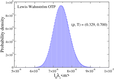
Figure 1: The probability density of the ”time step” length $(\Delta t_{i,NVU})^{2}\equiv l_{0}\lambda_{i}\langle m\rangle$ of the rigid-bond NVU algorithm for Lewis-Wahnström OTP at $\rho$ = 0.329 and T = 0.700. $n=320$ molecules were used in the simulations.

V Sampling properties of the rigid-bond $NVU$ algorithm

The NVU algorithm is now compared to NVT dynamics for the three different models. First, we consider the asymmetric dumbbell model²⁶, both rigid and flexible. Afterwards, the Lewis-Wahnström OTP model²⁷, and finally rigid SPC/E water²⁸.

V.1 The asymmetric dumbbell model

In Figs. 2(a) and (b) are shown, respectively, the molecular center-of-mass (CM) radial distribution functions and the CM incoherent intermediate scattering functions for the rigid asymmetric dumbbell model²⁶ for different temperatures at $\rho=0.932$. The black circles and curves give NVT simulation results while the red crosses give the NVU simulation results. The two radial distribution functions in Fig. 2(a) agree very well, and this is also the case for the dynamics in Fig. 2(b).

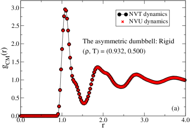
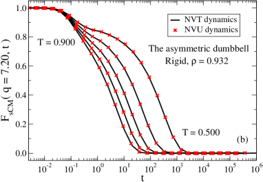
Figure 2: Comparison of structure and dynamics in NVU and NVT simulations of the rigid asymmetric dumbbell model. The black circles and curves give NVT, the red crosses NVU simulation results. (a) The molecular CM radial distribution functions at $\rho$ = 0.932 and T = 0.500. (b) The molecular CM incoherent intermediate scattering functions at $\rho$ = 0.932 and T = 0.500, 0.600, 0.700, 0.800, 0.900.

For reference, we also simulated (Fig. 3) the corresponding quantities for the flexible-bond asymmetric dumbbell model at the state points of Fig. 2. Again, there is a very good agreement between NVU and NVT dynamics.

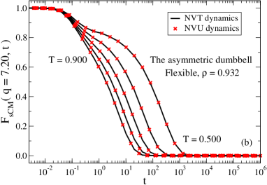
Figure 3: Comparison of structure and dynamics in NVU and NVT simulations of the flexible-bond asymmetric dumbbell model. The black circles and curves give NVT, the red crosses NVU simulation results. The same state points as in Fig. 2 were simulated. (a) The molecular CM radial distribution functions at $\rho$ = 0.932 and T = 0.500. (b) The molecular CM incoherent intermediate scattering functions at $\rho$ = 0.932 and T = 0.500, 0.600, 0.700, 0.800, 0.900.

V.2 Lewis-Wahnström OTP

We show in Figs. 4(a) and (b), respectively, the molecular CM radial distribution functions and CM incoherent intermediate scattering functions for the Lewis-Wahnström OTP model²⁷. The same symbols and meanings as in the preceding section are used. Again, the NVU and NVT simulations agree very well for both structure and dynamics.

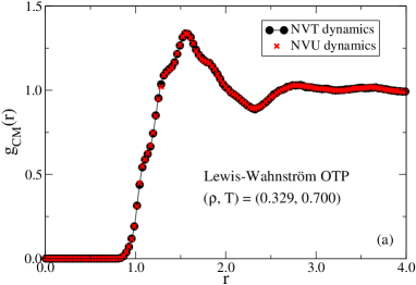
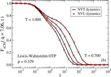
Figure 4: Comparison of center-of-mass structure and dynamics in NVU and NVT simulations of the Lewis-Wahnström OTP model. The black circles and curves give NVT, the red crosses NVU simulation results. (a) The molecular CM radial distribution functions at $\rho$ = 0.329 and T = 0.700. (b) The molecular CM incoherent intermediate scattering functions at $\rho$ = 0.329 and T = 0.700, 0.800, 0.900, 1.000.

For comparison, we also show in Fig. 5 the corresponding particle quantities for the OTP model.

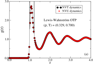
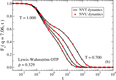
Figure 5: Comparison of particle structure and dynamics in NVU and NVT simulations for the Lewis-Wahnström OTP model. The black circles and curves give NVT, the red crosses NVU simulation results. (a) The particle radial distribution function at $\rho$ = 0.329 and T = 0.700. (b) The particle incoherent intermediate scattering functions at $\rho$ = 0.329 and T = 0.700, 0.800, 0.900, 1.000.

V.3 SPC/E Water

Finally, we consider in Fig. 6 the same quantities as above for the rigid SPC/E water model²⁸. Again, full equivalence between NVU and NVT dynamics is found.

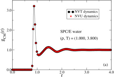
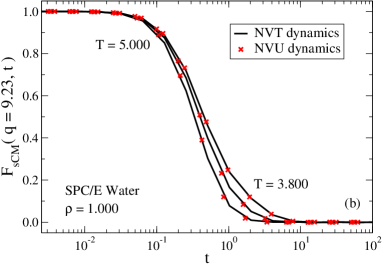
Figure 6: Comparison of structure and dynamics in NVU and NVT simulations of rigid SPC/E water. The black circles and curves give NVT, the red crosses NVU simulation results. (a) The molecular CM radial distribution functions at $\rho$ = 1.000 and T = 3.800. (b) The molecular CM incoherent intermediate scattering functions at $\rho$ = 1.000 and T = 3.800, 4.200, 5.000.

The linear algorithm for determining the Lagrangian multipliers presented in Sec. II.2 (Eqs. (29) and (30)) is tested in Fig. 7 by probing the molecular CM radial distribution functions. NVU and NVT dynamics also here give identical results.

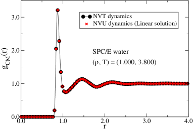
Figure 7: Comparison of structure in NVU and NVT simulations of rigid SPC/E water at $\rho$ = 1.000 and T = 3.800 applying the linear method to determine the Lagrangian multipliers (Eqs. (29) and (30)). The bond lengths are here conserved to order $10^{-6}$ in the standard deviation of the bonds (using single-precision).

We conclude from the presented results that for sufficiently large molecular systems with flexible and/or rigid bonds, NVU dynamics is equivalent to Nosé-Hoover NVT dynamics (and, by implication, Newtonian NVE dynamics).

VI Summary

NVU dynamics is molecular dynamics at constant potential energy realized by tracing out a geodesic on the constant-potential-energy hypersurface $\Omega$ (Eq. (1)). In Papers I and II^{1; 2}, a ”basic” and a ”stabilized” atomic NVU algorithm for simulating geodesics on $\Omega$ was developed. The basic NVU algorithm has excellent stability; it is time-reversible and symplectic, and the stabilized algorithm was developed only to prevent accumulation of numerical error. It was found that atomic NVU dynamics becomes equivalent to atomic NVE dynamics in the thermodynamic limit.

In this paper the stabilized NVU algorithm has been extended to simulate molecules at constant potential energy. Molecules are simulated by introducing rigid and/or flexible bonds in the models. The atomic NVU algorithm keeps the potential energy constant and can thus right away simulate flexible bonds. The focus here was on incorporating rigid bonds in the framework of NVU dynamics, which leads to the introduction of additional Lagrangian multipliers beyond those of the constraint of constant potential energy. This is completely analogous to the approach for simulating rigid bonds in standard Newtonian NVE dynamics^{30; 35; 36}. In the NVU algorithm, a set of coupled quadratic equations was constructed for calculating the Lagrangian multipliers and solved in an iterative manner as a linear system, a procedure developed for rigid-bond NVE dynamics in the MILC-SHAKE algorithm³⁷. In addition, a set of linear equations was presented for calculating the Lagrangian multipliers, and appears to be a promising new way of simulating rigid bonds.

The rigid-bond NVU algorithm reduces to the atomic NVU algorithm when there are no rigid bonds. The algorithm was tested on three different model systems: the asymmetric dumbbell model, Lewis-Wahnström OTP, and rigid SPC/E water. The probed quantities in the simulation gave identical results to those of Nos$\acute{e}$-Hoover NVT dynamics. We conclude that also for molecular systems do NVU dynamics become equivalent to NVE dynamics in the thermodynamic limit (since NVE and NVT dynamics are known to give equivalent results²⁹).

Appendix A Derivation of the atomic NVU algorithm for the Hertzian metric

According to Newtonian dynamics, heavy particles move slower than light particles in thermal equilibrium. The standard Euclidean metric does not involve the particle masses, and thus applying this metric to geodesic motion for systems of varying masses will not produce dynamics equivalent to Newtonian dynamics in a thermal system. The mass-weighted metric of Hertz³², however, ensures that NVU dynamics becomes equivalent to NVE dynamics in the thermodynamic limit, as is clear from the derivation below. This metric is given by (where $\tilde{m}_{k}=m_{k}/\langle m\rangle$)

$$dl^{2}\equiv\sum_{k}\tilde{m}_{k}\big{(}d{\bf r}^{(k)}\big{)}^{2}.$$ (33)

We here derive the discrete NVU algorithm applying the Hertzian metric (this appendix also corrects a typo in Eq. (A5) of Paper II). The discretized variational condition for geodesic motion on $\Omega$ is

$$\delta\left(\sum_{i}\sqrt{\sum_{k}\tilde{m}_{k}\left(\textbf{r}_{i}^{(k)}-\textbf{r}_{i-1}^{(k)}\right)^{2}}-\sum_{i}\lambda_{i}U({\bf R}_{i})\right)\,=\,0\,.$$ (34)

Assuming a constant step length $l_{0}$, i.e.,

$$\sum_{k}\tilde{m}_{k}\left(\textbf{r}_{i}^{(k)}-\textbf{r}_{i-1}^{(k)}\right)^{2}\equiv l_{0}^{2},$$ (35)

it follows by differentiation with respect to $\textbf{r}_{i}^{(k)}$ from Eq. (34) that

$$\tilde{m}_{k}\big{(}\textbf{r}_{i}^{(k)}-\textbf{r}_{i-1}^{(k)}\big{)}+\tilde{m}_{k}\big{(}\textbf{r}_{i}^{(k)}-\textbf{r}_{i+1}^{(k)}\big{)}+l_{0}\lambda_{i}\textbf{f}_{i}^{(k)}\,=\,0.$$ (36)

Defining $\textbf{a}^{(k)}_{i}\equiv(\textbf{r}_{i}^{(k)}-\textbf{r}_{i-1}^{(k)})$ and $\textbf{b}^{(k)}_{i}\equiv(\textbf{r}_{i}^{(k)}-\textbf{r}_{i+1}^{(k)})$, Eq. (35) expresses that $\sum_{k}\tilde{m}_{k}((\textbf{a}^{(k)}_{i})^{2}-(\textbf{b}^{(k)}_{i})^{2})$ = $\sum_{k}\tilde{m}_{k}(\textbf{a}^{(k)}_{i}+\textbf{b}^{(k)}_{i})(\textbf{a}^{(k)}_{i}-\textbf{b}^{(k)}_{i})$ = 0, and thus via Eq. (36)

$$\sum_{k}\tilde{m}_{k}\big{(}-l_{0}/\tilde{m}_{k}\lambda_{i}\textbf{f}_{i}^{(k)}\big{)}\big{(}\textbf{r}^{(k)}_{i+1}-\textbf{r}^{(k)}_{i-1}\big{)}=0.$$ (37)

Equivalently,

$$\sum_{k}\textbf{f}_{i}^{(k)}\textbf{r}^{(k)}_{i+1}=\sum_{k}\textbf{f}_{i}^{(k)}\textbf{r}^{(k)}_{i-1}.$$ (38)

Combining Eq. (38) with the discrete NVU algorithm (Eq. (36)) gives the following result

$$l_{0}\lambda_{i}=\frac{-2\sum_{k}\textbf{f}_{i}^{(k)}\cdot(\textbf{r}^{(k)}_{i}-\textbf{r}^{(k)}_{i-1})}{\sum_{k}\frac{(\textbf{f}_{i}^{(k)})^{2}}{\tilde{m}_{k}}}.$$ (39)

The atomic NVU algorithm with varying masses is thus given by

$$\textbf{r}_{i+1}^{(k)}=2\textbf{r}_{i}^{(k)}-\textbf{r}_{i-1}^{(k)}+\frac{l_{0}}{\tilde{m}_{k}}\lambda_{i}\textbf{f}_{i}^{(k)},$$ (40)

$$l_{0}\lambda_{i}=\frac{-2\sum_{k}\textbf{f}_{i}^{(k)}\cdot(\textbf{r}^{(k)}_{i}-\textbf{r}^{(k)}_{i-1})}{\sum_{k}\frac{(\textbf{f}_{i}^{(k)})^{2}}{\tilde{m}_{k}}}.$$ (41)

References

• (1) T. S. Ingebrigtsen, S. Toxvaerd, O. J. Heilmann, T. B. Schrøder, and J. C. Dyre, J. Chem. Phys. 135, 104101 (2011). (Paper I)
• (2) T. S. Ingebrigtsen, S. Toxvaerd, T. B. Schrøder, and J. C. Dyre, J. Chem. Phys. 135, 104102 (2011). (Paper II)
• (3) R. M. J. Cotterill, Phys. Rev. B 33, 262 (1986)
• (4) R. M. J. Cotterill and J. U. Madsen, Characterizing Complex Systems (Ed. H. Bohr, World Scientific, Singapore, 1990, 177)
• (5) J. L. E. Platt, B. Waszkowycz, R. Cotterill, and B. Robson, Biophys. Chem. 43, 221 (1992)
• (6) R. M. J. Cotterill and J. U. Madsen, J. Phys.: Condens. Matter 18, 6507 (2006)
• (7) A. Scala, L. Angelani, R. D. Leonardo, G. Ruocco, and F. Sciortino, Phil. Mag. B. 82, 151 (2002)
• (8) C. Wang and R. M. Stratt, J. Chem. Phys. 127, 224503 (2007)
• (9) C. Wang and R. M. Stratt, J. Chem. Phys. 127, 224504 (2007)
• (10) C. N. Nguyen and R. M. Stratt, J. Chem. Phys. 133, 124503 (2010)
• (11) C. N. Nguyen, J. I. Isaacson, K. B. Shimmyo, A. Chen, and R. M. Stratt, J. Chem. Phys. 136, 184504 (2012)
• (12) N. P. Bailey, U. R. Pedersen, N. Gnan, T. B. Schrøder, and J. C. Dyre, J. Chem. Phys. 128, 184507 (2008a)
• (13) N. P. Bailey, U. R. Pedersen, N. Gnan, T. B. Schrøder, and J. C. Dyre, J. Chem. Phys. 128, 184508 (2008b)
• (14) T. B. Schrøder, N. P. Bailey, U. R. Pedersen, N. Gnan, and J. C. Dyre, J. Chem. Phys. 131, 234503 (2009)
• (15) N. Gnan, T. B. Schrøder, U. R. Pedersen, N. P. Bailey, and J. C. Dyre, J. Chem. Phys. 131, 234504 (2009)
• (16) T. B. Schrøder, N. Gnan, U. R. Pedersen, N. P. Bailey, and J. C. Dyre, J. Chem. Phys. 134, 164505 (2011)
• (17) T. S. Ingebrigtsen, T. B. Schrøder, and J. C. Dyre, J. Phys. Chem. B 116, 1018 (2012)
• (18) T. S. Ingebrigtsen, L. Bøhling, T. B. Schrøder, and J. C. Dyre, J. Chem. Phys. 136, 061102 (2012)
• (19) T. S. Ingebrigtsen, T. B. Schrøder, and J. C. Dyre, Phys. Rev. X. 2, 011011 (2012)
• (20) J. E. Marsden and M. West, Acta Numer. 10, 357 (2001)
• (21) R. Elber, A. Cardenas, A. Ghosh, and H. A. Stern, Adv. Chem. Phys. 93, 126 (2003)
• (22) A. Lew, Variational time integrators in computational solid mechanics, Ph.D. thesis, California Institute of Technology (2003)
• (23) M. West, Variational integrators, Ph.D. thesis, California Institute of Technology (2004)
• (24) S. NosĂŠ, J. Chem. Phys. 81, 511 (1984)
• (25) W. G. Hoover, Phys. Rev. A 31, 1695 (1985)
• (26) T. B. Schrøder, U. R. Pedersen, N. P. Bailey, S. Toxvaerd, and J. C. Dyre, Phys. Rev. E 80, 041502 (2009)
• (27) L. J. Lewis and G. WahnstrĂśm, Phys. Rev. E 50, 3865 (1994)
• (28) H. J. C. Berendsen, J. R. Grigera, and T. P. Straatsma, J. Phys. Chem. 91, 6269 (1987)
• (29) D. J. Evans and B. L. Holian, J. Chem. Phys. 83, 4069 (1985)
• (30) J. P. Ryckaert, G. Ciccotti, and H. J. C. Berendsen, J. Comput. Phys. 23, 327 (1977)
• (31) H. Goldstein, C. Poole, and J. Safko, Classical Mechanics, 3rd ed. (Addison Wesley, 2002)
• (32) H. Hertz, Die Prinzipien der Mechanik, in Neuem Zusammenhange Dargestellt (Johann Ambrosius Barth, Leipzig, 1894)
• (33) J. LĂźtzen, Mechanistic Images in Geometric Form: Heinrich Hertz’s ”Principles of Mechanics” (Oxford University Press, Oxford, 2005)
• (34) M. P. Allen and D. J. Tildesley, Computer Simulation of Liquids (Oxford Science Publications, 1987)
• (35) S. Toxvaerd, O. J. Heilmann, T. Ingebrigtsen, T. B. Schrøder, and J. C. Dyre, J. Chem. Phys. 131, 064102 (2009)
• (36) T. Ingebrigtsen, O. J. Heilmann, S. Toxvaerd, and J. C. Dyre, J. Chem. Phys 132, 154106 (2010)
• (37) A. G. Bailey, C. P. Lowe, and A. P. Sutton, J. Comput. Phys. 227, 8949 (2008)
• (38) S. Toxvaerd and J. C. Dyre, J. Chem. Phys. 134, 081102 (2011a)
• (39) “All simulations were performed using a molecular dynamics code optimized for NVIDIA graphics cards, which is available as open source code at http://rumd.org,”
• (40) S. Toxvaerd, Mol. Phys. 72, 159 (1991)
• (41) N. Bell and M. Garland, “Cusp: Generic parallel algorithms for sparse matrix and graph computations,”  (2012), version 0.3.0, http://cusp-library.googlecode.com
• (42) W. H. Press, S. A. Teukolsky, W. T. Vetterling, and B. P. Flannery, Numerical Recipes, 3rd ed. (Cambridge University Press, 2007)
• (43) C. J. Fennell and J. D. Gezelter, J. Chem. Phys. 124, 234104 (2006)
• (44) J. S. Hansen, T. B. Schrøder, and J. C. Dyre, J. Phys. Chem. B 116, 5738 (2012)