Search trees: Metric aspects and strong limit theorems

Abstract

We consider random binary trees that appear as the output of certain standard algorithms for sorting and searching if the input is random. We introduce the subtree size metric on search trees and show that the resulting metric spaces converge with probability 1. This is then used to obtain almost sure convergence for various tree functionals, together with representations of the respective limit random variables as functions of the limit tree.

60B99, 60J10, 68Q25, 05C05, Doob-Martin compactification, metric trees, path length, silhouette, subtree size metric, vector-valued martingales, Wiener index

1 Introduction

A sequential algorithm transforms an input sequence $t_{1},t_{2},\ldots$ into an output sequence $x_{1},x_{2},\ldots$ where, for all $n\in\mathbb{N}$, $x_{n+1}$ depends on $x_{n}$ and $t_{n+1}$ only. Typically, the output variables are elements of some combinatorial family $\mathbb{F}$, each $x\in\mathbb{F}$ has a size parameter $\phi(x)\in\mathbb{N}$ and $x_{n}$ is an element of the set $\mathbb{F}_{n}:=\{x\in\mathbb{F}\dvtx\phi(x)=n\}$ of objects of size $n$. In the probabilistic analysis of such algorithms, one starts with a stochastic model for the input sequence and is interested in certain aspects of the output sequence. The standard input model assumes that the $t_{i}$’s are the values of a sequence $\eta_{1},\eta_{2},\ldots$ of independent and identically distributed random variables. For random input of this type, the output sequence then is the path of a Markov chain $X=(X_{n})_{n\in\mathbb{N}}$ that is adapted to the family $\mathbb{F}$ in the sense that

$$P(X_{n}\in\mathbb{F}_{n})=1\qquad\mbox{for all }n\in\mathbb{N}.$$ (1)

Clearly, $X$ is highly transient—no state can be visited twice.

The special case we are interested in, and which we will use to demonstrate an approach that is generally applicable in the situation described above, is that of binary search trees and two standard algorithms, known by their acronyms BST (binary search tree) and DST (digital search tree). These are discussed in detail in the many excellent texts in this area, for example in Knuth3 , Mahmoud1 and Drmota09 . Various functionals of the search trees, such as the height Dev86 , the path length RegnierQS , RoeQS , the node depth profile J-H2001 , CDJ2001 , CR2004 , CKMR2005 , FHN2006 , DJN2008 , the subtree size profile Fu2008 , DeGr3 , the Wiener index Nein02 and the silhouette GrSilh have been studied, with methods spanning the wide range from generatingfunctionology to martingale methods to contraction arguments on metric spaces of probability distributions (neither of these lists is complete). Many of the results are asymptotic in nature, where the convergence obtained as $n\to\infty$ may refer to the distributions or to the random variables themselves. As far as strong limit theorems are concerned, a significant step toward a unifying approach was made in the recent paper EGW , where methods from discrete potential theory were used to obtain limit results on the level of the combinatorial structures themselves: In a suitable extension of the state space $\mathbb{F}$, the random variables $X_{n}$ converge almost surely as $n\to\infty$, and the limit generates the tail $\sigma$-field of the Markov chain. The results in EGW cover a wide variety of structures; search trees are a special case. It should also be mentioned here that the use of boundary theory has a venerable tradition in connection with random walks; see KaimVersh and Woess1 .

Our aims in the present paper are the following. First, we use the algorithmic background for a direct proof of the convergence of the BST variables $X_{n}$, as $n\to\infty$, to a limit object $X_{\infty}$, and we obtain a representation of $X_{\infty}$ in terms of the input sequence $(\eta_{i})_{i\in\mathbb{N}}$. Second, we introduce the subtree size metric on finite binary trees. This leads to a reinterpretation of the above convergence in terms of metric trees. We also introduce a family of weighted variants of this metric, with parameter $\rho\geq 1$, and then identify the critical value $\rho_{0}$ with the property that the metric trees converge for $\rho<\rho_{0}$ and do not converge if $\rho>\rho_{0}$. The value $\rho_{0}$ turns out to also be the threshold for compactness of the limit tree. Third, we use convergence at the tree level to (re)obtain strong limit theorems for three tree functionals—the path length, the Wiener index and a metric version of the silhouette.

These topics are treated in the next three sections, where each has its own introductory remarks.

2 Binary search trees

We first introduce some notation, mostly specific to binary trees, then discuss the two search algorithms and the associated Markov chains and finally recall the results from EGW related to these structures, including an alternative proof of the main limit theorem.

2.1 Some notation

We write $\mathcal{L}(X)$ for the distribution of a random variable $X$ and $\mathcal{L}(X|Y=k)$, $\mathcal{L}(X|Y)$, $\mathcal{L}(X|\mathcal{F})$ for the various versions of the conditional distribution of $X$ given (the value of) a random variable $Y$ or a $\sigma$-field $\mathcal{F}$. Further, $\delta_{c}$ is the one-point mass at $c$, $1_{A}$ is the indicator function of the set $A$ [so that $1_{A}(c)=\delta_{c}(A)$], $\operatorname{Bin}(n,p)$ denotes the binomial distribution with parameters $n\in\mathbb{N}$ and $p\in(0,1)$, $\operatorname{Beta}(\alpha,\beta)$ is the beta distribution with parameters $\alpha,\beta>0$ and $\operatorname{unif}(0,1)=\operatorname{Beta}(1,1)$ is the uniform distribution on the unit interval. We also write $\operatorname{unif}(M)=(\#M)^{-1}\sum_{c\in M}\delta_{c}$ for the uniform distribution on a finite set $M$.

With $\mathbb{N}_{0}=\{0,1,2,\ldots\}$ let

$$\mathbb{V}_{k}:=\{0,1\}^{k},\qquad\mathbb{V}:=\bigsqcup_{k\in\mathbb{N}_{0}}\mathbb{V}_{k},\qquad\partial\mathbb{V}:=\{0,1\}^{\infty}$$

be the set of 0–1 sequences of length $k$, $k\in\mathbb{N}_{0}$, the set of all finite 0–1 sequences and the set of all infinite 0–1 sequences, respectively. The set $\mathbb{V}_{0}$ has $\varnothing$, the “empty sequence,” as its only element, and $|u|$ is the length of $u\in\mathbb{V}$, that is, $|u|=k$ if $u\in\mathbb{V}_{k}$. For each node $u=(u_{1},\ldots,u_{k})\in\mathbb{V}$ we use

$$u0 := (u_{1},\ldots,u_{k},0),$$

$$u1 := (u_{1},\ldots,u_{k},1),$$

$$\bar{u} := (u_{1},\ldots,u_{k-1})\qquad\mbox{if }k\geq 1,$$

to denote its left and right direct descendant (child) and its direct ancestor (parent). We write $u\leq v$ for $u=(u_{1},\ldots,u_{k})\in\mathbb{V}$, $v=(v_{1},\ldots,v_{l})\in\mathbb{V}$ if $k\leq l$ and $u_{j}=v_{j}$ for $j=1,\ldots,k$, that is, if $u$ is a prefix of $v$; the extension to $v\in\partial\mathbb{V}$ is obvious. The prefix order is a partial order only, but there exists a unique minimum $u\wedge v$ to any two nodes $u,v\in\mathbb{V}$, their last common ancestor; again, this can be extended to elements of $\partial\mathbb{V}$. Another ordering on $\mathbb{V}$ can be obtained via the function $\beta\dvtx\mathbb{V}\to[0,1]$,

$$\beta(u):=\frac{1}{2}+\sum_{j=1}^{k}\frac{2u_{j}-1}{2^{j+1}},\qquad u\in\mathbb{V}.$$ (2)

This will be useful in various proofs, and also in connection with illustrations.

By a binary tree we mean a subset $x$ of the set $\mathbb{V}$ of nodes that is prefix stable in the sense that $u\in x$ and $v\leq u$ implies that $v\in x$. Informally, we regard the components $u_{1},\ldots,u_{k}$ of $u$ as a routing instruction leading to the vertex $u$, where 0 means a move to the left, 1 a move to the right and the empty sequence is the root node. The edges of the tree $x$ are the pairs $(\bar{u},u)$, $u\in x,u\neq\varnothing$. A node is external to a tree if it is not one of its elements, but its direct ancestor is; we write $\partial x:=\{u\in\mathbb{V}\dvtx\bar{u}\in x,u\notin x\}$ for the set of external nodes of $x$. Finally,

$$\sigma(x,u):=\#\{v\in x\dvtx u\leq v\}$$ (3)

is the size of the subtree of $x$ rooted at $u$ (or the number of descendants of $u$ in $x$, including $u$).

Let $\mathbb{B}$ denote the (countable) set of finite binary trees, $\mathbb{B}_{n}:=\{x\in\mathbb{B}\dvtx\#x=n\}$ those of size (number of nodes) $n$. The single element of $\mathbb{B}_{1}$ is $\{\varnothing\}$, the tree that consists of the root node only.

2.2 Search algorithms and Markov chains

Let $(t_{i})_{i\in\mathbb{N}}$ be a sequence of pairwise distinct real numbers. The BST (binary search tree) algorithm stores these sequentially into labeled binary trees $(x_{n},L_{n})$, $n\in\mathbb{N}$, with $x_{n}\in\mathbb{B}_{n}$ and $L_{n}\dvtx x_{n}\to\{t_{1},\ldots,t_{n}\}$. For $n=1$ we have $x_{1}=\{\varnothing\}$ and $L_{1}(\varnothing)=t_{1}$. Given $(x_{n},L_{n})$, we construct $(x_{n+1},L_{n+1})$ as follows: Starting at the root node we compare the next input value $t_{n+1}$ to the value $L_{n}(u)$ attached to the node $u$ under consideration, and move to $u0$ if $t_{n+1}<L_{n}(u)$ and to $u1$ otherwise, until an “empty” node $u$ (necessarily an external node of $x_{n}$) is found. Then $x_{n+1}:=x_{n}\cup\{u\}$ and $L_{n+1}(u):=t_{n+1}$, $L_{n+1}(v):=L_{n}(v)$ for all $v\in x_{n}$.

Now let $(\eta_{i})_{i\in\mathbb{N}}$ be a sequence of independent random variables with $\mathcal{L}(\eta_{i})=\operatorname{unif}(0,1)$ for all $i\in\mathbb{N}$, and let $X_{n}$ be the random binary tree associated with the first $n$ of these. By construction, the label functions $L_{n}$ are monotone with respect to the $\beta$-order of the tree nodes, that is, with $\beta$ as in (2),

$$\beta(u)\leq\beta(v)\Rightarrow L_{n}(u)\leq L_{n}(v)\qquad\mbox{for all }n\mbox{ with }\{u,v\}\subset X_{n}.$$ (4)

In particular, if we number the external nodes of $X_{n}$ from the left to the right, then the number of the node that receives $\eta_{n+1}$ is the rank of this value among $\{\eta_{1},\ldots,\eta_{n}\}$, hence uniformly distributed on $\{1,\ldots,n+1\}$. This shows that the (deterministic) BST algorithm, when applied to the (random) input $(\eta_{i})_{i\in\mathbb{N}}$, results in a Markov chain $(X_{n})_{n\in\mathbb{N}}$ with state space $\mathbb{B}$, start at $X_{1}\equiv\{\varnothing\}$ and transition probabilities

$$Q\bigl{(}x,x\cup\{u\}\bigr{)}=\cases{1/(1+\#x),&\quad$\mbox{if }u\in\partial x$,\vspace*{2pt}\cr 0,&\quad$\mbox{otherwise}$.}$$ (5)

In words: We obtain $X_{n+1}$ by choosing one of the $n+1$ external nodes of $X_{n}$ uniformly at random and joining it to the tree. We refer to this construction as the BST chain.

For the DST (digital search tree) algorithm, the input values are infinite 0–1 sequences, that is, elements of $\partial\mathbb{V}$. Given $t_{1},t_{2},\ldots\in\partial\mathbb{V}$ we again obtain a sequence $x_{1},x_{2},\ldots$ of labeled binary trees, but now we use the components $t_{n+1,k}$, $k\in\mathbb{N}$, of the next input value $t_{n+1}$ as a routing instruction through $x_{n}$, moving to $u0$ from an occupied node $u\in\mathbb{V}_{k}$ if $t_{n+1,k+1}=0$ and to $u1$ otherwise. As in the BST case we assume that the $t_{i}$’s are the values of a sequence of independent and identically distributed random variables $\eta_{i}$, where the distribution of the $\eta_{i}$’s is now a probability measure $\mu$ on the measurable space $(\partial\mathbb{V},\mathcal{B}(\partial\mathbb{V}))$, with $\mathcal{B}(\partial\mathbb{V})$ the $\sigma$-field generated by the projections on the sequence elements, $\partial\mathbb{V}\ni t=(t_{k})_{k\in\mathbb{N}}\mapsto t_{i}$, $i\in\mathbb{N}$. This $\sigma$-field is also generated by the sets

$$A_{u}:=\{v\in\partial\mathbb{V}\dvtx v\geq u\},\qquad u\in\mathbb{V}.$$ (6)

It is easy to check that the intersection of two such sets is either empty or again of this form. This implies that $\mu$ is completely specified by its values $\mu(A_{u})$, $u\in\mathbb{V}$, and the DST analogue of (5) then is

$$Q\bigl{(}x,x\cup\{u\}\bigr{)}=\cases{\mu(A_{u}),&\quad$\mbox{if }u\in\partial x$,\vspace*{2pt}\cr 0,&\quad$\mbox{otherwise}$.}$$ (7)

By the DST chain with driving distribution $\mu$ we mean a Markov chain $(X_{n})_{n\in\mathbb{N}}$ with state space $\mathbb{B}$, start at $\{\varnothing\}$ and transition mechanism given by (7).

2.3 Doob–Martin compactification

We refer the reader to Doob’s seminal paper Doob1959 and to the recent textbook Woess2 for the main results of, background on and further references for the boundary theory for transient Markov chains. For the BST chain the Doob–Martin compactification has recently been obtained in EGW : It can be described as the closure $\bar{\mathbb{B}}$ of the embedding of $\mathbb{B}$ into the compact space $[0,1]^{\mathbb{V}}$, endowed with pointwise convergence, that is given by the standardized subtree size functional

$$\mathbb{B}\ni x\mapsto\biggl{(}\mathbb{V}\ni u\mapsto\frac{\sigma(x,u)}{\#x}\biggr{)}$$

with $\sigma$ as defined in (3). Further, the elements of the boundary $\partial\mathbb{B}$ may be represented by probability measures $\mu$ on $(\partial\mathbb{V},\mathcal{B}(\partial\mathbb{V}))$, with convergence $x_{n}\to\mu$ of a sequence $(x_{n})_{n\in\mathbb{N}}$ in $\mathbb{B}$ meaning that

$$\mu(A_{u})=\lim_{n\to\infty}\frac{\sigma(x_{n},u)}{\#x_{n}}\qquad\mbox{for all }u\in\mathbb{V},$$

and $\mu_{n}(A_{u})\to\mu(A_{u})$ for all $u\in\mathbb{V}$ if we have a sequence $(\mu_{n})_{n\in\mathbb{N}}$ of elements of $\partial\mathbb{B}$ instead.

The general theory implies that $X_{n}$ converges almost surely to a limit $X_{\infty}$ with values in $\partial\mathbb{B}$; EGW also contains a description of $\mathcal{L}(X_{\infty})$. The proof given there does not make use of the algorithmic background, but takes the transition mechanism (5) as its starting point. We now show that this background leads to a direct proof of $X_{n}\to X_{\infty}$, and to a representation of $X_{\infty}$ in terms of the input sequence.

We need some more notation. On $\mathbb{V}$ we define a metric $d_{\mathbb{V}}$ by

$$d_{\mathbb{V}}(u,v):=2^{-|u\wedge v|}-\tfrac{1}{2}\bigl{(}2^{-|u|}+2^{-|v|}\bigr{)},\qquad u,v\in\mathbb{V}.$$ (8)

On $\mathbb{V}$ itself this gives the discrete topology, and the completion of $\mathbb{V}$ with respect to $d_{\mathbb{V}}$ leads to $\bar{\mathbb{V}}:=\mathbb{V}\cup\partial\mathbb{V}$, a compact and separable metric space. This is also the ends compactification if we regard $\mathbb{V}$ as the complete rooted binary tree. We extend the $A_{u}$’s to $\bar{\mathbb{V}}$ by

$$\bar{A}_{u}:=\{v\in\bar{\mathbb{V}}\dvtx v\geq u\},\qquad u\in\mathbb{V}.$$

Because of

$$\bar{A}_{u}:=\bigl{\{}v\in\bar{\mathbb{V}}\dvtx d_{\mathbb{V}}(u,v)<2^{-|u|}\bigr{\}}=\bigl{\{}v\in\bar{\mathbb{V}}\dvtx d_{\mathbb{V}}(u,v)\leq 2^{-|u|-1}\bigr{\}}$$

these sets are open and closed. Further,

$$\{u\}=\bar{A}_{u}\setminus(\bar{A}_{u0}\cup\bar{A}_{u1}),\qquad\bar{A}_{u}\cap\bar{A}_{v}=\cases{\bar{A}_{u},&\quad$\mbox{if }u\leq v$,\vspace*{2pt}\cr\bar{A}_{v},&\quad$\mbox{if }u\geq v$,\vspace*{2pt}\cr\varnothing,&\quad$\mbox{otherwise,}$}$$

hence $\{\bar{A}_{u}\dvtx u\in\mathbb{V}\}$ is a $\pi$-system that generates $\mathcal{B}(\bar{\mathbb{V}})$. Together these facts imply that weak convergence of probability measures $\mu_{n}$ to a probability measure $\mu$ on $(\bar{\mathbb{V}},\mathcal{B}(\bar{\mathbb{V}}))$ is equivalent to

$$\lim_{n\to\infty}\mu_{n}(\bar{A}_{u})=\mu(\bar{A}_{u})\qquad\mbox{for all }u\in\mathbb{V}.$$ (9)

In view of

$$\frac{1}{n}\sigma(X_{n},u)=\operatorname{unif}(X_{n})(\bar{A}_{u})$$

and $X_{\infty}(\mathbb{V})=0$ convergence in the Doob–Martin topology is therefore equivalent to the weak convergence of probability measures on the metric space $(\bar{\mathbb{V}},d_{\mathbb{V}})$ if we represent finite subsets $M$ of $\mathbb{V}$ by the uniform distribution $\operatorname{unif}(M)$ on $(\bar{\mathbb{V}},\mathcal{B}(\bar{\mathbb{V}}))$.

Moreover, any sequence $(\mu_{n})_{n\in\mathbb{N}}$ of probability measures on $(\bar{\mathbb{V}},\mathcal{B}(\bar{\mathbb{V}}))$ is tight, as $\bar{\mathbb{V}}$ is compact, and therefore has a limit point by Prohorov’s theorem Bill68 , page 37. If $(\mu_{n}(\bar{A}_{u}))_{n\in\mathbb{N}}$ is a convergent sequence for each $u\in\mathbb{V}$, then there is only one such limit point, which means that $\mu_{n}$ converges weakly to some probability measure $\mu$ and that (9) holds. Finally, let

$$\tau(u):=\inf\{n\in\mathbb{N}\dvtx X_{n}\ni u\},\qquad u\in\mathbb{V},$$ (10)

be the time that the node $u$ becomes an element of the BST sequence. It is easy to see that the $\tau(u)$’s are finite with probability 1.

Theorem 1

Let $(X_{n})_{n\in\mathbb{N}}$ be the sequence of binary trees generated by the BST algorithm with input a sequence $(\eta_{i})_{i\in\mathbb{N}}$ of independent and identically distributed random variables with $\mathcal{L}(\eta_{1})=\operatorname{unif}(0,1)$.

[(a)]

With probability 1 the sequence $\operatorname{unif}(X_{n})$ converges weakly to a random probability measure $X_{\infty}$ on $(\partial\mathbb{V},\mathcal{B}(\partial\mathbb{V}))$ as $n\to\infty$.

For each $u\in\mathbb{V}$, $u\neq\varnothing$, with $i:=\tau(u)-1$, $\tau$ as in (10), and

$$0=:\eta_{(i:0)}<\eta_{(i:1)}<\cdots<\eta_{(i:i)}<\eta_{(i:i+1)}:=1$$

the augmented order statistics associated with $\eta_{1},\ldots,\eta_{i}$, we have

$$X_{\infty}(A_{u})=\eta_{(i:j+1)}-\eta_{(i:j)}\qquad\mbox{with }\eta_{(i:j)}<\eta_{i+1}<\eta_{(i:j+1)}.$$

The random variables

$$\xi_{u}:=\frac{X_{\infty}(A_{u0})}{X_{\infty}(A_{u})},\qquad u\in\mathbb{V},$$

are independent, and $\mathcal{L}(\xi_{u})=\operatorname{unif}(0,1)$ for all $u\in\mathbb{V}$.

Let $u$, $\tau(u)$, $i$ and $\eta_{(i:j)}$, $j=0,\ldots,i+1$, be as in part (b) of the theorem. The order property (4) of the labeled binary search trees implies that for a node $v$ with label $\eta_{k}$, $k>i$, the relation $v\geq u$ is equivalent to $\eta_{(i:j)}<\eta_{k}<\eta_{(i:j+1)}$. Hence, by the law of large numbers,

$$\lim_{n\to\infty}\operatorname{unif}(X_{n})(\bar{A}_{u}) = \lim_{n\to\infty}\frac{\#\{v\in X_{n}\dvtx v\geq u\}}{n}$$

$$= \lim_{n\to\infty}\frac{\#\{i<k\leq n\dvtx\eta_{k}\in(\eta_{(i:j)},\eta_{(i:j+1)})\}}{n}$$

$$= \eta_{(i:j+1)}-\eta_{(i:j)}$$

with probability 1 for every $u\in\mathbb{V}$. In view of

$$\{u\}=\bigl{\{}v\in\bar{\mathbb{V}}\dvtx d(u,v)<2^{-|u|-1}\bigr{\}}\qquad\mbox{for all }u\in\mathbb{V},$$

the one-point sets with elements from $\mathbb{V}$ are open in the topology on $\bar{\mathbb{V}}$. As $\operatorname{unif}(X_{n})$ assigns at most the value $1/n$ to such a set, it follows with the portmanteau theorem Bill68 , page 11, that any limit point of this sequence is concentrated on $\partial\mathbb{V}$. Parts (a) and (b) of the theorem now follow with the above general remarks on weak convergence of probability measures on $(\bar{\mathbb{V}},\mathcal{B}(\bar{\mathbb{V}}))$.

For the proof of (c) we use the following well-known fact: The conditional distribution of $\eta_{i+1}$, given $\eta_{1},\ldots,\eta_{i}$ and given that the value lands in an interval $I=(\eta_{(i:j)},\eta_{(i:j+1)})$ of the augmented order statistics, is the uniform distribution on $I$, which implies that $\operatorname{unif}(0,1)$ is the distribution of the normalized distance $\xi_{u}$ to the left endpoint of $I$. For different $\eta$-values these relative insertion positions are independent, hence $\xi_{u}$, $u\in\mathbb{V}$, are independent and uniformly distributed on the unit interval.

We note the following consequence of the representation in part (c) of the theorem: For a fixed $u\in\mathbb{V}$ let

$$\varnothing=u(0)<u(1)<\cdots<u(k)=u$$

with $|u(j)|=j$ for $j=0,\ldots,k$ be the path that connects $u$ to the root node. We then have

$$X_{\infty}(A_{u})=\prod_{j=0}^{k-1}\tilde{\xi}_{u(j)}$$

(11)

$$\eqntext{\displaystyle\mbox{with }\tilde{\xi}_{u(j)}:=\cases{\xi_{u(j)},&\quad$\mbox{if }u(j+1)=u(j)0$,\vspace*{2pt}\cr 1-\xi_{u(j)},&\quad$\mbox{if }u(j+1)=u(j)1$.}}$$ (12)

Note that the factors $\tilde{\xi}_{u(j)}$, $j=0,\ldots,k-1$, are independent and that they all have distribution $\operatorname{unif}(0,1)$.

Theorem 1 confirms the view expressed in Woess2 , pages 191 and 218, that in specific cases embeddings (or boundaries) can generally be obtained directly on using the then available additional structure; here this turns out to be the algorithmic representation of the Markov chain. However, there are two additional benefits of the general theory: First, because of the space–time property (1) the limit $X_{\infty}$ generates the tail $\sigma$-field

$$\mathcal{T}:=\bigcap_{n=1}^{\infty}\sigma\bigl{(}\{X_{m}\dvtx m\geq n\}\bigr{)}$$

associated with the sequence $(X_{n})_{n\in\mathbb{N}}$. This may serve as a starting point for the unification of strong limit theorems for functionals $(Y_{n})_{n\in\mathbb{N}}$, $Y_{n}=\Psi(X_{n})$ of the discrete structures: If $Y_{n}$ converges to $Y_{\infty}$ in a “reasonable” space, then the limit $Y_{\infty}$, which is $\mathcal{T}$-measurable, must be a function of $X_{\infty}$; see, for example, Kall , Lemma 1.13. The second general result is extremely useful in the context of the calculations that arise in specific applications of the theory: The conditional distribution of the chain $(X_{n})_{n\in\mathbb{N}}$ given the value of $X_{\infty}$ is again a Markov chain, where the new transition probabilities can be obtained from the limit value and the old transition probabilities by a procedure that is known as Doob’s $h$-transform. In the present situation it turns out that the conditional distribution of the BST chain, given $X_{\infty}=\mu$, is the same as that of the DST chain driven by $\mu$. We refer the reader to EGW for details; the last statement appears there only for a specific $\mu$, but the generalization to an arbitrary probability measure $\mu$ in the boundary is straightforward. Roughly, the embedded jump chains at the individual nodes are Pólya urns; for these the boundary has been obtained in BK1964 , and from the general construction of the Doob–Martin boundary it is clear that the outcome is unaffected by the step from a Markov chain to its embedded jump chain. We collect some consequences in the following proposition, where

$$\mathcal{F}_{n}:=\sigma(X_{1},\ldots,X_{n}),\qquad n\in\mathbb{N},$$ (13)

are the elements of the natural filtration of the BST chain.

Proposition 2

With the notation and assumptions as in Theorem 1,

$$\mathcal{L}\bigl{(}\sigma(X_{n},u0)|\sigma(X_{n},u)=k,\xi_{u}=p\bigr{)}=\operatorname{Bin}(k-1,p)\qquad\mbox{if }k>0,$$ (14)

and, for all $i,j\in\mathbb{N}_{0}$,

$$\mathcal{L}\bigl{(}\xi_{u}|\sigma(X_{n},u0)=i,\sigma(X_{n},u1)=j\bigr{)}=\operatorname{Beta}(i+1,j+1).$$ (15)

Further, the variables $(\xi_{u})_{u\in\mathbb{V}}$ are conditionally independent given $\mathcal{F}_{n}$.

3 Metric aspects

All trees in this paper are subgraphs of the complete binary tree, which has $\mathbb{V}$ as its set of nodes and $\{(\bar{u},u)\dvtx u\neq\varnothing\}$ as its set of edges; in particular, our trees are specified by their node sets $x$. In a tree metric $d$ the distance of any two nodes $u,v$ is the sum of the distances between successive nodes on the unique path from $u$ to $v$, which means that such a metric is given by its values $d(\bar{u},u)$, $u\in x$, $u\neq\varnothing$. For example, the metric $d_{\mathbb{V}}$ in Section 2.3 has $d_{\mathbb{V}}(\bar{u},u)=2^{-|u|-1}$, and the canonical tree distance $d_{\mathrm{can}}$ is given by $d_{\mathrm{can}}(\bar{u},u)=1$. For our trees the prefix order further leads to

$$d(u,v)=d(u,\varnothing)+d(v,\varnothing)-2d(u\wedge v,\varnothing)\qquad\mbox{for all }u,v\in x.$$ (16)

Metric trees may also be interpreted as graphs with edge weight, where the edge $(\bar{u},u)$ receives the weight $d(\bar{u},u)$.

Our aim in this section is to rephrase the convergence of the BST sequence as a convergence of metric trees, and to show that this view leads to convergence with respect to stronger topologies. The situation here is much simpler than for Aldous’s continuum random tree where the Gromov–Hausdorff convergence of equivalence classes of metric trees is used; see EvansSF and the references given there. In fact, the search trees considered here have node sets that grow monotonically to the full $\mathbb{V}$, so we may define convergence of a sequence $((x_{n},d_{n}))_{n\in\mathbb{N}}$ of metric binary trees to $(\mathbb{V},d_{\infty})$ to mean that

$$\lim_{n\to\infty}d_{n}(u,v)=d_{\infty}(u,v)\qquad\mbox{for all }u,v\in\mathbb{V},$$ (17)

which of course is equivalent to $\lim_{n\to\infty}d_{n}(\bar{u},u)=d_{\infty}(\bar{u},u)$ for all $u\in\mathbb{V}$, $u\neq\varnothing$. Note that $d_{\mathbb{V}}$ and $d_{\mathrm{can}}$ are both local metrics in the sense that $d(u,v)$ does not depend on the tree $x$ as long as $u,v\in x$.

Motivated by the view in Section 2.3 of finite and infinite binary trees as probability measures $\mu$ on $(\bar{\mathbb{V}},\mathcal{B}(\bar{\mathbb{V}}))$, we now introduce the (relative) subtree size metric, which assigns $\mu(\bar{A}_{u})$ to the distance of $\bar{u}$ and $u$, that is,

$$d_{x}(\bar{u},u)=\frac{\sigma(x,u)}{\sigma(x,\varnothing)}\qquad\mbox{for all }u\in x,u\neq\varnothing,$$

if $x\in\mathbb{B}$, and

$$d_{\mu}(\bar{u},u)=\mu(A_{u})\qquad\mbox{for all }u\in\mathbb{V},u\neq\varnothing$$

for the complete tree and a probability measure $\mu$ on $(\partial\mathbb{V},\mathcal{B}(\partial\mathbb{V}))$, where we assume that $\mu(A_{u})>0$ for all $u\in\mathbb{V}$. Again, there is an algorithmic motivation: In terms of the BST mechanism, the weight of an edge $(\bar{u},u)$ is the (relative) number of times this edge has been traversed in the construction of the tree. These metrics depend on their tree in a global manner.

With this terminology in place we may now rephrase the convergence in Theorem 1 as the convergence in the sense of (17) of the finite metric trees $(X_{n},d_{X_{n}})$ to the infinite metric tree $(\mathbb{V},d_{X_{\infty}})$, almost surely and as $n\to\infty$.

By construction the Doob–Martin compactification is the weakest topology that allows for a continuous extension of the functions $\mathbb{B}\ni x\mapsto\sigma(x,u)/\break\sigma(x,\varnothing)$, $u\in\mathbb{V}$. For the analysis of tree functionals stronger modes of convergence turn out to be useful; for example, do we have uniform convergence in (17)? Also, subtree sizes decrease along paths leading away from the root node, so we may consider a weight factor for the distance of a node to its parent that depends on the depth of the node: For all $\rho\geq 1$, we define the weighted subtree size metric with weight parameter $\rho$ by

$$d_{x,\rho}(\bar{u},u):=\rho^{|u|}d_{x}(\bar{u},u),\qquad d_{\mu,\rho}(\bar{u},u):=\rho^{|u|}d_{\mu}(\bar{u},u),$$

in the finite and infinite case, respectively. Of course, with $\rho=1$ the subtree size metric reappears.

Theorem 3

Let $\rho_{0}=1.26107\cdots$ be the smaller of the two roots of the equation $2e\log(\rho)=\rho$, $\rho>0$. Let $X_{n}$, $n\in\mathbb{N}$ and $X_{\infty}$ be as in Theorem 1. [(a)]

For $\rho<\rho_{0}$, the metric space $(\mathbb{V},d_{X_{\infty},\rho})$ is compact with probability 1.

For $\rho>\rho_{0}$, the metric space $(\mathbb{V},d_{X_{\infty},\rho})$ has infinite diameter with probability 1.

For $\rho<\rho_{0}$, the metric spaces $(X_{n},d_{X_{n},\rho})$ converge uniformly to$(\mathbb{V},d_{X_{\infty},\rho})$ as $n\to\infty$ in the sense of

$$\sup_{u,v\in X_{n}}\bigl{|}d_{X_{n},\rho}(u,v)-d_{X_{\infty},\rho}(u,v)\bigr{|}\to 0\qquad\mbox{ almost surely and in mean}.$$ (18)

For $\rho>\rho_{0}$, and with $d_{X_{n},\rho}(\bar{u},u):=0$ for $u\notin X_{n}$,

$$\sup_{u,v\in\mathbb{V}}\bigl{|}d_{X_{n},\rho}(u,v)-d_{X_{\infty},\rho}(u,v)\bigr{|}=\infty\qquad\mbox{with probability 1}.$$

We embed the metric trees into the linear space $\mathbb{L}(0)$ of all functions $f\dvtx\mathbb{V}\setminus\{\varnothing\}\to\mathbb{R}$ via

$$x\mapsto f:=\bigl{(}u\mapsto d_{x}(\bar{u},u)\bigr{)},\qquad x\in\mathbb{B};$$

probability measures $\mu$ on $(\bar{\mathbb{V}},\mathcal{B}(\bar{\mathbb{V}}))$ become elements of $\mathbb{L}(0)$ by identifying $\mu$ with the function $u\mapsto\mu(A_{u})$. In particular, we now write $X_{\infty}(u)$ instead of $X_{\infty}(A_{u})$. For $\rho\geq 1$ let $\mathbb{L}(\rho)$ be the set of all $f\in\mathbb{L}(0)$ with

$$\|f\|_{\rho}:=\sum_{k=1}^{\infty}\rho^{k}\max_{|u|=k}\bigl{|}f(u)\bigr{|}<\infty.$$

Clearly, this gives a family of nested separable Banach spaces, with

$$\mathbb{B}\hookrightarrow\mathbb{L}(\gamma)\subset\mathbb{L}(\rho)\subset\mathbb{L}(0)\qquad\mbox{for }1\leq\rho<\gamma.$$

We now show that, with the above identification,

$$E\|X_{\infty}\|_{\rho} < \infty\qquad\mbox{if }\rho<\rho_{0},$$ (19)

$$P\Bigl{(}\sup_{u\in\mathbb{V}}\rho^{|u|}X_{\infty}(u)=\infty\Bigr{)} = 1\qquad\mbox{if }\rho>\rho_{0}$$ (20)

and that, for $\rho<\rho_{0}$ and as $n\to\infty$,

$$\|X_{n}-X_{\infty}\|_{\rho}\to 0\qquad\mbox{almost surely and in mean.}$$ (21)

Clearly, (19) implies that $X_{\infty}\in\mathbb{L}(\rho)$ with probability 1 if $\rho<\rho_{0}$.

The basis for our proof of (19) and (20) is the connection of BST trees to branching random walks, a connection that has previously been used by several authors, especially for the analysis of the height of search trees; see the survey DevGelbesBuch and the references given there. Let $u(k,j)$, $j=1,\ldots,2^{k}$, be a numbering of the nodes from $\mathbb{V}_{k}$ such that

$$\beta\bigl{(}u(k,1)\bigr{)}<\beta\bigl{(}u(k,2)\bigr{)}<\cdots<\beta\bigl{(}u\bigl{(}k,2^{k}\bigr{)}\bigr{)},$$

with $\beta$ as defined in (2). The key observation is that the variables

$$Y_{k,j}:=-\log X_{\infty}\bigl{(}u(k,j)\bigr{)},\qquad j=1,\ldots,2^{k},$$

are the positions of the members of the $k$th generation in a branching random walk with offspring distribution $\delta_{2}$ and with

$$Z:=\delta_{-\log\xi}+\delta_{-\log(1-\xi)},\qquad\mathcal{L}(\xi)=\operatorname{unif}(0,1)$$

for the point process of the positions of the children relative to their parent. Biggins Biggins obtained several general results for such processes that we now specialize to the present offspring distribution and point process of relative positions. Let

$$m(\theta):=E\biggl{(}\int e^{-\theta t}Z(dt)\biggr{)}=\frac{2}{1+\theta}$$

and

$$\tilde{m}(a):=\inf\bigl{\{}e^{\theta a}m(\theta)\dvtx\theta\geq 0\bigr{\}}=2ae^{1-a}.$$ (22)

Note that

$$\tilde{m}(a)=m\bigl{(}\theta(a)\bigr{)}\qquad\mbox{with }\theta(a)=\frac{1}{a}-1,$$ (23)

and that, by definition of $\rho_{0}$,

$$\rho<\rho_{0}\quad\Longleftrightarrow\quad\tilde{m}(\log\rho)<1.$$ (24)

Finally, let $Z^{(k)}(t)$ be the number of particles in generation $k$ that are located to the left of $t$.

Now suppose that $\rho<\rho_{0}$. Let $\alpha:=(\rho+\rho_{0})/2$ and $\eta:=\log(\alpha)$. We adapt the upper bound argument in Biggins to our present needs: For all $\theta>0$ and $C>1$, with $\gamma:=\log(C)$,

$$P\Bigl{(}\alpha^{k}\max_{|u|=k}X_{\infty}(u)>C\Bigr{)} = P\Bigl{(}\min_{1\leq j\leq 2^{k}}Y_{k,j}\leq k\eta-\gamma\Bigr{)}$$

$$\leq EZ^{(k)}\biggl{(}k\biggl{(}\eta-\frac{\gamma}{k}\biggr{)}\biggr{)}$$

$$\leq \exp\biggl{(}k\biggl{(}\eta-\frac{\gamma}{k}\biggr{)}\theta\biggr{)}m(\theta)^{k}$$

$$= C^{-\theta}\bigl{(}e^{\eta\theta}m(\theta)\bigr{)}^{k}.$$

By (24), $\tilde{m}(\eta)<1$. Choosing the optimal $\theta=\theta(\eta)$, which with (23) is easily seen to be greater than $1$, leads to

$$E\Bigl{(}\alpha^{k}\max_{|u|=k}X_{\infty}(u)\Bigr{)} \leq 1+\int_{1}^{\infty}P\Bigl{(}\alpha^{k}\max_{|u|=k}X_{\infty}(u)>x\Bigr{)}\,dx$$

$$\leq 1+\tilde{m}(\eta)^{k}\int_{1}^{\infty}x^{-\theta(\eta)}\,dx\leq c,$$

with a finite constant $c$ that does not depend on $k$. Hence

$$\sum_{k=1}^{\infty}\rho^{k}E\Bigl{(}\max_{|u|=k}X_{\infty}(u)\Bigr{)}\leq c\sum_{k=1}^{\infty}\biggl{(}\frac{\rho}{\alpha}\biggr{)}^{k}<\infty,$$

which in turn implies (19) by monotone convergence.

Suppose now that $\rho>\rho_{0}$, so that $\tilde{m}(\eta)>1$ by (24) for $\eta:=\log\rho$. By Biggins , Theorem 2,

$$\lim_{k\to\infty}\frac{1}{k}\log\bigl{(}\#\bigl{\{}1\leq j\leq 2^{k}\dvtx Y_{k,j}\leq k\eta\bigr{\}}\bigr{)}=\log\tilde{m}(\eta)>0$$

with probability 1. In particular, and again with probability 1,

$$\exists k_{0}\ \forall k\geq k_{0}\ \exists u\in\mathbb{V}_{k}\qquad-\log X_{\infty}(u)\leq k\log\rho.$$

Clearly, this implies (20).

For the proof of (21) we first consider the random variables $\sigma(X_{n},u)$, $n\in\mathbb{N}$, for some fixed $u\in\mathbb{V}$. We wish to relate these to $E[X_{\infty}(u)|\mathcal{F}_{n}]$, with $\mathcal{F}_{n}$ as in (13). For this, we use the representation of $X_{\infty}$ in terms of $(\xi_{u})_{u\in\mathbb{V}}$ given in Section 2.3, together with Proposition 2. We may assume that $k:=|u|>0$.

The representation (2.3), the conditional independence of the $\tilde{\xi}$-variables given $\mathcal{F}_{n}$, and the well-known formula for the first moment of beta distributions together lead to

$$E\bigl{[}X_{\infty}(u)|\mathcal{F}_{n}\bigr{]}=\prod_{j=0}^{k-1}E[\tilde{\xi}_{u(j)}|\mathcal{F}_{n}]=\prod_{j=0}^{k-1}\frac{\sigma(X_{n},u(j+1))+1}{\sigma(X_{n},u(j)0)+\sigma(X_{n},u(j)1)+2}.$$

In view of

$$\sigma(x,u0)+\sigma(x,u1)+1=\cases{\sigma(x,u),&\quad$\mbox{if }u\in x$,\vspace*{2pt}\cr 1,&\quad$\mbox{if }u\notin x$,}$$

the product telescopes to

$$E\bigl{[}X_{\infty}(u)|\mathcal{F}_{n}\bigr{]}=\frac{\sigma(X_{n},u)+1}{n+1}\qquad\mbox{for all }u\in X_{n}.$$ (25)

We now introduce

$$Z_{n}\dvtx\mathbb{V}\to\mathbb{R},\qquad u\mapsto E\bigl{[}X_{\infty}(u)|\mathcal{F}_{n}\bigr{]}.$$

Then $(Z_{n},\mathcal{F}_{n})_{n\in\mathbb{N}}$ is a vector-valued martingale. For $\rho<\rho_{0}$ we have by part (a) of the theorem that $X_{\infty}\in\mathbb{L}(\rho)$ with probability 1 and that $E\|X_{\infty}\|_{\rho}<\infty$, hence $Z_{n}\to X_{\infty}$ almost surely and in mean in $\mathbb{L}(\rho)$ by Proposition V-2-6 in NeveuMart .

In our present representation of trees as functions on $\mathbb{V}$ we have

$$X_{n}(u)=\cases{\displaystyle\frac{n+1}{n}Z_{n}(u)-\frac{1}{n},&\quad$\mbox{if }u\in X_{n}$,\vspace*{2pt}\cr 0,&\quad$\mbox{if }u\notin X_{n}$,}$$

which implies that $0\leq X_{n}\leq(1+n^{-1})Z_{n}$ for all $n\in\mathbb{N}$. As $X_{n}\to X_{\infty}$ pointwise with probability 1 by Theorem 1 we can now use a suitable version of the dominated convergence theorem, such as that given in Kall , Theorem 1.21, to obtain that $X_{n}$ converges to $X_{\infty}$ in $\mathbb{L}(\rho)$ as $n\to\infty$, again almost surely and in mean.

It remains to show that the tree statements in the theorem follow from the linear space statements (19), (20) and (21).

For (a) we prove that the limiting metric space is totally bounded. From (19) and the definition of the norm we obtain for any given $\varepsilon>0$ a $k=k(\varepsilon)\in\mathbb{N}$ such that

$$\sum_{j=k}^{\infty}\rho^{j}\max_{|u|=j}X_{\infty}(u)<\varepsilon,$$

which by the definition of the weighted subtree size metric means that all nodes $v$ with $|v|\geq k$ have a distance from their predecessor at level $k$ that is less than $\varepsilon$. As there are only finitely many nodes of level less than $k$ this shows that the whole of $\bar{\mathbb{V}}$ may be covered by a finite number of $\varepsilon$-balls. Of course, this argument is meant to be applied to each element of a suitable set of probability 1 separately.

For (b) we simply note that (20) implies that, with probability 1,

$$\sup_{u\in\mathbb{V},u\neq\varnothing}d_{X_{\infty},\rho}(\bar{u},u)=\infty$$

if $\rho>\rho_{0}$. This also gives (d).

Finally, for all $u\in\mathbb{V}$, $u\neq\varnothing$,

$$\bigl{|}d_{X_{n},\rho}(u,\varnothing)-d_{X_{\infty},\rho}(u,\varnothing)\bigr{|} \leq \sum_{\varnothing\neq v\leq u}\bigl{|}d_{X_{n},\rho}(\bar{v},v)-d_{X_{\infty},\rho}(\bar{v},v)\bigr{|}$$

$$\leq \sum_{k=1}^{|u|}\rho^{k}\max_{|v|=k}\bigl{|}X_{n}(v)-X_{\infty}(v)\bigr{|}$$

$$\leq \|X_{n}-X_{\infty}\|_{\rho}.$$

The upper bound does not depend on $u$, hence (c) follows on using (16).

We note that the convergence of metric trees considered in Theorem 3 implies the convergence with respect to the Gromov–Hausdorff distance of the corresponding equivalence classes of metric trees; see Burago , Section 7.3.3.

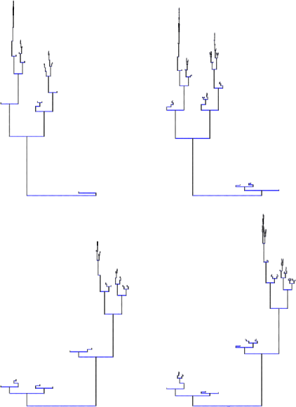
Figure 1: The metric tree for the odd (upper part) and even (lower part) $\pi$-data, for $n=50$ (left) and $n=100$ (right), respectively; see text for details.

The subtree size metric also leads to a visualization of search trees: We use the function $\beta$ defined in (2) to map nodes to points in the unit interval, and above the $x$-coordinate $\beta(u)$ we draw a line parallel to the $y$-axis from $d_{X_{n}}(\bar{u},\varnothing)$ to $d_{X_{n}}(u,\varnothing)$. In order to obtain a visually more pleasing result we may add lines that run parallel to the $x$-axis, connecting nodes with the same parent. In Figure 1 we have carried this out for the trees arising from two separate input sequences for the BST algorithm, with the data obtained from alternating blocks of length 10 of digits in the decimal expansion of $\pi-3$. The upper part refers to the odd and the lower to the even numbered blocks. In both cases we have given the trees for $n=50$ and $n=100$, and with $\rho=1$. Vertically, the trees are from the same distribution; moving horizontally to the right, we have almost sure convergence.

4 Tree functionals

In this section we show how the above results can be used in connection with the asymptotic analysis of tree functionals. Here is the recipe: We start with a functional $Y_{n}=\Psi_{n}(X_{n})$ of the trees, with (deterministic) functions $\Psi_{n}$ on $\mathbb{B}_{n}$ that have values in some separable Banach space $(\mathbb{L},\|\cdot\|)$. We suspect that $Y_{n}$ converges almost surely to some limit variable $Y_{\infty}$ as $n\to\infty$. We know that if this is the case, then $Y_{\infty}=\Psi(X_{\infty})$ for some $\Psi$ defined on $\partial\mathbb{B}$ (as always, almost surely). We do not know what $\Psi$ is, but if we manage to rewrite the $\Psi_{n}$’s in terms of subtree sizes, then Theorem 1 may lead to an educated guess. On that basis we next consider $\Phi_{n}(X_{n})=E[\Psi(X_{\infty})|\mathcal{F}_{n}]$, assuming that $E\|\Psi(X_{\infty})\|<\infty$. This gives an $\mathbb{L}$-valued martingale. By the associated convergence theorem we then have that $\tilde{Y}_{n}:=\Phi_{n}(X_{n})$ converges to $Y_{\infty}$ almost surely and in mean. Finally, a simple inspection of $\Phi_{n}-\Psi_{n}$ may reveal that $\tilde{Y}_{n}-Y_{n}$ is asymptotically negligible—indeed, if $Y_{n}$ converges to $Y_{\infty}$, then $\tilde{Y}_{n}-Y_{n}$ must tend to 0.

In the first three subsections we work out the details of the above strategy for path lengths, for a tree index and for an infinite dimensional tree functional. The final subsection is a collection of remarks on other functionals and related tree structures, indicating further applications of the method, but also its limitations. The potential-theoretic approach can provide additional insight; for example, we will relate a martingale introduced in connection with tree profiles to Doob’s $h$-transform.

Throughout this section we abbreviate $X_{\infty}(A_{u})$ to $X_{\infty}(u)$.

4.1 Path length

The first tree functional we consider is the internal path length,

$$\operatorname{IPL}(x):=\sum_{u\in x}|u|,\qquad x\in\mathbb{B},$$ (26)

which may be rewritten as

$$\operatorname{IPL}(x)=\sum_{u\in x,u\neq\varnothing}\sigma(x,u)=\sum_{u\in x}\sigma(x,u)-\#x.$$ (27)

Let

$$H(0):=0,\qquad H(n):=\sum_{i=1}^{n}\frac{1}{i}\qquad\mbox{for all }n\in\mathbb{N},$$

be the harmonic numbers. It is well known that

$$\lim_{n\to\infty}\bigl{(}H(n)-\log n\bigr{)}=\gamma,$$

where $\gamma\approx 0.57722$ is Euler’s constant. We need two auxiliary statements; we omit the (easy) proofs.

Lemma 4

For all $i,j\in\mathbb{N}_{0}$,

$$\frac{\Gamma(i+j+2)}{\Gamma(i+1)\Gamma(j+1)}\int_{0}^{1}x^{i}(1-x)^{j}\log(x)\,dx=H(i)-H(i+j+1).$$

For a random variable $\eta$ with distribution $\operatorname{Beta}(i+1,j+1)$ Lemma 4 leads to

$$E\bigl{(}\eta\log(\eta)\bigr{)}=\frac{i+1}{i+j+2}\bigl{(}H(i+1)-H(i+j+2)\bigr{)}.$$ (28)

The next lemma is a summation by parts formula for binary trees.

Lemma 5

For any function $\psi:\mathbb{V}\to\mathbb{R}$,

$$\sum_{u\in x}\bigl{(}\psi(u)-\psi(u0)-\psi(u1)\bigr{)}=\psi(\varnothing)-\sum_{u\in\partial x}\psi(u)\qquad\mbox{for all }x\in\mathbb{B}.$$

Major parts of the following theorem are known; we will give details later in order to be able to refer to the proof for a comparison of the methods used. Let $(X_{n})_{n\in\mathbb{N}}$ be the BST chain, and let $X_{\infty}$ be its limit, as in Theorem 3.

Theorem 6

Let $C\dvtx(0,1)\to\mathbb{R}$ be defined by

$$C(s):=1+2\bigl{(}s\log(s)+(1-s)\log(1-s)\bigr{)}.\vspace*{-9pt}$$

[(a)]

The limit

$$Y_{\infty}:=\sum_{u\in\mathbb{V}}X_{\infty}(u)C\biggl{(}\frac{X_{\infty}(u0)}{X_{\infty}(u)}\biggr{)}$$

exists almost surely and in quadratic mean.

As $n\to\infty$,

$$\frac{1}{n}\operatorname{IPL}(X_{n})-2\log n\to 2\gamma-4+Y_{\infty},$$ (29)

almost surely and in quadratic mean.

From the representation of $X_{\infty}$ given in Section 2.3, we know that the random variables

$$\xi_{u}:=\frac{X_{\infty}(u0)}{X_{\infty}(u)},\qquad u\in\mathbb{V},$$

are independent and uniformly distributed on the unit interval, and that $X_{\infty}(u)$ is a function of the $\xi_{v}$’s with $v<u$. In particular, for all nodes $u$, the two factors in the sum appearing in the definition of $Y_{\infty}$ are independent. Let $\mathcal{G}_{k}$ be the $\sigma$-field generated by the $\xi_{u}$’s with $|u|\leq k$, and put

$$Y_{k}:=\sum_{u\in\mathbb{V},|u|\leq k}X_{\infty}(u)C\biggl{(}\frac{X_{\infty}(u0)}{X_{\infty}(u)}\biggr{)},\qquad k\in\mathbb{N}.$$

Then these properties lead to

$$E[Y_{k+1}|\mathcal{G}_{k}] = Y_{k}+E\biggl{[}\sum_{|u|=k+1}X_{\infty}(u)C\biggl{(}\frac{X_{\infty}(u0)}{X_{\infty}(u)}\biggr{)}\Big{|}\mathcal{G}_{k}\biggr{]}$$

$$= Y_{k}+\sum_{|u|=k+1}X_{\infty}(u)EC(\xi_{u})$$

$$= Y_{k},$$

where we have used the fact that $EC(\xi_{u})=0$. Further, with the same arguments,

$$E\bigl{[}(Y_{k+1}-Y_{k})^{2}|\mathcal{G}_{k}\bigr{]} = E\biggl{[}\biggl{(}\sum_{|u|=k+1}X_{\infty}(u)C(\xi_{u})\biggr{)}^{2}\Big{|}\mathcal{G}_{k}\biggr{]}$$

$$= \sum_{|u|=k+1}X_{\infty}(u)^{2}EC(\xi_{u})^{2},$$

so that

$$E(Y_{k+1}-Y_{k})^{2}=\sum_{|u|=k+1}EX_{\infty}(u)^{2}EC(\xi_{u})^{2}.$$

We also have $\kappa:=EC(\xi_{u})^{2}<\infty$, and using (2.3) we get

$$EX_{\infty}(u)^{2}=\bigl{(}E\xi_{\varnothing}^{2}\bigr{)}^{k}=3^{-k},$$

so that

$$E(Y_{k+1}-Y_{k})^{2}=2^{k}3^{-k}\kappa\qquad\mbox{for all }k\in\mathbb{N}.$$ (30)

Taken together these calculations show that $(Y_{k},\mathcal{G}_{k})_{k\in\mathbb{N}}$ is an $L^{2}$-bounded martingale, and an appeal to the corresponding martingale limit theorem completes the proof of (a). In particular, $Y_{\infty}$ is well defined, and even has finite second moment.

For the proof of (b) let $Z_{n}:=E[Y_{\infty}|\mathcal{F}_{n}]$, $n\in\mathbb{N}$, so that $(Z_{n},\mathcal{F}_{n})_{n\in\mathbb{N}}$ is again a martingale bounded in $L^{2}$. Our plan is to show that $Z_{n}$ is sufficiently close to the transformed internal path length that appears in (29).

Using again the stochastic structure of $X_{\infty}$ we are thus led to consider the conditional expectations $E[X_{\infty}(u)|\mathcal{F}_{n}]$ and $E[C(\xi_{u})|\mathcal{F}_{n}]$, $u\in\mathbb{V}$ and $n\in\mathbb{N}$. From Proposition 2 we know that, for all $u\in X_{n}$,

$$\mathcal{L}(\xi_{u}|\mathcal{F}_{n})=\operatorname{Beta}\bigl{(}\sigma(X_{n},u0)+1,\sigma(X_{n},u1)+1\bigr{)},$$

and that the $\xi_{u}$’s are conditionally independent given $\mathcal{F}_{n}$. Hence Lemma 4 can be applied [see also (28)], resulting in

$$E\bigl{[}C(\xi_{u})|\mathcal{F}_{n}\bigr{]} = 1+\frac{2\tau(X_{n},u0)+2\tau(X_{n},u1)}{\sigma(X_{n},u0)+\sigma(X_{n},u1)+2}$$

$${}-2H\bigl{(}\sigma(X_{n},u0)+\sigma(X_{n},u1)+2\bigr{)},$$

where the function $\tau:\mathbb{B}\times\mathbb{V}\to\mathbb{R}$ is given by

$$\tau(x,u):=\bigl{(}\sigma(x,u)+1\bigr{)}H\bigl{(}\sigma(x,u)+1\bigr{)}.$$

For each fixed $n\in\mathbb{N}$, almost sure convergence of $E[Y_{k}|\mathcal{F}_{n}]$ to $E[Y_{\infty}|\mathcal{F}_{n}]$ as $k\to\infty$ follows from

$$\bigl{\|}E[Y_{k}|\mathcal{F}_{n}]-E[Y_{\infty}|\mathcal{F}_{n}]\bigr{\|}_{2}\leq\|Y_{k}-Y_{\infty}\|_{2},$$

the upper bound in (30) and the Borel–Cantelli lemma. Together with the conditional independence of $X_{\infty}(u)$ and $C(\xi_{u})$ given $\mathcal{F}_{n}$, this leads to

$$Z_{n}=\sum_{u\in\mathbb{V}}E\bigl{[}X_{\infty}(u)|\mathcal{F}_{n}\bigr{]}E\bigl{[}C(\xi_{u})|\mathcal{F}_{n}\bigr{]}.$$ (32)

From (4.1) we obtain $E[C(\xi_{u})|\mathcal{F}_{n}]=0$ for $u\notin X_{n}$, and, clearly,

$$\sigma(X_{n},u0)+\sigma(X_{n},u1)+1=\sigma(X_{n},u)\qquad\mbox{for all }u\in X_{n}.$$ (33)

Taken together, (25), (4.1), (32) and (33) lead to

$$Z_{n}=\sum_{u\in X_{n}}\frac{\sigma(X_{n},u)+1}{n+1}\biggl{(}1+\frac{2\tau(X_{n},u0)+2\tau(X_{n},u1)}{\sigma(X_{n},u)+1}-2H\bigl{(}\sigma(X_{n},u)+1\bigr{)}\biggr{)},$$

which in turn gives

$$Z_{n}=\frac{1}{n+1}\bigl{(}\operatorname{IPL}(X_{n})+2n\bigr{)}-\frac{2}{n+1}\sum_{u\in X_{n}}\bigl{(}\tau(X_{n},u)-\tau(X_{n},u0)-\tau(X_{n},u1)\bigr{)}.$$

Lemma 5 can be applied to the second sum, and the assertion finally follows from $\tau(X_{n},\varnothing)=(n+1)H(n+1)$ and $\tau(X_{n},u)=1$ for $u\in\partial X_{n}$.

Almost sure convergence of the standardized internal path length for the BST sequence has been obtained in RegnierQS , and convergence in distribution, together with a fixed point relation for the limit distribution, in RoeQS . Our method may been seen as an amalgamation of Régnier’s martingale approach and Rösler’s approach, where the latter has come to be known as the contraction method in the analysis of algorithms: We obtain a strong limit, but we do not need to “find the martingale” (a task familiar to many an applied probabilist). The approach suggested in the present paper, to look at convergence of the full objects via a suitable completion of the state space of the underlying combinatorial Markov chain, leads to a representation of the almost sure limit. This gives the martingale by projection via conditional expectations, and from the representation one can also read off a fixed point relation for the distribution of the limit.

4.2 The Wiener index

The canonical graph distance $d_{\mathrm{can}}(u,v)$ of any two nodes $u$ and $v$ in a finite connected graph $G$ with node set $V$ is the minimum length of a path (sequence of edges) that connects $u$ and $v$ in $G$. The sum of these distances is the Wiener index of the graph,

$$\operatorname{WI}(G):=\frac{1}{2}\sum_{(u,v)\in V\times V}d_{\mathrm{can}}(u,v),$$ (34)

introduced by the chemist H. Wiener. Some background together with pointers to the literature is given in Nein02 , which is also our main reference in this subsection. Among other results it is shown in Nein02 that for the BST sequence $(X_{n})_{n\in\mathbb{N}}$ the rescaled Wiener indices,

$$W_{n}:=\frac{1}{n^{2}}\operatorname{WI}(X_{n})-2\log n,$$

converge in distribution as $n\to\infty$.

Again, we project a suitable functional $\Psi(X_{\infty})$ of the limit tree $X_{\infty}$ to a function $E[\Psi(X_{\infty})|\mathcal{F}_{n}]$ of $X_{n}$ that is sufficiently close to $W_{n}$. This will give a strong limit theorem, that is, it turns out that the rescaled Wiener indices in fact converge almost surely for the random binary trees generated by the BST algorithm for i.i.d. input, and it will also lead to a representation of the limit $W_{\infty}$ as a function of $X_{\infty}$.

We begin by rewriting the Wiener index in terms of subtree sizes, similar to the transition from (26) to (27) in the analysis of the internal path length. For a binary tree $x$,

$$\sum_{(u,v)\in x\times x}|u\wedge v|=\sum_{u\in x}\sigma(x,u)^{2}.$$ (35)

This may be proved by induction, using the left and right subtrees in the induction step; see DennDiss , page 70. Using (16), (27), (34) and (35) we now obtain

$$\operatorname{WI}(X_{n})=n\operatorname{IPL}(X_{n})+n^{2}-\sum_{u\in X_{n}}\sigma(X_{n},u)^{2}.$$ (36)

It is a benefit of working with almost sure convergence that we can deal with the constituents on the right-hand side of (36) separately (which means that we can make use of Theorem 6), whereas in connection with convergence in distribution one needs to consider the joint distribution of $\operatorname{IPL}(X_{n})$ and $\operatorname{WI}(X_{n})$; see Nein02 .

Theorem 7

The series

$$Z_{\infty}:=\sum_{u\in\mathbb{V}}X_{\infty}(u)^{2}$$ (37)

converges almost surely and in quadratic mean, and, as $n\to\infty$,

$$\frac{1}{n^{2}}\operatorname{WI}(X_{n})-2\log n\to W_{\infty}$$ (38)

again almost surely and in quadratic mean, where the limit is given by

$$W_{\infty}:=2\gamma-3+Y_{\infty}-Z_{\infty},$$ (39)

with $Y_{\infty}$ as in Theorem 6.

Almost sure convergence in (37) follows with Theorem 3, and the moment calculations below show that $EZ_{\infty}^{2}<\infty$. In particular,

$$Z_{n}:=E[Z_{\infty}|\mathcal{F}_{n}]\to Z_{\infty}$$

almost surely and in quadratic mean. Again, the Markov property implies that $Z_{n}$ can be written as a function of $X_{n}$. In order to obtain this function we first consider a fixed node $u\in\mathbb{V}$.

From (2.3) we get

$$X_{\infty}(u)^{2}=\prod_{j=0}^{k-1}\tilde{\xi}_{u(j)}^{2}.$$

From (15) and the known formula for the second moment of beta distributions we obtain, considering the cases $u(j+1)=u(j)0$ and $u(j+1)=u(j)1$ separately,

$$E\bigl{[}\tilde{\xi}_{u(j)}^{2}|\mathcal{F}_{n}\bigr{]}$$

$$\qquad=\frac{(\sigma(X_{n},u(j+1))+1)(\sigma(X_{n},u(j+1))+2)}{(\sigma(X_{n},u(j)0)+\sigma(X_{n},u(j)1)+2)(\sigma(X_{n},u(j)0)+\sigma(X_{n},u(j)1)+3)}.$$

Using the conditional independence statement in Proposition 2, we see that we have a telescoping product again, so that

$$E\bigl{[}X_{\infty}(u)^{2}|\mathcal{F}_{n}\bigr{]}=\frac{(\sigma(X_{n},u)+1)(\sigma(X_{n},u)+2)}{(n+1)(n+2)}\qquad\mbox{for all }u\in X_{n}\cup\partial X_{n}.$$

The set $\mathbb{V}\setminus X_{n}$ can be written as the disjoint union of the subtrees rooted at the $n+1$ external nodes of $X_{n}$, and we have

$$E\bigl{[}\xi_{u}^{2}|\mathcal{F}_{n}\bigr{]}=E\bigl{[}(1-\xi_{u})^{2}|\mathcal{F}_{n}\bigr{]}=\tfrac{1}{3}\qquad\mbox{for all }u\notin X_{n}.$$

Therefore,

$$\sum_{u\notin X_{n}}E\bigl{[}X_{\infty}(u)^{2}|\mathcal{F}_{n}\bigr{]}$$

$$\qquad=\frac{1}{(n+1)(n+2)}\sum_{u\in\partial X_{n}}\bigl{(}\sigma(X_{n},u)+1\bigr{)}\bigl{(}\sigma(X_{n},u)+2\bigr{)}\sum_{v\in\mathbb{V},v\geq u}\biggl{(}\frac{1}{3}\biggr{)}^{|v|-|u|}$$

$$\qquad=\frac{2}{(n+1)(n+2)}\sum_{u\in\partial X_{n}}\sum_{k=0}^{\infty}2^{k}\biggl{(}\frac{1}{3}\biggr{)}^{k}$$

$$\qquad=\frac{6}{n+2}$$

in view of $\sigma(X_{n},u)=0$ for $u\in\partial X_{n}$. Taken together this gives

$$Z_{n}=\frac{1}{(n+1)(n+2)}\sum_{u\in X_{n}}\bigl{(}\sigma(X_{n},u)+1\bigr{)}\bigl{(}\sigma(X_{n},u)+2\bigr{)}+\frac{6}{n+2}.$$

Using (27) we get

$$\sum_{u\in X_{n}}\bigl{(}\sigma(X_{n},u)+1\bigr{)}\bigl{(}\sigma(X_{n},u)+2\bigr{)}=\sum_{u\in X_{n}}\sigma(X_{n},u)^{2}+3\cdot\operatorname{IPL}(X_{n})+5n$$

so that, with (36),

$$\frac{1}{(n+1)(n+2)}\operatorname{WI}(X_{n})=\frac{n}{(n+1)(n+2)}\operatorname{IPL}(X_{n})+\frac{n^{2}}{(n+1)(n+2)}-Z_{n}+R_{n},$$

where $R_{n}$ tends to 0 almost surely and in quadratic mean. From Theorem 6 we know that

$$\frac{1}{n}\operatorname{IPL}(X_{n})-2\log n\to 2\gamma-4+Y_{\infty}$$

in the same sense. Combining the last two statements we obtain (38), with $W_{\infty}$ as in (39).

4.3 Metric silhouette

In our third application we consider an infinite-dimensional tree functional.

Each element $v=(v_{k})_{k\in\mathbb{N}}$ of $\partial\mathbb{V}$ defines a path through a binary tree via the sequence $(v(k))_{k\in\mathbb{N}}$ of nodes given by $v(k)=(v_{1},\ldots,v_{k})$, $k\in\mathbb{N}$. In GrSilh the “silhouette” $\operatorname{Sil}(x)$ of $x\in\mathbb{B}$ was introduced in an attempt to obtain a search tree analogue of the famous Harris encoding of simply generated trees: with each path $v$, we record its exit level when passing through $x$, that is,

$$\operatorname{Sil}(x)(v):=\min\bigl{\{}k\in\mathbb{N}:v(k)\notin x\bigr{\}},\qquad v\in\partial\mathbb{V}.$$

The tree silhouette can be visualized as a function on the unit interval via the binary expansion

$$\Phi\dvtx[0,1)\to\partial\mathbb{V},\qquad t\mapsto(v_{k})_{k\in\mathbb{N}}\qquad\mbox{with }v_{k}:=\bigl{\lceil}2^{k+1}t\bigr{\rceil}-2\bigl{\lceil}2^{k}t\bigr{\rceil}.$$ (40)

It was shown in GrSilh that for the BST chain $(X_{n})_{n\in\mathbb{N}}$ some smoothing is necessary to obtain an interesting limit for the stochastic processes$(\operatorname{Sil}(X_{n})(\Phi(t)))_{0\leq t<1}$ as $n\to\infty$.

We have seen in the previous sections that for search trees it makes sense to replace the canonical tree distance implicit in the above definition of $\operatorname{Sil}(x)$ by the subtree size metric. A corresponding variant of the silhouette is the metric silhouette,

$$\operatorname{mSil}(x)(v):=\sum_{k=1}^{\infty}\sigma\bigl{(}x,v(k)\bigr{)},\qquad v\in\partial\mathbb{V}.$$

Again, our aim is to obtain a strong limit theorem in the BST situation, together with a representation of the limit as a function of $X_{\infty}$. In addition, and going beyond the individual arguments $v\in\partial\mathbb{V}$, we regard $\operatorname{mSil}(X_{n})$ as a random function on $\partial\mathbb{V}$. With $d_{\mathbb{V}}$ as in (8) this is a compact and separable metric space ($\mathbb{V}$ is open in the completion $\bar{\mathbb{V}}$ that we introduced in Section 2.3). We write $C(\partial\mathbb{V},d_{\mathbb{V}})$ for the space of continuous functions $f\dvtx\partial\mathbb{V}\to\mathbb{R}$. Together with

$$\|f\|_{\infty}:=\sup_{v\in\partial\mathbb{V}}\bigl{|}f(v)\bigr{|},$$

this is a separable Banach space.

Remember that the values of $X_{\infty}$ are probability measures on $(\partial\mathbb{V},\mathcal{B}(\partial\mathbb{V}))$. Let $\Sigma_{\infty}:\partial\mathbb{V}\to[0,\infty]$ be defined by

$$\Sigma_{\infty}(v):=-\int_{\partial\mathbb{V}}\log_{2}\bigl{(}d_{\mathbb{V}}(u,v)\bigr{)}X_{\infty}(du),\qquad v\in\partial\mathbb{V}.$$

This is the logarithmic potential of the random measure $X_{\infty}$ with respect to $d_{\mathbb{V}}$; see Woess1 , page 62. Finally, we recall that a real function $f$ on the metric space $(\partial\mathbb{V},d_{\mathbb{V}})$ is said to be (globally) Hölder continuous with exponent $\alpha$ if there exists a constant $C<\infty$ such that

$$\bigl{|}f(u)-f(v)\bigr{|}\leq Cd_{\mathbb{V}}(u,v)^{\alpha}\qquad\mbox{for all }u,v\in\partial\mathbb{V}.$$

Theorem 8

Let $\alpha_{0}:=\log_{2}\rho_{0}=0.33464\ldots$ with $\rho_{0}$ as in Theorem 3. [(a)]

$E\|\Sigma_{\infty}\|_{\infty}<\infty$.

With probability 1, $\Sigma_{\infty}$ is Hölder continuous with exponent $\alpha$ for all $\alpha<\alpha_{0}$.

As $n\to\infty$,

$$\biggl{\|}\frac{1}{n}\operatorname{mSil}(X_{n})-\Sigma_{\infty}\biggr{\|}_{\infty}\to 0\qquad\mbox{almost surely and in mean}.$$

Because of $d_{\mathbb{V}}(u,v)=2^{-|u\wedge v|}$ for all $u,v\in\partial\mathbb{V}$ we have$-\log_{2}d_{\mathbb{V}}(u,v)\in\mathbb{N}_{0}$ and

$$-\log_{2}d_{\mathbb{V}}(u,v)\geq k\quad\Longleftrightarrow\quad u\in A_{v(k)}$$

for all $k\in\mathbb{N}$ so that

$$\Sigma_{\infty}(v)=\sum_{k=1}^{\infty}X_{\infty}\bigl{(}v(k)\bigr{)}\qquad\mbox{for all }v\in\partial\mathbb{V}.$$ (41)

Now let $\alpha$ be as in the statement of the theorem; we may assume that $\alpha>0$. Let $\rho:=2^{\alpha}$. By Theorem 3 there exists a set of probability 1 such that for all $\omega$ in this set, $C(\omega):=\|X_{\infty}(\omega)\|_{\rho}<\infty$. We fix such an $\omega$ and drop it from the notation. Because of $X_{\infty}(u)\leq C\rho^{|u|}$ for all $u\in\mathbb{V}$ and (41), we then have $\Sigma_{\infty}(v)\leq C\sum_{k=1}^{\infty}\rho^{-k}$ for all $v\in\partial\mathbb{V}$, which implies

$$\|\Sigma_{\infty}\|_{\infty}\leq\frac{1}{\rho-1}\|X_{\infty}\|_{\rho}.$$

In particular, $E\|\Sigma_{\infty}\|_{\infty}<\infty$ by (19) in the proof of Theorem 3.

Similarly, if $u,v\in\partial\mathbb{V}$ are such that $|u\wedge v|=k$, then

$$\bigl{|}\Sigma_{\infty}(u)-\Sigma_{\infty}(v)\bigr{|} = \sum_{j=k+1}^{\infty}X_{\infty}\bigl{(}u(j)\bigr{)}+\sum_{j=k+1}^{\infty}X_{\infty}\bigl{(}v(j)\bigr{)}$$

$$\leq 2C\sum_{j=k+1}^{\infty}\rho^{-j}=\frac{2C\rho^{-k}}{\rho-1}\leq\frac{2C}{\rho-1}d_{\mathbb{V}}(u,v)^{\alpha}$$

by definition of $\rho$. This proves (b).

For the proof of (c) we first consider the random functions $\Sigma_{n}$ defined by

$$\Sigma_{n}(v):=E\bigl{[}\Sigma_{\infty}(v)|\mathcal{F}_{n}\bigr{]},\qquad v\in\partial\mathbb{V}.$$

With $J:=\operatorname{Sil}(X_{n})(v)$ we get, using monotone convergence for conditional expectations and $\mathcal{F}_{n}$-measurability of $J$,

$$\Sigma_{n}(v) = \sum_{k=1}^{J}E\bigl{[}X_{\infty}\bigl{(}v(k)\bigr{)}|\mathcal{F}_{n}\bigr{]}+\sum_{k=J+1}^{\infty}E\bigl{[}X_{\infty}\bigl{(}v(k)\bigr{)}|\mathcal{F}_{n}\bigr{]}$$

$$= \sum_{k=1}^{J}\frac{\sigma(X_{n},v(k))+1}{n+1}+\frac{\sigma(X_{n},v(J))+1}{n+1}\sum_{k=J+1}^{\infty}\biggl{(}\frac{1}{2}\biggr{)}^{k-J}$$

$$= \frac{1}{n+1}\bigl{(}\operatorname{mSil}(X_{n})(v)+J\bigr{)}+\frac{1}{n+1}.$$

Here we have used our formula (25) for $E[\Sigma_{\infty}(u)|\mathcal{F}_{n}]$ and its extension to nodes outside $X_{n}$ that can be obtained as in the proof of Theorem 7.

Let $h(x)=\max\{|u|:u\in x\}$ be the height of $x\in\mathbb{B}$. Taking the supremum over $v\in\partial\mathbb{V}$ we get

$$\biggl{\|}\Sigma_{n}-\frac{1}{n+1}\operatorname{mSil}(X_{n})\biggr{\|}_{\infty}\leq\frac{h(X_{n})+1}{n+1}.$$

It is easy to show that the right-hand side converges to 0 with probability 1 (see Dev86 for techniques and results on the height), so it remains to prove that $\Sigma_{n}$ converges almost surely and in mean to $\Sigma_{\infty}$ in the separable Banach space $(C(\partial\mathbb{V},d_{\mathbb{V}}),\|\cdot\|_{\infty})$. This, however, is again immediate from the vector-valued martingale convergence theorem given in NeveuMart , page 104.

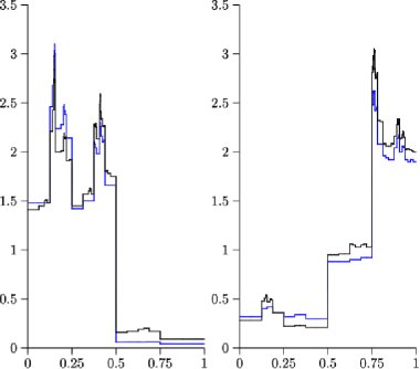
Figure 2: The metric silhouette for the odd (left) and even (right) $\pi$-data, with $n=50$ (blue) and $n=100$ (black).

Figure 2 shows the metric silhouette for the trees in Figure 1. Note that the continuity in Theorem 8 refers to the space $(\partial\mathbb{V},d_{\mathbb{V}})$; for example, $(t_{n})_{n\in\mathbb{N}}$ with $t_{n}=\frac{1}{2}+(-1)^{n}\frac{1}{n}$ for all $n\in\mathbb{N}$ is a Cauchy sequence with respect to euclidean distance, but its inverse under the function $\Phi$ defined in (40) that we used for the illustration is not a Cauchy sequence in $(\partial\mathbb{V},d_{\mathbb{V}})$. Loosely speaking, the function $\beta$ “flattens” the node set $\mathbb{V}$.

4.4 Other functionals and tree structures

The fill (or saturation) level $F(x)$ and height $H(x)$ of a tree $x\in\mathbb{B}$ are defined by

$$F(x)=\max\bigl{\{}k\in\mathbb{N}_{0}\dvtx\{0,1\}^{k}\subset x\bigr{\}},\qquad H(x)=\max\bigl{\{}|u|:u\in x\bigr{\}},$$

respectively. For these tree functionals, the following asymptotic results are well known:

$$\frac{F(X_{n})}{\log n}\to\alpha_{-},\qquad\frac{H(X_{n})}{\log n}\to\alpha_{+}\qquad\mbox{as }n\to\infty,$$ (42)

both almost surely. Here $\alpha_{-}=0.373\ldots$ and $\alpha_{+}=4.311\ldots$ are the two solutions of the equation $x\log(2e/x)=1$. The survey DevGelbesBuch gives details and references, and explains the relation to branching processes.

In situations such as these, where the almost sure limit is a constant, projection on the sub-$\sigma$-fields $\mathcal{F}_{n}$ would simply return the constant, hence no simplification arises.

Both the fill level and height of a tree as well as its path length (see Section 4.1) can be written as functionals of the tree’s node profile. Recall that $|u|$ denotes the length of $u\in\mathbb{V}$. Let

$$v(x,k):=\#\bigl{\{}u\in\partial x\dvtx|u|=k\bigr{\}},\qquad w(x,k):=\#\bigl{\{}u\in x\dvtx|u|=k\bigr{\}}$$

be the number of external (resp., internal) nodes of $x\in\mathbb{B}$ at depth $k$. Applied to the BST sequence $(X_{n})_{n\in\mathbb{N}}$, this gives sequences $(V_{n})_{n\in\mathbb{N}}$ and $(W_{n})_{n\in\mathbb{N}}$ of random functions on the nonnegative integers via $V_{n}(k)=v(X_{n},k)$ and $W_{n}(k)=w(X_{n},k)$, the external and internal node profile of the binary search tree. Clearly,

$$F(X_{n}) = \min\bigl{\{}k\in\mathbb{N}:V_{n}(k)>0\bigr{\}}-1,$$

$$H(X_{n}) = \max\bigl{\{}k\in\mathbb{N}:W_{n}(k)>0\bigr{\}}$$

and

$$\operatorname{IPL}(X_{n})=\sum_{k=1}^{\infty}kW_{n}(k),$$

so such profiles go some way toward a unifying approach to tree functionals and indeed, they have been studied extensively; see J-H2001 , CDJ2001 , CR2004 , CKMR2005 , FHN2006 , DJN2008 . A crucial role in J-H2001 , CDJ2001 , CR2004 , CKMR2005 is played by a parametrized family of martingales introduced in J-H2001 . In order to connect this to the point of view of the present paper we rephrase the basic idea using our terminology and notation.

Fix some $z\in\mathbb{R}_{+}$. The external profile $V_{n}$ of $X_{n}$ can be regarded as the counting density of a random finite measure on $\mathbb{N}$ with total mass $n+1$ and value

$$Y_{n}:=\sum_{k=1}^{\infty}V_{n}(k)z^{k}=\sum_{u\in\partial X_{n}}z^{|u|}$$

at $z$ of its generating function. Let $v$ be the random node that is added to $X_{n}$ to obtain $X_{n+1}$. It is easy to see that

$$Y_{n+1}=Y_{n}+z^{|v|}(2z-1).$$

In the BST mechanism the node $v$ is chosen uniformly at random from the $n+1$ external nodes of $X_{n}$, hence

$$E[Y_{n+1}|\mathcal{F}_{n}] = E\biggl{[}\sum_{v\in\partial X_{n}}\bigl{(}Y_{n}+z^{|v|}(2z-1)\bigr{)}1_{\{X_{n+1}=X_{n}\cup\{v\}\}}\Big{|}\mathcal{F}_{n}\biggr{]}$$

$$= Y_{n}E\biggl{[}\sum_{v\in\partial X_{n}}1_{\{X_{n+1}=X_{n}\cup\{v\}\}}\Big{|}\mathcal{F}_{n}\biggr{]}$$

$${}+(2z-1)E\biggl{[}\sum_{v\in\partial X_{n}}z^{|v|}1_{\{X_{n+1}=X_{n}\cup\{v\}\}}\Big{|}\mathcal{F}_{n}\biggr{]}$$

$$= Y_{n}+\frac{2z-1}{n+1}\sum_{v\in\partial X_{n}}z^{|v|}$$

$$= \frac{n+2z}{n+1}Y_{n},$$

which means that $(M_{n},\mathcal{F}_{n})_{n\in\mathbb{N}}$ with

$$M_{n}:=C(n)Y_{n},\qquad C(n):=\prod_{k=1}^{n-1}\frac{k+1}{k+2z}\mbox{ for all }n\in\mathbb{N},$$

is a martingale. Obviously, the martingale is strictly positive whenever $z>0$. Because of the space–time property it can therefore be written as $M_{n}=h(X_{n})$ with some positive harmonic function $h$ on $\mathbb{B}$, which depends on $z>0$, and which in the present context is given by

$$h(x)=C(\#x)\sum_{u\in\partial x}z^{|u|}.$$

Moreover, the distribution $P^{h}$ of the corresponding $h$-transform, which is the Markov chain with transition probabilities

$$p^{h}(x,y)=\frac{1}{h(x)}p(x,y)h(y),\qquad x,y\in\mathbb{B},$$

is such that for all $n\in\mathbb{N}$ the restriction $P^{h}_{\mathcal{F}_{n}}$ of $P^{h}$ to $\mathcal{F}_{n}$ has density

$$\frac{dP^{h}_{\mathcal{F}_{n}}}{dP_{\mathcal{F}_{n}}}=\frac{1}{2z}h(X_{n})$$

with respect to the restriction $P_{\mathcal{F}_{n}}$ to $\mathcal{F}_{n}$ of the distribution $P$ of the original BST chain. Here we have used that both chains start with the tree $X_{1}=\{\varnothing\}$, and that $h(\{\varnothing\})=2z$. A straightforward calculation yields

$$p^{h}\bigl{(}x,x\cup\{v\}\bigr{)}=\frac{1}{n+2z}\frac{\sum_{u\in\partial x}z^{|u|}+z^{|v|}(2z-1)}{\sum_{u\in\partial x}z^{|u|}}$$ (43)

for all $x\in\mathbb{B}$, $v\in\partial x$. Note that this agrees with the transition mechanism of the BST chain if $z=1/2$ or $z=1$. For general $z>0$ a corresponding chain may be constructed by a marking mechanism that makes use of an additional spine variable. This idea was introduced in the context of branching processes; for search trees it has been used in CKMR2005 , to which paper we refer for more details. The following direct construction of a Markov chain with transitions as in (43) may be of interest: Given $X_{n}$, we choose an external node $u$ with probability proportional to $z^{|u|}$. With probability $(2z)/(n+2z)$ we then accept $u$ as the node $v$ to be added to $X_{n}$; if $u$ is rejected, then $v$ is chosen uniformly at random from the other $n$ external nodes of $X_{n}$.

In the first three subsections of the present section we began our analysis by relating the functionals in question to the subtree sizes. As the latter fully describe the tree this must also be possible in the profile context. For $x\in\mathbb{B}$, $z>0$ let

$$\Psi_{z}(x):=\sum_{u\in x}\sigma(x,u)z^{|u|}.$$

Each $v\in\mathbb{V}_{k+1}$ with $\bar{v}\in x$ is either an internal or an external node of $x$, which means that $v(x,k+1)=2w(x,k)-w(x,k+1)$. Also, the number of internal nodes with depth at least $k$ is the sum of all subtree sizes of the nodes with level exactly equal to $k$, that is, $\sum_{u\in x,|u|=k}\sigma(x,u)=\sum_{j=k}^{\infty}w(x,j)$. Taken together, this gives

$$\sum_{k=1}^{\infty}v(x,k)z^{k}=\biggl{(}2z-3+\frac{1}{z}\biggr{)}\Psi_{z}(x)+\biggl{(}2-\frac{1}{z}\biggr{)}\#x+1,$$

which leads to

$$Y_{n}=\biggl{(}2z-3+\frac{1}{z}\biggr{)}\Psi_{z}(X_{n})+\biggl{(}2-\frac{1}{z}\biggr{)}n+1$$

(note that the bracketed term vanishes for $z=1/2$ and $z=1$). This could serve as the basis for an analysis along the lines of the first three subsections. We do not pursue this here but show instead that the general theory can be used to obtain an interpretation of the function that represents the limit of Jabbour’s martingale in terms of the Doob–Martin limit of the BST sequence: Recall that $M_{n}/(2z)$ is the density associated with the change of measure from $P_{\mathcal{F}_{n}}$ to $P^{h}_{\mathcal{F}_{n}}$. If the convergence $M_{n}\to M_{\infty}$ is in $L^{1}$ (see below), then $M_{\infty}/(2z)$ is a density of $P^{h}$ with respect to $P$. Thus we have $M_{\infty}=2z\Psi(X_{\infty})$, with $\Psi$ a density of the distribution of $X_{\infty}$ under the transformed measure $P^{h}$ with respect to the distribution of $X_{\infty}$ under the original $P$.

It is shown in CKMR2005 that $L^{1}$-convergence holds if and only if the parameter $z$ is inside a specific bounded interval $I=(c_{-},c_{+})$, that $M_{\infty}\equiv 0$ if $z\notin I$, and that, with $\alpha_{+},\alpha_{-}$ as in (42), $c_{-}=\alpha_{-}/2$ and $c_{+}=\alpha_{+}/2$. These two phase transitions are related to the asymptotics of the maximum and minimum node size respectively at a specific level of the limit $X_{\infty}$: If $z$ is too small, then nodes close to the root are favored too much by $p^{h}$; if $z$ is too large, then too much weight is given to nodes far away from the root. In both cases $P^{h}$ is then singular with respect to $P$. For the weighted subtree size metric considered in Section 3 only one of these caveats matters in that node sizes must not be inflated too much. Hence there is only one such phase transition, which should be related to the height constant, and indeed, a straightforward calculation shows that $\rho_{0}=(2e)/\alpha_{+}$.

Finally, let us mention that the approach toward strong asymptotics of dynamic data structures that we have developed in detail for binary search trees should be applicable in many related situations. The necessary modifications may be minor, such as for the discounted path length that appears in GrSilh , or straightforward, as for the random recursive trees that are often treated in parallel with binary trees (see, e.g., Nein02 for the Wiener index), or they may be challenging, for example, when we wish to amplify the weak convergence results for node depth profiles obtained in DJN2008 for a wide class of trees to strong limit theorems as we have done for the Wiener index in Section 4.2. Of course, convergence in distribution and convergence along paths are rather different phenomena; see Figures 1 and 2. It is interesting that for a given dynamical structure we may have a strong limit theorem (with nontrivial limit) for some aspects (functionals), but not for others; see DeGr3 for such results in connection with the subtree size profile of binary search trees.

References

• (1) {barticle}[mr] \bauthor\bsnmBiggins, \bfnmJ. D.\binitsJ. D. (\byear1977). \btitleChernoff’s theorem in the branching random walk. \bjournalJ. Appl. Probab. \bvolume14 \bpages630–636. \bidissn=0021-9002, mr=0464415 \bptokimsref \endbibitem
• (2) {bbook}[mr] \bauthor\bsnmBillingsley, \bfnmPatrick\binitsP. (\byear1968). \btitleConvergence of Probability Measures. \bpublisherWiley, \blocationNew York. \bidmr=0233396 \bptokimsref \endbibitem
• (3) {barticle}[mr] \bauthor\bsnmBlackwell, \bfnmDavid\binitsD. and \bauthor\bsnmKendall, \bfnmDavid\binitsD. (\byear1964). \btitleThe Martin boundary of Pólya’s urn scheme, and an application to stochastic population growth. \bjournalJ. Appl. Probab. \bvolume1 \bpages284–296. \bidissn=0021-9002, mr=0176518 \bptokimsref \endbibitem
• (4) {bbook}[mr] \bauthor\bsnmBurago, \bfnmDmitri\binitsD., \bauthor\bsnmBurago, \bfnmYuri\binitsY. and \bauthor\bsnmIvanov, \bfnmSergei\binitsS. (\byear2001). \btitleA Course in Metric Geometry. \bseriesGraduate Studies in Mathematics \bvolume33. \bpublisherAmer. Math. Soc., \blocationProvidence, RI. \bidmr=1835418 \bptokimsref \endbibitem
• (5) {barticle}[mr] \bauthor\bsnmChauvin, \bfnmBrigitte\binitsB., \bauthor\bsnmDrmota, \bfnmMichael\binitsM. and \bauthor\bsnmJabbour-Hattab, \bfnmJean\binitsJ. (\byear2001). \btitleThe profile of binary search trees. \bjournalAnn. Appl. Probab. \bvolume11 \bpages1042–1062. \biddoi=10.1214/aoap/1015345394, issn=1050-5164, mr=1878289 \bptokimsref \endbibitem
• (6) {barticle}[mr] \bauthor\bsnmChauvin, \bfnmB.\binitsB., \bauthor\bsnmKlein, \bfnmT.\binitsT., \bauthor\bsnmMarckert, \bfnmJ. F.\binitsJ. F. and \bauthor\bsnmRouault, \bfnmA.\binitsA. (\byear2005). \btitleMartingales and profile of binary search trees. \bjournalElectron. J. Probab. \bvolume10 \bpages420–435 (electronic). \biddoi=10.1214/EJP.v10-257, issn=1083-6489, mr=2147314 \bptokimsref \endbibitem
• (7) {barticle}[auto:STB—2013/10/14—10:36:11] \bauthor\bsnmChauvin, \bfnmBrigitte\binitsB. and \bauthor\bsnmRouault, \bfnmAlain\binitsA. (\byear2004). \btitleConnecting Yule processes, bisection and binary search tree via martingales. \bjournalJ. Iran. Stat. Soc. (JIRSS) \bvolume3 \bpages89–116. \bptokimsref \endbibitem
• (8) {bmisc}[auto:STB—2013/10/14—10:36:11] \bauthor\bsnmDennert, \bfnmFlorian\binitsF. (\byear2009). \bhowpublishedZufällige binäre Bäume: Algorithmen, Asymptotik und Statistik. Ph.D. thesis, Leibniz Univ. Hannover. \bptokimsref \endbibitem
• (9) {barticle}[mr] \bauthor\bsnmDennert, \bfnmFlorian\binitsF. and \bauthor\bsnmGrübel, \bfnmRudolf\binitsR. (\byear2010). \btitleOn the subtree size profile of binary search trees. \bjournalCombin. Probab. Comput. \bvolume19 \bpages561–578. \biddoi=10.1017/S0963548309990630, issn=0963-5483, mr=2647493 \bptokimsref \endbibitem
• (10) {barticle}[mr] \bauthor\bsnmDevroye, \bfnmLuc\binitsL. (\byear1986). \btitleA note on the height of binary search trees. \bjournalJ. Assoc. Comput. Mach. \bvolume33 \bpages489–498. \biddoi=10.1145/5925.5930, issn=0004-5411, mr=0849025 \bptokimsref \endbibitem
• (11) {bincollection}[mr] \bauthor\bsnmDevroye, \bfnmLuc\binitsL. (\byear1998). \btitleBranching processes and their applications in the analysis of tree structures and tree algorithms. In \bbooktitleProbabilistic Methods for Algorithmic Discrete Mathematics. \bseriesAlgorithms Combin. \bvolume16 \bpages249–314. \bpublisherSpringer, \blocationBerlin. \bidmr=1678582 \bptokimsref \endbibitem
• (12) {barticle}[mr] \bauthor\bsnmDoob, \bfnmJ. L.\binitsJ. L. (\byear1959). \btitleDiscrete potential theory and boundaries. \bjournalJ. Math. Mech. \bvolume8 \bpages433–458; erratum 993. \bidmr=0107098 \bptokimsref \endbibitem
• (13) {bbook}[mr] \bauthor\bsnmDrmota, \bfnmMichael\binitsM. (\byear2009). \btitleRandom Trees: An Interplay Between Combinatorics and Probability. \bpublisherSpringer, \blocationVienna. \biddoi=10.1007/978-3-211-75357-6, mr=2484382 \bptokimsref \endbibitem
• (14) {barticle}[mr] \bauthor\bsnmDrmota, \bfnmMichael\binitsM., \bauthor\bsnmJanson, \bfnmSvante\binitsS. and \bauthor\bsnmNeininger, \bfnmRalph\binitsR. (\byear2008). \btitleA functional limit theorem for the profile of search trees. \bjournalAnn. Appl. Probab. \bvolume18 \bpages288–333. \biddoi=10.1214/07-AAP457, issn=1050-5164, mr=2380900 \bptokimsref \endbibitem
• (15) {bbook}[mr] \bauthor\bsnmEvans, \bfnmSteven N.\binitsS. N. (\byear2008). \btitleProbability and Real Trees. \bseriesLecture Notes in Math. \bvolume1920. \bpublisherSpringer, \blocationBerlin. \biddoi=10.1007/978-3-540-74798-7, mr=2351587 \bptokimsref \endbibitem
• (16) {barticle}[mr] \bauthor\bsnmEvans, \bfnmSteven N.\binitsS. N., \bauthor\bsnmGrübel, \bfnmRudolf\binitsR. and \bauthor\bsnmWakolbinger, \bfnmAnton\binitsA. (\byear2012). \btitleTrickle-down processes and their boundaries. \bjournalElectron. J. Probab. \bvolume17 \bpages1–58. \biddoi=10.1214/EJP.v17-1698, issn=1083-6489, mr=2869248 \bptokimsref \endbibitem
• (17) {barticle}[mr] \bauthor\bsnmFuchs, \bfnmMichael\binitsM. (\byear2008). \btitleSubtree sizes in recursive trees and binary search trees: Berry–Esseen bounds and Poisson approximations. \bjournalCombin. Probab. Comput. \bvolume17 \bpages661–680. \biddoi=10.1017/S0963548308009243, issn=0963-5483, mr=2454562 \bptokimsref \endbibitem
• (18) {barticle}[mr] \bauthor\bsnmFuchs, \bfnmMichael\binitsM., \bauthor\bsnmHwang, \bfnmHsien-Kuei\binitsH.-K. and \bauthor\bsnmNeininger, \bfnmRalph\binitsR. (\byear2006). \btitleProfiles of random trees: Limit theorems for random recursive trees and binary search trees. \bjournalAlgorithmica \bvolume46 \bpages367–407. \biddoi=10.1007/s00453-006-0109-5, issn=0178-4617, mr=2291961 \bptokimsref \endbibitem
• (19) {barticle}[mr] \bauthor\bsnmGrübel, \bfnmRudolf\binitsR. (\byear2009). \btitleOn the silhouette of binary search trees. \bjournalAnn. Appl. Probab. \bvolume19 \bpages1781–1802. \biddoi=10.1214/08-AAP593, issn=1050-5164, mr=2569807 \bptokimsref \endbibitem
• (20) {barticle}[mr] \bauthor\bsnmJabbour-Hattab, \bfnmJean\binitsJ. (\byear2001). \btitleMartingales and large deviations for binary search trees. \bjournalRandom Structures Algorithms \bvolume19 \bpages112–127. \biddoi=10.1002/rsa.1023, issn=1042-9832, mr=1848787 \bptokimsref \endbibitem
• (21) {bbook}[mr] \bauthor\bsnmKallenberg, \bfnmOlav\binitsO. (\byear1997). \btitleFoundations of Modern Probability. \bpublisherSpringer, \blocationNew York. \bidmr=1464694 \bptokimsref \endbibitem
• (22) {barticle}[mr] \bauthor\bsnmKaĭmanovich, \bfnmV. A.\binitsV. A. and \bauthor\bsnmVershik, \bfnmA. M.\binitsA. M. (\byear1983). \btitleRandom walks on discrete groups: Boundary and entropy. \bjournalAnn. Probab. \bvolume11 \bpages457–490. \bidissn=0091-1798, mr=0704539 \bptokimsref \endbibitem
• (23) {bbook}[mr] \bauthor\bsnmKnuth, \bfnmDonald E.\binitsD. E. (\byear1973). \btitleThe Art of Computer Programming. Vol. 3: Sorting and Searching. \bpublisherAddison-Wesley, \blocationReading, MA. \bidmr=0445948 \bptokimsref \endbibitem
• (24) {bbook}[mr] \bauthor\bsnmMahmoud, \bfnmHosam M.\binitsH. M. (\byear1992). \btitleEvolution of Random Search Trees. \bpublisherWiley, \blocationNew York. \bidmr=1140708 \bptokimsref \endbibitem
• (25) {barticle}[mr] \bauthor\bsnmNeininger, \bfnmRalph\binitsR. (\byear2002). \btitleThe Wiener index of random trees. \bjournalCombin. Probab. Comput. \bvolume11 \bpages587–597. \biddoi=10.1017/S0963548302005321, issn=0963-5483, mr=1940122 \bptokimsref \endbibitem
• (26) {bbook}[mr] \bauthor\bsnmNeveu, \bfnmJ.\binitsJ. (\byear1975). \btitleDiscrete-Parameter Martingales, \beditionRevised ed. \bpublisherNorth-Holland, \blocationAmsterdam. \bidmr=0402915 \bptokimsref \endbibitem
• (27) {barticle}[mr] \bauthor\bsnmRégnier, \bfnmMireille\binitsM. (\byear1989). \btitleA limiting distribution for quicksort. \bjournalRAIRO Inform. Théor. Appl. \bvolume23 \bpages335–343. \bidissn=0988-3754, mr=1020478 \bptokimsref \endbibitem
• (28) {barticle}[mr] \bauthor\bsnmRösler, \bfnmUwe\binitsU. (\byear1991). \btitleA limit theorem for “Quicksort.” \bjournalRAIRO Inform. Théor. Appl. \bvolume25 \bpages85–100. \bidissn=0988-3754, mr=1104413 \bptokimsref \endbibitem
• (29) {bbook}[mr] \bauthor\bsnmWoess, \bfnmWolfgang\binitsW. (\byear2000). \btitleRandom Walks on Infinite Graphs and Groups. \bseriesCambridge Tracts in Mathematics \bvolume138. \bpublisherCambridge Univ. Press, \blocationCambridge. \biddoi=10.1017/CBO9780511470967, mr=1743100 \bptokimsref \endbibitem
• (30) {bbook}[mr] \bauthor\bsnmWoess, \bfnmWolfgang\binitsW. (\byear2009). \btitleDenumerable Markov Chains: Generating Functions, Boundary Theory, Random Walks on Trees. \bpublisherEMS, \blocationZürich. \biddoi=10.4171/071, mr=2548569 \bptokimsref \endbibitem