High redshift Fermi blazars observed by GROND and Swift

Abstract

We observed 5 $\gamma$–ray loud blazars at redshift greater than 2 with the X–Ray Telescope (XRT) and the UltraViolet and Optical Telescope (UVOT) onboard the Swift satellite, and the Gamma–Ray burst Optical Near–Infrared Detector (GROND) instrument. These observations were quasi simultaneous, usually within a few hours. For 4 of these blazars the near–IR to UV data show the presence of an accretion disc, and we could reliably estimate its accretion rate and black hole mass. One of them, PKS 1348+007, was found in an extraordinarily high IR–optical state, almost two orders of magnitude brighter than at the epoch of the Sloan Digital Sky Survey observations. For all the 5 quasars the physical parameters of the jet emitting zone, derived by applying a one–zone emission model, are similar to that found for the bulk of other $\gamma$–ray loud quasars. With our observations we have X–ray data for the full sample of blazars at $z>2$ present in the Fermi 2–yrs (2LAC) catalog. This allows to have a rather complete view of the spectral energy distribution of all high–redshift Fermi blazars, and to draw some conclusions about their properties, and especially about the relation between the accretion rate and the jet power.

1 Introduction

High redshift blazars are the most powerful persistent sources, and are usually connected with the most massive black holes (Ghisellini et al. 2009; 2010a; Volonteri et al. 2011). The Large Area Telescope (LAT) onboard the Fermi satellite (Atwood et al. 2009) and the Burst Alert Telescope (BAT) onboard Swift (Gehrels et al. 2004) have provided tens of detections of blazars at $z>2$ (Abdo et al. 2010, Ackermann et al. 2011; Ajello et al. 2009, Cusumano et al. 2010; Baumgartner et al. 2010). The combinations of the two sets of data (Swift+Fermi) have allowed to measure the properties and the bolometric luminosity of the jet non–thermal emission and to characterize the thermal component emitted by the accretion disc, namely the black hole mass $M$ and the accretion rate $\dot{M}$. It is found (Ghisellini et al. 2010b; 2011) that in powerful blazars black hole masses are usually greater than $10^{9}M_{\odot}$, with disc luminosities $L_{\rm d}\sim$0.1$L_{\rm Edd}$, jet kinetic powers $P_{\rm j}\sim\dot{M}c^{2}$, with $P_{\rm j}$ tightly related to $L_{\rm d}$. This can test jet production models, since $P_{\rm j}\lower 2.15277pt\hbox{$\;\buildrel>\over{\sim}\;$}\dot{M}c^{2}$ requires that we are using another source of energy besides accretion, namely we must extract the black hole spin energy (see e.g. Tchekhovskoy, Narayan & McKinney 2011).

In order to find the physical parameters of these sources it is very important to have a good coverage of their spectral energy distribution (SED), that allows us to constrain the model parameters. Moreover, blazars are varying fast (hours to days, especially at high frequencies), and with large amplitudes (even by factor 10 or more in the $\gamma$–ray range, but sometimes even in the optical) implying that simultaneous observations are needed to well constrain their SED.

High redshift blazars are interesting “per se”, since we would like to know if and how the jet properties change with cosmic time. High redshift also usually means larger luminosities and powers, and this allows to study the more powerful jets. If we define a blazar as a source whose jet is observed with a viewing angle $\theta_{\rm v}<1/\Gamma$ ($\Gamma$ is the bulk Lorentz factor), then there must be other $2\Gamma^{2}$ similar objects whose jet is pointing elsewhere and whose flux is dramatically fainter (because of beaming). These misaligned sources share all the intrinsic properties of the blazar that is pointing at us, including the black hole mass. If we are able to estimate it for a blazar, we can put very interesting constraints on the density of heavy black holes of all radio sources in the young Universe (see Volonteri et al. 2011).

From the $z>2$ blazars detected by Fermi/LAT, we have chosen those with no data in the X–ray range (or with only an upper limit), and have organized a simultaneous observational campaign involving the X–Ray Telescope (XRT) and the UltraViolet and Optical Telescope (UVOT) onboard Swift (Gehrels et al. 2004) and the Gamma–Ray burst Optical Near–Infrared Detector (GROND) instrument (Greiner et al. 2008). The scientific rationale for observing these blazars at X–ray and IR–optical frequencies is the following. In powerful blazars, the [0.3–10 keV] Swift band is where we expect the contribution of the inverse Compton emission of the jet. This is usually made by two components, according if the scattering process makes use of internally produced synchrotron seed photons (Synchrotron Self Compton, or SSC for short) or if the seeds are produced externally to the jet (External Compton, EC). They are usually characterized by a different spectrum and variability behavior, and the relative importance of the two gives information on the magnetic field and the bulk Lorentz factor. In the near IR, optical and UV bands, instead, we have the contributions of the accretion disc and the beamed synchrotron component. If we can distinguish the two contributions then we can estimate the black hole mass and the accretion rate (from the disc emission), and have information of the value of the magnetic field (from the synchrotron flux).

The starting samples were the Fermi/LAT detected blazars at $z>2$ present in the Fermi blazar catalogs after 11 months of operations (1LAC, Abdo et al. 2010) and after 2 years (2LAC, Ackermann et al. 2011). In the 1LAC catalog there are 2 sources observed by Swift in 2009 for just a ks, for which we could only derive an upper limit to the X–ray flux. In the 2LAC catalog there are 3 new blazars at $z>2$ (out of 31) without a proper characterization of their SED, because of no information on their X–ray flux, useful to characterize the jet beamed emission, nor good data coverage in the IR–optical–UV band, useful to derive the thermal (i.e. accretion disc) contribution. These 5 blazars are all at declination $<$+30^∘, and are visible from La Silla, where the GROND instrument operates. Therefore we organized quasi–simultaneous Swift and GROND observing campaigns for these blazars.

These observations provided us with optical–UV–X–ray information on the entire high redshift Fermi sample (“clean” 2LAC with $z>2$). Tab. 1 lists the 5 selected blazars, together with their $\gamma$–ray k–corrected luminosities. These are the averaged luminosity over 11 months (1LAC) and 2 yrs (2LAC). For the blazars 1149–084 and 1344–1723, present in both catalogs, we give the corresponding two luminosities.

With a good simultaneous coverage from the near IR to X–ray range, in addition to the Fermi data, we can properly characterize the SED in order to disentangle the non–thermal jet contribution and the thermal component, to find the black hole mass, the accretion rate, and the physical jet quantities (magnetic field, bulk Lorentz factor, particle densities and jet power).

We use a flat cosmology with $H_{0}=70$ km s^-1 Mpc^-1, $\Omega_{\rm M}$=0.3 and the notation $Q=10^{X}Q_{X}$ in cgs units.

Name	RA	Dec	$z$	$L_{\gamma,1}$	$L_{\gamma,2}$
PKS 0519+01	05 22 17.5	+01 13 31	2.941	…	47.0
TXS 1149–084	11 52 17.2	–08 41 03	2.367	47.7	47.7
MG2 J133305+2725	13 33 07.5	+27 25 18	2.126	…	47.3
PMN J1344–1723	13 44 14.4	–17 23 40	2.49	48.5	48.2
PKS 1348+007	13 51 04.4	+00 31 19	2.084	…	47.6

Table 1: List of our sources. $L_{\gamma,1}$ refers to the [0.1–10 GeV] $\gamma$–ray luminosity in the 1LAC catalog, while $L_{\gamma,2}$ is the one in the 2LAC catalog, in units of erg s^-1.

2 GROND observations and data analysis

The 7–band GROND imager is mounted at the 2.2 m MPG/ESO telescope at La Silla Observatory (Chile). GROND is able to observe simultaneously in 7 filters, from the NIR $Ks$ (2300 nm) to the $g^{\prime}$ band (360 nm). Therefore it nicely complements the UVOT filters, with the bluest ($g^{\prime}$ and $r^{\prime}$) filter overlapping in part with the reddest $v$ and $b$ UVOT filter (and this is useful for cross calibration).

We carried out observations for all sources simultaneously in all 7 $g^{\prime},r^{\prime},i^{\prime},z^{\prime},J,H,K_{\rm s}$ bands. The log of the GROND observations and the related observing conditions are reported in Tab. 2.

The GROND optical and NIR image reduction and photometry were performed using standard IRAF tasks (Tody 1993), similar to the procedure described in Krühler et al. (2008). A general model for the point–spread function (PSF) of each image was constructed using bright field stars, and it was then fitted to the point source. When the source field was covered by the SDSS (Smith et al. 2002) survey (i.e. PKS 0519+01, PKS 1348+007, MG2 J133305+2725), the absolute calibration of the $g^{\prime},r^{\prime},i^{\prime},z^{\prime}$ bands was obtained with respect to the magnitudes of SDSS stars within the blazar field. In the other cases (i.e. PMN J1344–1723 and TXS 1149–084), optical photometric calibration was performed relative to the magnitudes of six secondary standards in the blazar field. During photometric conditions, a primary SDSS standard field was observed within minutes of an observation of the source field. The obtained zero–points were corrected for atmospheric extinction and used to calibrate stars in the blazar field. The apparent magnitudes of the sources were measured with respect to these secondary standards. For all sources the $J,H,K_{\rm s}$ bands calibrations were obtained with respect to magnitudes of the Two Micron All Sky Survey (2MASS) stars (Skrutskie et al. 2006).

Tab. 3 reports the observed AB magnitudes, not corrected for the Galactic extinction listed in the last column and taken from Schlafly & Finkbeiner (2011).

3 Swift observations and data analysis

We have analysed the Swift X–Ray Telescope (XRT; Burrows et al. 2005) and Optical–Ultraviolet Telescope (UVOT; Roming et al. 2005) data. The data were screened, cleaned and analysed with the software package HEASOFT v. 6.12, with the calibration database updated to 22 March 2012. The XRT data were processed with the standard procedures (XRTPIPELINE v.0.12.6). All sources were observed in photon counting (PC) mode and grade 0–12 (single to quadruple pixel) were selected. The channels with energies below 0.3 keV and above 10 keV were excluded from the fit and the spectra were rebinned in energy so to have at least 20–30 counts per bin in order to apply the $\chi^{2}$ test. When there are no sufficient counts we applied the likelihood statistic in the form reported by Cash (1979). Each spectrum was analysed in XSPEC v. 12.7.1 with an absorbed power law model with a fixed Galactic column density as measured by Kalberla et al. (2005). The computed errors represent the 90% confidence interval on the spectral parameters. Tab. 4 reports the log of the observations and the best fit results of the X–ray data with a simple power law model. The X–ray spectra displayed in the SED have been rebinned to ensure the best visualization.

UVOT source counts were extracted from a circular region 5”–sized centred on the source position, while the background was extracted from an annulus with internal radius of 7” and variable outer radius depending on the nearest contaminating source. Data were integrated with the uvotimsum task and then analysed by using the uvotsource task. The observed magnitudes have been dereddened according to the formulae by Cardelli et al. (1989) and converted into fluxes by using standard formulae and zero points.

As can be seen, the UVOT observations yielded mostly upper limits, and very few detections. The listed UVOT and GROND magnitudes do not take into account any difference between the two instruments, that is however likely, and of the order of 0.1–0.3 magnitudes (see Rau et al. 2012), especially if the observations were not exactly simultaneous, but separated by a few hours (the maximum separation – two days – occurs for PKS 0519+01).

Name	Date	Start time	Exp: opt/IR	Average seeing	Average airmass
	yyyy–mm–dd	$[{\rm UTC}]$	[s]	[arcsec]
0519+01	2012–02–26	00:14:00	919/960	0.70	1.18
1149–084	2012–03–20	02:09:51	1501/1200	0.72	1.27
1333+2725	2012–05–09	02:40:11	426/720	1.31	1.83
1344–1723	2012–04–04	08:36:13	919/960	1.32	1.44
1348+007	2012–03–16	05:03:37	3002/2400	1.15	1.26
1348+007	2012–03–18	09:38:11	460/480	1.43	1.61

Table 2: Log of the GROND observations. Exposures refer to optical/NIR filters while the average seeing is calculated in the $r^{\prime}$ band.

Name	$g^{\prime}$	$r^{\prime}$	$i^{\prime}$	$z^{\prime}$	$J$	$H$	$K_{s}$	$A_{V}$
0519+01	20.37$\pm$0.05	19.83$\pm$0.05	19.50$\pm$0.05	19.28$\pm$0.05	18.74$\pm$0.11	18.54$\pm$0.11	18.61$\pm$0.15	0.38
1149–084	19.65$\pm$0.05	19.42$\pm$0.06	19.40$\pm$0.08	19.04$\pm$0.08	18.97$\pm$0.11	18.67$\pm$0.12	18.24$\pm$0.13	0.23
1333+2725	20.38$\pm$0.06	19.89$\pm$0.06	19.39$\pm$0.06	19.07$\pm$0.05	18.33$\pm$0.10	17.73$\pm$0.10	17.44$\pm$0.13	0.03
1344–1723	20.69$\pm$0.05	20.26$\pm$0.05	19.99$\pm$0.05	19.56$\pm$0.06	19.01$\pm$0.12	18.42$\pm$0.12	18.11$\pm$0.13	0.37
1348+007 (1)	19.65$\pm$0.05	19.25$\pm$0.05	18.90$\pm$0.05	18.62$\pm$0.06	18.25$\pm$0.10	17.79$\pm$0.10	17.40$\pm$0.12	0.11
1348+007 (2)	20.24$\pm$0.05	19.88$\pm$0.05	19.49$\pm$0.05	19.19$\pm$0.06	18.66$\pm$0.11	18.20$\pm$0.11	17.76$\pm$0.12	0.11

Table 3: Observed magnitudes, not corrected for Galactic foreground reddening, in the AB system. Errors include systematics. The last column reports the value of the Galactic $A_{V}$ from Schlafly & Finkbeiner (2011).

Name	Date	Exp.	$N^{\rm Gal}_{\rm H}$	$\Gamma$	$F_{X}$	$\chi^{2}$ (d.o.f.)	Note
	yyyy–mm–dd/UTC)	ks	cm-2		$10^{-13}$ cgs
0519+01	2012–02–24/01:26	21.9	1.07e21	1.76$\pm$0.24	3.1	76.28 (95)	Cash stat
1149–084	2012–03–19/00:10 $+$ 2012–03–20/08:09	17.1	4.75e20	1.49$\pm$0.28	2.5	70.02 (67)	Cash stat
1333+2725	2012–05–09/00:09 $+$ 2012–05–10/21:16	19.8	1.02e20	1.84$\pm$0.17	6.65	10.87 (12)
1344–1723	2012–04–03/10:55 $+$ 2012–04–04/01:41	14.9	8.70e20	1.87$\pm$0.40	1.5	36.68 (39)	Cash stat
1348+007	2012–03–16/04:51 $+$ 2012–03–18/13:17	17.5	2.22e20	1.50$\pm$0.26	2.9	82.27 (78)	Cash stat

Table 4: Observation log and results of the X–ray analysis of XRT data. The flux $F_{X}$ is in the [0.3–10 keV] band, it is de–absorbed with the indicated $N^{\rm Gal}_{\rm H}$ and it is in units of $10^{-13}$ erg cm^-2 s^-1. Apart from 0519+01, all other sources were observed in two occasions: the listed exposure time is the sum. The analysis has been performed on the total. All sources but 1333+2725 have been analyzed with the Cash statistics (Cash 1979; Gehrels 1986).

Name	$v$	$b$	$u$	$uvw1$	$uvm2$	$uvw2$
0519+01	$>$19.1	$>$20.0	$>$19.5	$>$19.6	$>$21.7	$>$21.9
1149–084	$>$19.1	$>$20.0	$>$19.7	$>$20.0	$>$20.6	$>$21.8
1333+2725	$>$19.2	$>$20.2	20.3$\pm$0.3	20.4$\pm$0.4	19.7$\pm$0.2	19.9$\pm$0.1
1344–1723	$>$19.0	$>$20.0	21.0$\pm$0.2	$>$19.9	$>$20.1	$>$20.7
1348+007	$>$19.1	$>$20.2	$>$20.8	$>$21.0	20.3$\pm$0.1	$>$20.8

Table 5: UVOT magnitudes. The magnitude lower limits are at the 3$\sigma$ level.

4 Spectral Energy Distributions and modelling

In Fig. 1–5 we show the spectral energy distribution (SED) of our sources. We complement our near–simultaneous data with archival data taken from NED and ASDC. We show the Fermi/LAT data of the 1LAC or 2LAC catalogs, but also the average flux corresponding to one month of Fermi observation, starting 2 weeks before and ending two weeks after the GROND+Swift observing time.

The adopted model is a one–zone and leptonic model, fully described in Ghisellini & Tavecchio (2009). The main properties are summarized in the Appendix, mainly to explain the meaning of the parameters listed in Tab. 6 and Tab. 7.

In brief, the model assumes that the bulk of the jet dissipation takes place in one zone located at some distance $R_{\rm diss}$ from the black hole. For simplicity, the emitting region is assumed spherical with a radius $R=\psi R_{\rm diss}$, with $\psi=0.1$. The region is moving with a bulk Lorentz factor $\Gamma$, and is observed under a viewing angle $\theta_{\rm v}$. Energetic electrons are injected throughout the source for a time equal to the light crossing time $R/c$, and the particle distribution is calculated (through the continuity equation) at this time, considering radiative losses and possible electron–positron pair production and their reprocessing. In the following we briefly discuss the guidelines for the choice of the main parameters needed for the model.

Name	$z$	$R_{\rm diss}$	$M$	$R_{\rm BLR}$	$P^{\prime}_{\rm i}$	$L_{\rm d}$	$B$	$\Gamma$	$\gamma_{\rm b}$	$\gamma_{\rm max}$	$s_{1}$	$s_{2}$
[1]	[2]	[3]	[4]	[5]	[6]	[7]	[8]	[9]	[10]	[11]	[12]	[13]
0519+01	2.941	540 (400)	4.5e9	486	0.011	23.6 (0.035)	1.9	11	50	3e3	1	2.5
1149–084	2.367	180 (400)	1.5e9	561	0.01	31.5 (0.14)	7.9	15	300	800	–1	3.3
		720 (600)	4e9	849	0.015	72 (0.12)	1.39	14	300	3e3	–1	2
1333+2725	2.126	45 (1500)	1e8	300	0.01	9 (0.6)	5.5	13	600	1.8e3	0	2.4
1344–1723	2.49	225 (500)	1.5e9	351	0.021	12.3 (0.055)	2.3	13	1.4e3	2.3e3	0	2.7
		330 (1100)	1e9	274	0.027	7.5 (0.05)	0.89	13	1.4e3	8e3	–1	2.5
1348 high	2.084	60 (500)	4e8	115	8.5e–3	1.3 (0.022)	4.5	11	500	4.7e3	–1	2.2
1348 low	2.084	96 (800)	4e8	115	2.2e–3	1.3 (0.022)	1.3	15	300	3e3	–1	2.5

Table 6: List of parameters used to construct the theoretical SED. Not all of them are “input parameters” for the model: $R_{\rm BLR}$ is uniquely determined from $L_{\rm d}$, and the cooling energy $\gamma_{\rm c}$ and $U^{\prime}$ are derived parameters. Col. [1]: name; Col. [2]: redshift; Col. [3]: dissipation radius in units of $10^{15}$ cm and (in parenthesis) in units of Schwarzschild radii; Col. [4]: black hole mass in solar masses; Col. [5]: size of the BLR in units of $10^{15}$ cm; Col. [6]: power injected in the blob calculated in the comoving frame, in units of $10^{45}$ erg s^-1; Col. [7]: accretion disc luminosity in units of $10^{45}$ erg s^-1 and (in parenthesis) in units of $L_{\rm Edd}$; Col. [8]: magnetic field in Gauss; Col. [9]: bulk Lorentz factor at $R_{\rm diss}$; Col. [10] and [11]: break and maximum random Lorentz factors of the injected electrons; Col. [12]: and [13]: slopes of the injected electron distribution [$Q(\gamma)$] below and above $\gamma_{\rm b}$; For all sources we assumed a viewing angle $\theta_{\rm v}=3^{\circ}$. The total X–ray corona luminosity is assumed to be in the range 10–30 per cent of $L_{\rm d}$. Its spectral shape is assumed to be always $\propto\nu^{-1}\exp(-h\nu/150~{}{\rm keV})$. The parameters in italics refer to the physical quantities found in Ghisellini et al. (2011).

4.1 Guidelines for the choice of the parameters

The luminosity of the accretion disc — It can be estimated directly if the disc is visible and its spectrum peaks in the observed frequency range. This occurs for PKS 0519+01, for TXS 1149–084 and most likely for PMN J1344–1723, even if in this latter blazar there is a strong “contaminating” synchrotron component. The overall luminosity $L_{\rm d}$ of a standard accretion disc is roughly twice its $\nu L(\nu)$ peak, therefore we can directly estimate $L_{\rm d}$ if we see a thermal peak in the SED. For MG2 J1333+2725 the IR to UV continuum is dominated by the steep tail of the synchrotron flux, while in PKS 1348+007 we have a hint of the contribution from the accretion disc from the photometric data of the SDSS. If an optical spectrum is available (as in the case of TXS 1149–084 and PMN J1344–1723, Shaw et al. 2012), we have additional information from the luminosity of the broad emission lines. Through the templates of Francis et al. (1991) and/or of Vanden Berk et al (2001) we can reconstruct, from the luminosity of one or more lines, the entire luminosity of the broad line region, $L_{\rm BLR}$. Then, applying a typical covering factor $C$ (namely, $C\sim 0.1$), we can estimate $L_{\rm d}$. Finally, if no spectrum is available and the thermal component is completely swamped by the synchrotron flux, we can have a (rough) indication of $L_{\rm BLR}$ through the correlation between $L_{\rm BLR}$ and $L_{\gamma}$ as found by Sbarrato et al. (2012a). This has the form

$$L_{\rm BLR}\sim 4L_{\gamma}^{0.93}$$ (1)

Note, however, that since $L_{\gamma}$ can vary even by two orders of magnitude in the same source, the correlation necessarily has a large scatter, making the estimate of $L_{\rm BLR}$ (and thus of $L_{\rm d}$) uncertain.

Black hole mass — If $L_{\rm d}$ is determined reliably, there is only one black hole mass value that can fit the flux produced by (a standard) accretion disc. In this case the derived mass is robust, with an associated uncertainty of less than a factor 2 (see Fig. 1 in Sbarrato et al. 2012b, §4.4 and Fig. 1 below). If $L_{\rm d}$ is uncertain, this reflects also on the uncertainty on the derived black hole mass.

Location of the emitting region — One of the specific features of the model is that it calculates the energy densities (magnetic and radiative) as a function of the distance $R_{\rm diss}$ from the black hole. In particular, if $R_{\rm diss}<R_{\rm BLR}$, the energy density of the line photons as seen in the comoving frame becomes (up to a factor of order unity):

$$U^{\prime}_{\rm BLR}\,\sim\,\Gamma^{2}{L_{\rm BLR}\over 4\pi R^{2}_{\rm BLR}c}\,=\,{\Gamma^{2}\over 12\pi}$$ (2)

where we have used $R_{\rm BLR}\sim 10^{17}L^{1/2}_{\rm d,45}$ cm, and $C=0.1$. A similar relation holds for the IR radiation reprocessed by the torus located at a distance $R_{\rm IR}$, namely when $R_{\rm BLR}<R_{\rm diss}<R_{\rm IR}$. This limits $R_{\rm diss}$.

Magnetic field — The magnetic energy density, although is formally a free parameter, must satisfy the Compton to synchrotron luminosity ratio, i.e. $L_{\rm C}/L_{\rm syn}=U^{\prime}_{\rm rad}/U^{\prime}_{B}$. $U^{\prime}_{\rm rad}$ includes both internally produced radiation (i.e. by synchrotron) and radiation produced externally (directly by the disc or reprocessed and re–isotropized by the BLR and the torus).

Bulk Lorentz factor — The value of $\Gamma$ determines the value of the radiation energy density of the external seed photons ($\propto\Gamma^{2}$) and hence the value of the magnetic field required to have the observed synchrotron to inverse Compton luminosity ratio. Further information come from the peak frequencies of the synchrotron and inverse Compton components, that depend also on the break energy of the electron distribution.

Injected power — The power is injected throughout the source in the form of relativistic electrons. Through the continuity equation we calculate the particle distribution as a result of injection, cooling and possible pair production. The total injected power is such that the radiation produced by these particles agrees with the observed data. The injected distribution is assumed to be a smoothly broken power law (see Eq. 3 in the Appendix). The resulting distribution, modified by cooling, must agree with the observed slopes.

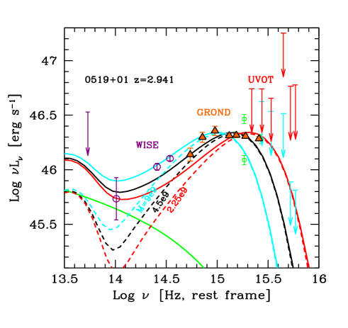
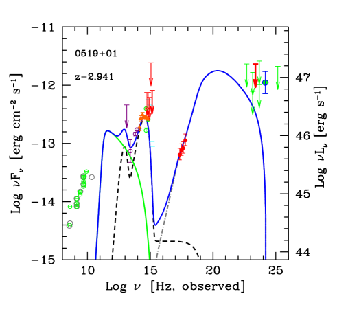
Figure 1: Top panel: a zoom of the SED of the blazar PKS 0519+01 in the IR, optical and UV. Light (cyan) arrows are the upper limit as observed by UVOT, darker (red) arrows are the same data de–absorbed by the predicted amount of Ly$\alpha$ forest absorption along the line of sight (see Ghisellini et al. 2010a). Triangles (orange) are the GROND data, empty circles are the WISE data. We also show three accretion disc models (short dashed lines) with the same accretion luminosity and three different black hole mass, from 2.25 to 9 billion solar masses (as labelled), together with the contribution of the torus emission, emitting in the IR. The thin solid (green) line is the synchrotron component, and the solid (cyan, black and red) lines are the sum of the accretion disc+torus+synchrotron flux. Note that WISE data are not simultaneous. Bottom: The entire SED of the PKS 0519+01, together with the adopted model. Filled (red) circles are the XRT data, and the (heavy) arrow in the $\gamma$–ray band is the upper limit corresponding to 1 month of Fermi data centered to the Swift+GROND observations, while the other arrows in the $\gamma$–ray band correspond to data from 2yr integration. Note also the detection at $\nu\sim 10^{24}$ Hz. Archival data are form the online service of ASI Science Data Center (ASDC, green filled circles) and NED (empty circles). Short dashed line: contribution from the accretion disc (with a black hole mass $M=4.5\times 10^{9}M_{\odot}$), IR torus and corona. Thin solid (green) line: synchrotron; dot–dashed line: EC component. Solid (blue) line: sum of all components.

4.2 Caveats

Within the framework of the adopted model, there is some degeneracy between a few set of parameters, that can be broken if some additional information, besides the SED, is provided. For instance, the bulk Lorentz factor and the viewing angle, together with the injected power in relativistic particles, can have a range of possible values. If, in addition, we have a limit on the variability timescale and/or the superluminal speed, then we can chose a unique set of parameters.

The black hole mass found by fitting a Shakura–Sunjaev disc to the near IR–optical–UV data gives excellent results if the flux at these frequencies is not contaminated by the synchrotron flux. Otherwise, the disc luminosity can be estimated rather accurately from the observed broad line luminosities, but the black hole mass can have a large uncertainty, partly mitigated by assuming that the disc cannot be super–Eddington (thus yielding a lower limit to the black hole mass).

Also the derived jet powers bear some uncertainties due to several unknowns: i) we do not know if charge neutrality is provided by protons, or by positrons. Recent studies (Ghisellini & Tavecchio 2010) have shown that a pure pair plasma would suffer a severe Compton drag while crossing the broad line region, limiting the positron/proton ratio to nearly 20 (in agreement with independent estimates put forward by Sikora & Madejski 2000); ii) we can estimate the amount of emitting particles, but there can be additional particles that are not accelerated, but nevertheless participate to the bulk motion of the jet, hence to its kinetic power; iii) the estimated magnetic field $B$ is the one in the emitting region. If the dissipation mechanism is magnetic reconnection, it is likely that in the emitting region $B$ is smaller than in the surroundings.

Bearing in mind these limitations, we now discuss the physical parameters found by adopting our model.

4.3 Physical parameters

Tab. 6 lists the parameters of the applied model. It also reports the parameters adopted in Ghisellini et al. (2011) for the two sources in common with that paper. Consider that the SED available at the time of Ghisellini et al. (2011) was largely incomplete, lacking the WISE, GROND and Swift data. Moreover, also the high frequency radio coverage has been improved with data provided by the Planck and WMAP satellites (see also Giommi et al. 2012 for a collection of blazar’s SED including Planck and WMAP data). The improved characterization of the SED of these blazars allowed a better estimate of the physical parameters: we find that although the values found now are not very different from what we have guessed before, the uncertainty is much less.

In general, all the derived parameters are well within the distributions derived for a large sample of $\gamma$–ray loud blazars studied in Ghisellini et al. (2010a). For all 5 blazars in our sample, the region dissipating most of the flux we see is located at several hundreds of Schwarzschild radii from the black hole, with bulk Lorentz factors in the range 10–15, and small viewing angle ($\theta_{\rm v}\sim 3^{\circ}$). The magnetic field is in the range 1–8 Gauss, and the intrinsic power injected in the form of relativistic electrons is of the order of $10^{44}$ erg s^-1, as measured in the comoving frame. The black hole mass is around $M\sim 10^{9}M_{\odot}$, with a luminosity of the accretion disc ranging from $10^{45}$ erg s^-1 (for PKS 1348+007) to $\sim$ (2–3)$\times 10^{46}$ erg s^-1 (for PKS 0519+01 and TXS 1149–084). These are all very typical values for FSRQs. In the following we discuss in more detail individual sources.

4.4 PKS 0519+01

Present in the 2LAC catalog, this $\gamma$–ray blazars had no previous X–ray information. There is no redshift in NED, the value for $z$ comes from the value listed in the 2LAC catalog, but the spectrum is still unpublished. Our observations (and the WISE data) greatly improve our knowledge of the SED, as shown in Fig. 1, despite the fact that for this source, the UVOT data were only upper limits. Note that for each UVOT upper limit we plot two arrows, corresponding to the observed datum and the de–absorbed one. The latter is derived assuming, along the line of sight, an average distribution of absorbing Ly$\alpha$ clouds (see Fig. 3 in Ghisellini et al. 2010a).

The GROND photometric points allow to determine the peak of the accretion disc spectrum, hence its luminosity $L_{\rm d}\sim 2\times 10^{46}$ erg s^-1 and black hole mass, that turns out to be $M=4.5\times 10^{9}M\odot$. This is the largest value we find for the 5 blazars here considered. To estimate the uncertainty for this value, we show in Fig. 1 the fit with a black hole mass of 2.25, 4.5 and 9 billion solar masses, as labelled, keeping the same $L_{\rm d}$. The fit with the largest mass underestimates the high frequency GROND point, while the fit with the lowest mass underestimates all but the high frequency GROND fluxes. We can conclude that the mass determination has an uncertainty, in this case, of less than a factor 2.

The bottom panel of Fig. 1 shows the complete SED of the source together with the model. We show, separately, the synchrotron component (solid light green line) the torus+disc+X–ray corona contribution (black short–dashed line) and the inverse Compton contribution, dominated by scattering with emission line seed photons (grey dot–dashed line). The thick (blue) solid line is the sum. We show also the Fermi upper limit on the $\gamma$–ray flux resulting from a month of data centered on the time of the Swift and GROND observations (thick red arrow).

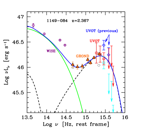
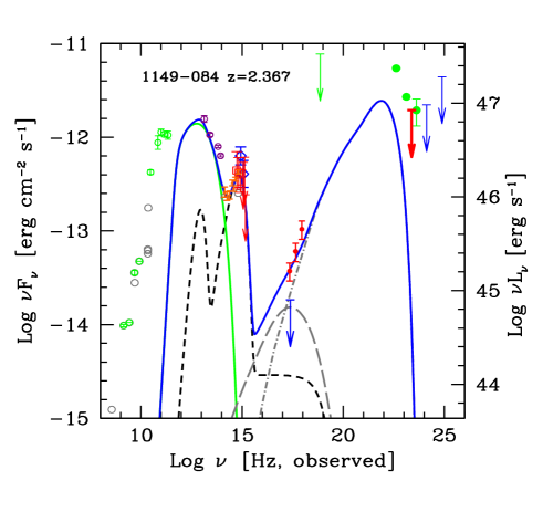
Figure 2: Lines and symbols as in Fig. 1, for TXS 1149–084. Bottom panel: in this case the SSC component (long dashed grey line) contributes to the soft X–ray flux. The upper limit in X–rays (blue arrow) corresponds to an earlier and very short (1 ks) Swift observation, when the source was detected in two UVOT filters as labelled in the top panel [“UVOT (previous)”].

4.5 TXS 1149–084

This source has been observed spectroscopically in the optical by Shaw et al. (2012), that reported a luminosity ($L_{\rm CIV}=2\times 10^{44}$ erg s^-1) and a FWHM (7200 km s^-1) of the CIV broad emission line, together with the luminosity of the continuum at 1350 Å ($L_{1350}=1.3\times 10^{46}$erg s^-1). These data allowed Shaw et al. (2012) to estimate a black hole mass of $M=2.4\times 10^{9}M_{\odot}$, applying the virial method. Using the template of Francis et al. (1991) and Vanden Berk (2001), one can derive the overall luminosity of the BLR, $L_{\rm BLR}\sim 2\times 10^{45}$ erg s^-1 and then a disc luminosity ten times greater (assuming a covering factor equal to 0.1). This value agrees well with the GROND+Swift data, from which we determined the peak of the disc component, with $L_{\rm d}=3.2\times 10^{46}$ erg s^-1. Therefore also in this case the black hole mass is well determined, $M=1.5\times 10^{9}M_{\odot}$.

In this source the WISE data, together with the high frequency radio data (from Planck) show a strong synchrotron component, peaking in the submm range. This is also indicated by the GROND data, showing un upturn towards the low frequencies. This upturn constrains the possible models capable of reproducing the synchrotron peak. The self–absorption frequency of our compact emitting zone occurs at $\sim$ 760 GHz (observed frame), making the synchrotron component very narrow. We derive a rather large magnetic field ($\sim$8 G), to account for the strength of the synchrotron flux. Accordingly, also the synchrotron Self Compton flux is not negligible, and contributes to the soft X–rays (long dashed grey curve in Fig. 2).

Also for this source we show the Fermi/LAT upper limit measured from 1–month of data around the time of the Swift and GROND observations.

Tab. 6 lists also the parameters used in Ghisellini et al. (2011), for which no GROND data were available and there was only an upper limit to the X–ray flux (shown as a blue arrow in Fig. 2), implying that the source has brightened in the X–ray band. The main differences with those results concern the black hole mass (it was $\sim$3 times greater), the value of $R_{\rm diss}$ (4 times larger) and the magnetic field (5.5 times smaller). The previous UVOT fluxes were slightly larger, and in the absence of additional optical IR data these resulted in an overestimation of the black hole mass and and disc luminosity (see Tab. 6), instead of a larger synchrotron flux. This well illustrates the importance of having a good coverage in the IR–optical, and also some information on the emission lines (from Shaw et al. 2012). The better coverage in the near and far IR and in the submm range allows to characterize better the synchrotron component, while the detection in the X–rays (at a flux larger than the previous upper limit) allows to determine the importance of the inverse Compton process (sum of SSC and EC). We find that the overall SED can be explained assuming a relatively strong synchrotron (and SSC) components, consequence of a magnetic field larger than the one assumed in Ghisellini et al. (2011).

Name	$\log P_{\rm r}$	$\log P_{\rm B}$	$\log P_{\rm e}$	$\log P_{\rm p}$	$\log P_{\rm j,min}$
0519+01	45.00	45.68	44.53	46.94	45.30
1149–084	45.08	46.22	43.93	46.16	45.38
	45.47	45.87	43.83	46.24	45.77
1333+2725	45.18	44.58	44.33	45.96	45.48
1344–1723	45.54	45.23	44.07	46.12	45.84
	45.66	44.74	44.43	46.03	45.96
1348 high	45.00	44.52	43.96	45.38	45.30
1348 low	44.68	44.12	43.59	45.34	44.98

Table 7: Logarithm of the jet power in the form of radiation ($P_{\rm r}$), Poynting flux ($P_{\rm B}$), bulk motion of electrons ($P_{\rm e}$) and protons ($P_{\rm p}$, assuming one proton per emitting electron). The last column lists the minimum jet power, calculated assuming that the radiation drag of the jet halves its bulk Lorentz factor. This limit corresponds to twice the radiated power $P_{\rm r}$. Powers are in erg s^-1. The parameters in italics refer to the physical quantities found in Ghisellini et al. (2011).

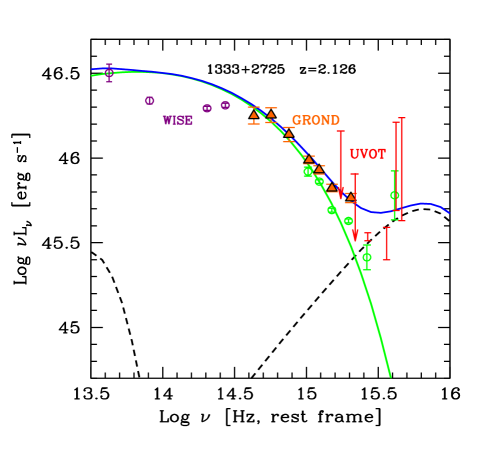
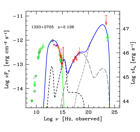
Figure 3: Lines and symbols as in Fig. 1, for MG2 J133305+2725. Also in this case, as for TXS 1149–084, the SSC component contributes to the soft X–ray flux. The bars in the bluest UVOT filters indicate the possible range of intrinsic flux levels: the lowest extremes correspond to the detected flux, and the highest extremes to the flux once de–absorbed by the average intervening Ly$\alpha$ absorption as calculated in Ghisellini et al. (2010).

4.6 MG2 J133305+2725

This is a blazar that is present in the photometric optical SDSS survey (with a magnitude $r=20.18$), but with no spectroscopic observations. UVOT detected the source in the bluest filters. At these frequencies the flux is partially absorbed by intervening Ly$\alpha$ clouds, whose total optical depth can be roughly calculated by averaging over many line of sights (as done in Ghisellini et al. 2010). There is however a large dispersion around these mean values, and for this reason we have indicated, with bars, the possible range of the de–absorbed UVOT fluxes.

The slope defined by the GROND data is steep, not consistent with a disc spectrum, that must therefore be hidden by the tail of the synchrotron flux. A strong synchrotron component is indeed needed by the WISE, WMAP and Planck data. However, for the fit, we have given less weight to the WISE data, since they are not simultaneous.

The emission disc component shown in Fig. 3 is only illustrative, but its luminosity cannot much be less than shown, due to the presence of the broad emission lines that make this blazar a FSRQs (but there is no published information on the line strength). For the black hole mass we have no strong constraints but a slight flattening of the GROND data towards the blue, possibly indicating an upturn of the spectrum. If due to the presence of the accretion disc, this implies a relatively small mass (i.e. a high maximum temperature), so we have chosen an illustrative value of $M=10^{8}M_{\odot}$. For this mass the disc must emit at 60% the Eddington rate.

A strong synchrotron component implies that the SSC flux can contribute to the soft X–ray spectrum, as shown in Fig. 3, while the EC component dominates the bolometric output as in the other sources.

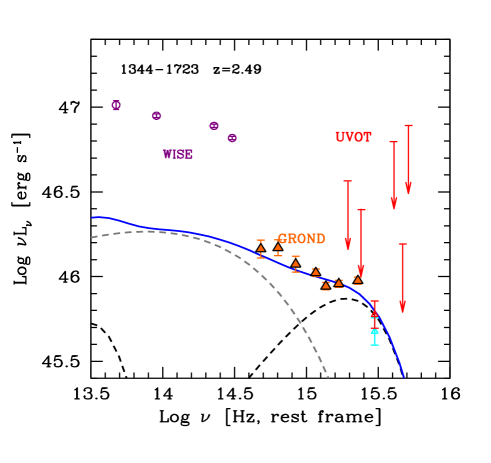
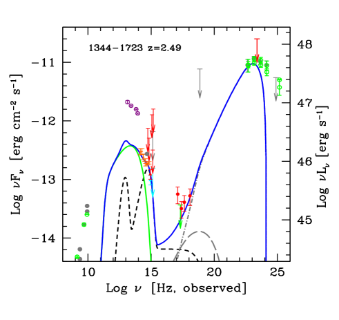
Figure 4: Lines and symbols as in Fig. 1, for PMN J1344–1723.

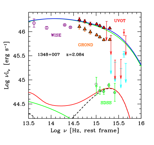
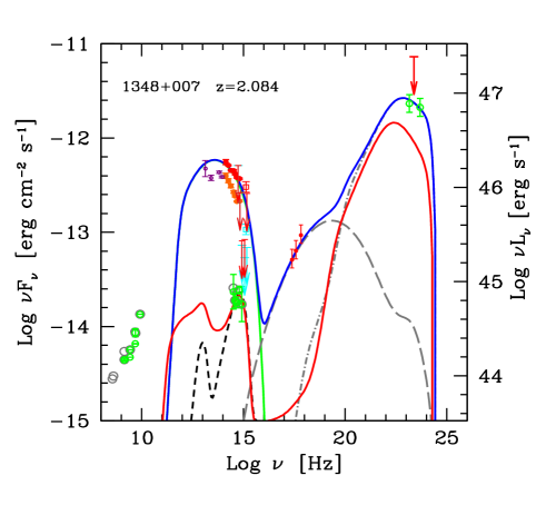
Figure 5: Lines and symbols as in Fig. 1, for PKS 1348+007. Note the large amplitude variability in the optical. The SDSS photometric fluxes, taken on May 20, 2009, are a factor $\sim$30 below the GROND+Swift+WISE data. Fast variability is present also in our GROND data, taken two nights apart (see Tab. 2, Tab. 3).

4.7 PMN J1344–1723

This source has been observed spectroscopically in the optical by Shaw et al. (2012), that derived the luminosity of the CIV broad line ($L_{\rm CIV}=10^{44}$ erg s^-1), corresponding (using Francis et al. 1991 or Vander Berk et al. 2001), to $L_{\rm BLR}\sim 10^{45}$ erg s^-1. Adopting a covering factor $C\sim 0.1$ we then have $L_{\rm d}\sim 10^{46}$ erg s^-1. The GROND data show a flattening (in $\nu F\nu$) of the spectrum, that we interpret as the emergence of the accretion disc component. With UVOT we have upper limits in all filters except in the $u$ band. Note that in $u$ the source is already affected by possible absorption by intervening Ly$\alpha$ clouds. In Fig. 4 both the observed and the de–absorbed flux are plotted. However, we caution about the large uncertainty connected with the use of an average distribution of absorbers along the line of sight. By decomposing the optical–UV emission with a synchrotron+accretion disc component, we derived $L_{\rm d}=1.2\times 10^{46}$ erg s^-1, in agreement with what is indicated by the CIV broad line. We then derive a black hole mass $M=1.5\times 10^{9}M_{\odot}$. This value is about the same as that derived by Shaw et al. (2012) using the virial method, the FWHM of the CIV broad line (6000 km s^-1) and the continuum luminosity at 1350 Å ($L_{1350}=5.9\times 10^{45}$erg s^-1), giving $M=1.3\times 10^{9}M_{\odot}$.

The WISE data indicate a strong synchrotron component. However, these data cannot connect smoothly with the GROND IR points, strongly suggesting that the synchrotron emission is variable with a large amplitude. This implies also that the blazar was in a somewhat low state at the epoch of our observations, and for this reason we did not attempt to accurately reproduce the $\gamma$–ray flux. For the model shown in Fig. 4 we have derived 2.3 Gauss for the magnetic field: with this value the SSC barely contributes to the soft X–rays. At higher X–ray energies the flux is completely dominated by the external Compton process (with line photons as seeds). The present set of data can be compared with what was known previously, and studied in Ghisellini et al. (2011, see their Fig. 5). One can appreciate the great improvement, and consequently the improved confidence on the derived physical quantities.

4.8 PKS 1348+007

This blazar showed an extraordinary optical flare, as derived by comparing the optical SDSS data ($r=22.4$) with our GROND and UVOT data, together with the IR flux seen by WISE. Fast variability is present also in our GROND data, taken two nights apart (see Tab. 2, Tab. 3 and Fig. 5). The source varied by about half a magnitude in all filters (except $K_{s}$), i.e. by $\sim$60% in flux. There is also a hint (although marginal) of a “harder when brighter” behaviour. Unfortunately, there are no SDSS spectra for this source. Comparing our data with the SDSS photometric data, obtained on May 20, 2009, the synchrotron emission had to vary by a factor $\sim$30. As can be seen in Fig. 5, the synchrotron component completely outshines the disc emission at the time of our GROND+Swift observations. Fortunately, the SDSS data hint to the presence of an accretion disc, through a flat (in $\nu F_{\nu}$) slope suggested by the photometric data. We have assumed that the SDSS fluxes are completely produced by the accretion disc, and derived a luminosity $L_{\rm d}=1.3\times 10^{45}$ erg s^-1 and a black hole mass $M=4\times 10^{8}M_{\odot}$.

The extraordinary optical variability of PKS 1348+007 is not unprecedented, being similar to the optical flare shown by 3C 454.3 in 2005 (Fuhrmann et al. 2006; Pian et al. 2006; Villata et al. 2006; Giommi et al., 2006). In principle, these large optical variations could be explained in two different scenarios. In the first, one can assume that the jet power is unchanged, but the dissipation regions varies and is smaller for the high optical state. The magnetic field, which should decrease along the jet, is larger for smaller $R_{\rm diss}$, implying a larger $U_{B}^{\prime}$. On the other hand, the radiation energy density of the broad line photons is constant within $R_{\rm BLR}$, and in the comoving frame is $U^{\prime}_{\rm BLR}\sim\Gamma^{2}/(12\pi)$ (see Eq. 2). Therefore the synchrotron to inverse Compton luminosity ratio $L_{\rm syn}/L_{\rm C}$ changes for varying $R_{\rm diss}$ even if the jet carries the same amount of power. In this case the $\gamma$–ray luminosity could remain constant or even decrease during an optical flare. Alternatively, the jet power can vary, making the optical and the $\gamma$–ray fluxes vary together. In this case an high optical state should be accompanied by a larger $\gamma$–ray flux.

Unfortunately, we do not have information about the high energy emission for the low optical state of the source, so we cannot distinguish between these two hypotheses. We have simply explored the first option, looking for a solution for both states that maintains the total jet power roughly constant. The two models shown in Fig. 5 correspond to the jet emission produced at $R_{\rm diss}=60$ and 96 Schwarzschild radii, with $\Gamma=11$ and 15, respectively, and with a equal power in bulk motion of the cold protons. The magnetic field is 4.5 G for the high optical state (smaller $R_{\rm diss}$ and smaller $\Gamma$) and 1.3 G. for the low optical state (larger $R_{\rm diss}$ and larger $\Gamma$). The results demonstrate that this case is indeed possible. Simultaneous observations in the X–rays and in the $\gamma$–ray range when the source is in a low optical state can indeed decide if this is what really occurs.

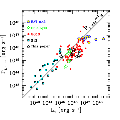
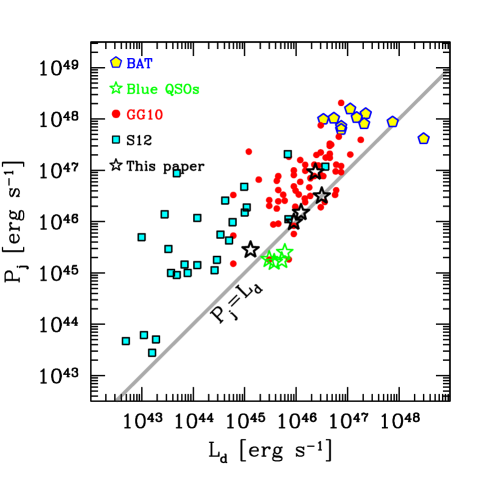
Figure 6: The minimum jet power $P_{\rm j,min}$ (top panel) and the total jet power $P_{\rm j}$ (including one proton per emitting electron), as a function of the accretion luminosity $L_{\rm d}$. Our sources (black stars) are compared with other $\gamma$–ray loud FSRQs studied previously (BAT $z>2$: Ghisellini et al. 2010a; GG10: Ghisellini et al. 2010b; Blue QSOs: Ghisellini et al. 2012; S12: Sbarrato et al. 2012a). The blazars studied in this paper lie on the bulk of the distribution. The minimum jet power is twice the power that the jet spends to produce the radiation we see (i.e. $P_{\rm j,min}=2P_{\rm r}$, see text and Ghisellini & Tavecchio 2010).

5 Discussion and conclusions

With our Swift+GROND observational campaign, we have secured the X–ray coverage for all the blazars at $z>2$ present on the “clean” 2LAC catalog. The use of simultaneous GROND and Swift observations were crucial to find the black hole mass and accretion rate for 3 out of 5 sources (for MG2 J133305+2725 the synchrotron jet component was too strong to see the accretion disc emission, and for PKS 1348+007 our observations cought the source in a very high state, hiding the disc emission that was instead visible by previous SDSS photometric observations). We find that both $M$ and $L_{\rm d}/L_{\rm Edd}$ are not extreme, but rather standard for the powerful FSRQs detected by Fermi/LAT. We have shown that the method of combining broad line luminosities, near IR/optical luminosities (when the disc is visible), and a standard Shakura & Sunyaev (1973) disc emission model is very powerful to find $M$ and $\dot{M}$. With good data, showing the disc emission at its peak, the uncertainty on the black hole mass is less than a factor 2. Since the blazars here studied are $\gamma$–ray emitters, we can also robustly constrain the jet power, since the $\gamma$–ray luminosity, in these blazars, is almost equal to the bolometric one. We can then study in a robust way the link between the accretion and the jet powers.

In §4.2 we discussed the uncertainties related to the jet power, associated to the unknown proton/lepton ratio. One robust lower limit is associated to $P_{\rm r}$, the power that the jet spends to produce the radiation we see. It is simply $P_{\rm r}\sim\Gamma^{2}L_{\rm bol}$ (see Appendix), where $L_{\rm bol}$ is the total jet luminosity. Ghisellini & Tavecchio (2010) have discussed the importance of the Compton rocket effect on the jet when it is crossing the BLR. In the comoving frame of the jet, the seed photons are not isotropically distributed. This implies that also the inverse Compton scattered photons are not isotropic, and more power is emitted in the forward direction (i.e. along the jet velocity direction). The jet then must recoil. If the jet is “heavy” (i.e. one proton per electron) the recoil is negligible, but if the jet is made by pairs the effect is very important. The jet halves its bulk Lorentz factor when there are $\sim$20 pairs per proton. This corresponds to a power that is roughly equal to $P_{\rm r}$. Requiring that the jet does not decelerate significantly, we end up with a minimum jet power (corresponding to a minimum amount of protons) that simply is $P_{\rm j,min}=2P_{\rm r}$. On the other hand, if we assume no pairs and therefore one proton per electron, we have a jet power $P_{\rm j}$.

These two quantities are listed in the two last columns of Tab. 7. Fig. 6 shows $P_{\rm j,min}$ (top panel) and $P_{\rm j}$ (bottom panel) as a function of $L_{\rm d}$ for our blazars, where they are compared to other powerful FSRQs that we have analysed in the past. These are the FSRQs at $z>2$ detected by the 3 years all sky survey of Swift/BAT (Ajello et al. 2009, these blazars are labelled BAT $z>2$ in Fig. 6 and were studied by Ghisellini et al. 2010a); the FSRQs detected by Fermi/LAT in the first 3 months of operations (labelled G10; Ghisellini et al. 2010b); the 4 “blue” quasars (FSRQs with a strong synchrotron component peaking in the optical, labelled “Blue QSOs” in Fig. 6, Ghisellini et al. 2012); and all the FSRQs in the 1LAC sample present also in the SDSS spectroscopic survey (labelled S12, Sbarrato et al. 2012a).

Note that:

• Our blazars lie in the bulk of the distribution, with average values of the jet power and accretion luminosity.

• The correlation between $P_{\rm j,min}$ and $L_{\rm d}$ (top panel of Fig. 6) is significantly less dispersed than the $P_{\rm j}$–$L_{\rm d}$ relation. We re–iterate that $P_{\rm j}$ is found considering one proton per emitting electron, so that a non–constant number of pairs per proton could be responsible for the larger dispersion. However, we think it is premature to draw any strong conclusion, given the related uncertainties.

• $P_{\rm j,min}$ is of the same order as $L_{\rm d}$. Given that this jet power is a lower limit, this suggest that the total jet power can be larger than $L_{\rm d}$. In turn, this suggests that the origin of the jet power cannot be accretion only, and favours the extraction of the black hole spin energy as the prime movers of the jet power.

• We can compare the $z<2$ blazar detected by Swift/BAT with the blazar in our sample. It is evident that the former have both more powerful jets and more luminous accretion discs, lying at the higher end of the distribution of powers.

With our observational campaign all the Fermi $z>2$ blazars in the 2LAC catalog have been observed and detected in the Swift/XRT energy range. This allows us to have a conclusive view of the SED of high redshift $\gamma$–ray blazars.

From our results we conclude that Fermi blazars at high redshifts are indeed powerful, but not extreme. Similarly, also their black hole masses are large, but not extreme. This can be contrasted with high–$z$ blazars detected at hard X–ray energies, that all have extreme values of the jet power, of the disc luminosity and of the black hole mass. Therefore the hard X–ray band ($>$30 keV) is more efficient than the $\gamma$–ray band (given the current sensitivities) in finding the most powerful blazars. This is expected if the so called “blazar sequence” (Fossati et al. 1998; Ghisellini et al. 1998) holds even at the highest power, since it predicts that the peak frequencies of both the synchrotron and the high energy humps shift to lower values when increasing the bolometric observed luminosity. At the highest end of the power distribution, the high energy peak can shift to sub–MeV energies, implying a large hard X–ray flux and a smaller $\gamma$–ray flux (with the K–correction working in the same direction).

References

- [] Abdo A.A., Ackermann M., Ajello M. et al., 2010, ApJ, 715, 429
- [] Ackermann M., Ajello M., Allafort A. et al., 2011, ApJ, 743, 171,
- [] Ajello M., Costamante L., Sambruna R.M. et al., 2009, ApJ, 699, 603
- [] Atwood W.B. Abdo A.A. Ackermann M. et al., 2009, ApJ, 697, 1071
- [] Baumgartner W.H. et al., 2010, ApJS, submitted
- [] Burrows D.N., Hill J.E., Nousek J.A., 2005, Space Sci. Rev., 120, 165
- [] Cardelli J.A., Clayton G.C. & Mathis J.S., 1989, ApJ, 345, 245
- [] Cash W. 1979, ApJ, 228, 939
- [] Cusumano G., La Parola V., Segreto A. et al., 2010, A&A, 524, A64
- [] Fossati G., Maraschi L., Celotti A., Comastri A. & Ghisellini G., 1998, MNRAS, 299, 433
- [] Francis P.J., Hewett P.C., Foltz C.B., Chaffee F.H., Weymann R.J. & Morris S.L., 1991, ApJ, 373, 465
- [] Fuhrmann L., Cucchiara A., Marchili N. et al., 2006, A&A, 445, L1
- [] Gehrels N., 1986, ApJ, 303, 336
- [] Gehrels N., Chincarini G., Giommi P. et al., 2004, ApJ, 611, 1005
- [] Ghisellini G., Celotti A., Fossati G., Maraschi L. & Comastri A., 1998, MNRAS, 301, 451
- [] Ghisellini G. & Tavecchio F., 2009, MNRAS, 397, 985
- [] Ghisellini G., Maraschi L. & Tavecchio F., 2009, MNRAS, 396, L105
- [] Ghisellini G. & Tavecchio F., 2010, MNRAS, 409, L79
- [] Ghisellini G., Della Ceca R., Volonteri M. et al., 2010a, MNRAS, 405, 387
- [] Ghisellini G., Tavecchio F., Foschini L., Ghirlanda G., Maraschi L., Celotti A. 2010b, MNRAS, 402, 497
- [] Ghisellini G. Tagliaferri G., Foschini L. et al., 2011, MNRAS, 411, 901
- [] Ghisellini G., Tavecchio F., Foschini L., Sbarrato T., Ghirlanda G. & Maraschi L., 2012, MNRAS, 425, 1371
- [] Giommi P., Blustin A.J., Capalbi M. et al., 2006, A&A, 456, 911
- [] Giommi P., Polenta G., Lähteenmäki A. et al., 2012, A&A, 541, A160
- [] Greiner J. et al. 2008, PASP, 120, 405
- [] Kalberla P.M.W., Burton W.B., Hartmann D., Arnal E.M., Bajaja E., Morras R. & Pöppel W.G.L., 2005, A&A, 440, 775
- [] Katarzynski K. & Ghisellini G., 2007, A&A, 463, 529
- [] Krühler, T., Küpcü Yoldas, Greiner, J. et al., 2008, ApJ, 685, 376
- [] Krühler T., Schady P., Greiner J. et al., 2011, A&A 526, A153
- [] Pian E., Foschini L., Beckmann V. et al., 2006, A&A, 449, L21
- [] Rau A., Schady P., Greiner J. et al., 2012, A&A, 538, A26
- [] Roming P.W.A., Kennedy T.E., Mason K.O. et al., 2005, Space Sci. Rev., 120, 95
- [] Sbarrato T., Ghisellini G., Maraschi L. & Colpi M., 2012a, MNRAS, 421, 1764
- [] Sbarrato T., Ghisellini G., Nardini M. et al., 2012b, MNRAS, in press (astro–ph/1208.3467)
- [] Schlafly E.F. & Finkbeiner D.P., 2011, ApJ, 737, 103
- [] Shakura N.I. & Sunyaev R.A., 1973, A&A, 24, 337
- [] Shaw M.S., Romani R.W., Cotter G. et al., 2012, ApJ, 748, 49
- [] Sikora M. & Madejski G., 2000, ApJ, 534, 109
- [] Skrutskie, M. F., Cutri, R. M., Stiening, R. et al., 2006, AJ, 131, 1163
- [] Smith J.A., Tucker D.L., Kent S. et al., 2002, AJ, 123, 2121
- [] Tchekhovskoy A., Narayan R. & McKinney J.C., 2011, MNRAS, 418, L79
- [] Tody D., 1993, Astronomical Data Analysis Software and Systems II, 52, 173
- [] Vanden Berk D.E., Richards G.T., Bauer A. et al., 2001, AJ, 122, 549
- [] Villata M., Raiteri C.M., Balonek T.J. et al., 2006, A&A, 453, 817
- [] Volonteri M. et al., Haardt F., Ghisellini G. & Della Ceca R., 2011, MNRAS, 416, 216