Production of a gluon with the exchange of three reggeized gluons in the Lipatov effective action approach.

Abstract

In the Regge kinematics the amplitude for gluon production off three scattering centers is found in the Lipatov effective action technique. The vertex for gluon emission with the reggeon splitting in three reggeons is calculated and its transversality is demonstrated. It is shown that in the sum of all contributions terms containing principal value singularities are cancelled and substituted by the standard Feynman poles. These results may be used for calculation of the inclusive cross-section for gluon production on two nucleons in the nucleus.

1 Introduction

The inclusive gluon production on the nucleus is one of the basic processes in high-energy collisions off nuclear targets. In the QCD it can be studied either in the Feynman diagram approach with interacting reggeized gluons  [1] or in the framework of the dipole picture (or equivalent JIMWLK approach with certain approximations) in which the gluon field is substituted by colour dipoles with their density evolving in rapidity  [2]. It is important to compare these two approaches and see if they are completely equivalent or different in some respects. In particular in  [3] it was advocated that the cross-section for the gluon production on two centers found in the framework of the dipole approach in  [2] is not complete and has to be supplemented by new terms involving states composed of three and four reggeized gluons (the so-called BKP states). On the other hand in  [4] it was shown that, at least in lowest orders, contributions from such states in fact cancel, so that one is left with exactly the cross-section obtained in the dipole approach. It should be stressed however that this conclusion was found in the purely transversal approach with the use of the standard AGK relations  [5] for different cuts of the scattering amplitude off the two centers. To finally prove the complete equivalence of the reggeized gluon and dipole approaches one has to compare contributions from all different cuts and check the validity of the mentioned AGK rules. This cannot be done in the purely transverse approach used in  [1, 4] (nor in the dipole approach) but requires knowledge of the amplitude for the intermediate gluon production as a function of its longitudinal momenta. This information is trivial for production on a single scattering center in the target. But it becomes considerably more complicated when the target involves two or more centers.

A powerful and constructive technique for the calculation of all Feynman diagrams in the Regge kinematics is provided by the Lipatov effective action  [6]. In the inclusive production on two centers, in the lowest order, there appear diagrams with production of the observed gluon (P) from the splitting vertex of a reggeized gluon (R) into two or three reggeized gluons, shown in Fig. 1, $a$ and $b$. The splitting vertex R$\to$RRP entering Fig. 1, $a$ was calculated in  [7] and its contribution together with all accompanying ones to the inclusive cross-section was found in  [8]. To finally find the total inclusive cross-section one has to calculate contributions from diagrams of the type Fig. 1,$b$ which involve a still more complicated vertex R$\to$RRRP. This paper is devoted to the study of this vertex and its contribution together with all accompanying diagrams to the production amplitude on the right-hand side of the cut in Fig. 1,$b$.

Figure 1: Diagrams for the inclusive cross-section on two centers

Our study in  [9] has found that the vertex for the splitting of a reggeized gluon into two with emission of a real gluon has two remarkable properties. The first is that it contains all contributions in the Regge kinematics for the emitted gluon. However, contributions from the region in which one of the lower reggeized gluons has the ”$-$” component of its momentum much smaller than the observed gluon lie outside this kinematics and should be added to the vertex. The second is that with the latter contribution added the resulting expression is similar to what is obtained in the purely transverse picture with addition of standard propagators for the intermediate quarks and gluons. This observation settles the problem of light-cone singularities in the Lipatov effective action formulas and substantially simplifies calculation of the inclusive cross-sections.

Our results in this paper show that these properties remain valid when the number of scattering centers is increased to three. We suspect that this result is quite general and remains valid for any number of centers. As for the cross-section to be calculated from Fig. 1,$b$ we hope that it will cancel a considerable part of the calculated terms for Fig. 1,$a$ and lead to a compact expression for the total inclusive cross-section. However, this derivation is postponed for our future publication.

The paper is organized as follows. To make the presentation self-contained, at least to some extent, in the next section we reproduce the main points of the Lipatov effective action formalism and the known expressions for the R$\to$RP and R$\to$RRP vertices together with the mentioned properties of the latter, which we are going to show to be valid also for the R$\to$RRRP vertex. Section 3 is devoted to the derivation of the R$\to$RRRP vertex. In sections 4 and 5 we calculate diagrams with two and three interactions of the projectile which are to be added to the contribution from the R$\to$RRRP vertex. In section 6 we show that in the sum of all diagrams one obtains the result which naively follows from the purely transverse picture with additional Feynman propagators. Finally in Section 7 we draw some conclusions. Certain cumbersome calculations are transferred to Appendices A and B. In Appendix C we demonstrate that the found R$\to$RRRP vertex is gauge invariant.

In our derivation, as in  [7, 9, 8], for simplicity we take quarks as the projectile and nuclear components, invoking colorless exchanges by adequate projectors.

2 The effective action formalism. R$\to$RP and R$\to$RRP vertices

The effective Lagrangian  [6] describes interaction of the quark $\psi$ and gluon $V_{\mu}=-iT^{a}V^{a}_{\mu}$ fields and their interaction with the independent reggeon field $A_{{\mu}}=-iT^{b}A^{b}_{\mu}$ with $A_{\perp}=0$:

$${\cal L}_{eff}={\cal L}_{YM}(v_{\mu})+\bar{\psi}\Big{(}i\hat{\partial}+ig\hat{v}-M\Big{)}\psi+{\rm Tr}\Big{(}({\cal A}_{+}(v_{+})-A_{+})\partial^{2}_{\perp}A_{-}\Big{)}+{\rm Tr}\Big{(}({\cal A}_{-}(v_{-})-A_{-})\partial^{2}_{\perp}A_{+}\Big{)},$$ (1)

where ${\cal L}_{YM}$ is the standard Yang-Mills Lagrangian,

$${\cal A}_{\pm}(v_{\pm})=-\frac{1}{g}\partial_{\pm}\frac{1}{D_{\pm}}\partial_{\pm}*1=\sum_{n=0}^{\infty}(-g)^{n}v_{\pm}(\partial_{\pm}^{-1}v_{\pm})^{n}$$

$$=v_{\pm}-gv_{\pm}\partial_{\pm}^{-1}v_{\pm}+g^{2}v_{\pm}\partial_{\pm}^{-1}v_{\pm}\partial_{\pm}^{-1}v_{\pm}-g^{3}v_{\pm}\partial_{\pm}^{-1}v_{\pm}\partial_{\pm}^{-1}v_{\pm}\partial_{\pm}^{-1}v_{\pm}+\dots$$ (2)

and the shift of the field variable $v_{\mu}=V_{\mu}+A_{\mu}$ is done to exclude direct gluon-reggeon transitions. The unusual two last terms in (1) and correspondent interaction vertices are called ”induced”.

The Lagrangian is assumed to be local in rapidity, that is, all real and virtual particles in the direct channels split into groups in correspondence with their rapidities $y=\frac{1}{2}\ln|p_{+}/p_{-}|$ and the Lagrangian (1) describes only interactions within one group whereas the interaction between groups with essentially different rapidities is realized by reggeon exchange. The field $A_{-}$ interacts with a group of a higher rapidity and the field $A_{+}$ interacts with a group of a smaller rapidity. The reggeon propagator (in momentum representation)

$$<A_{+}^{a}A_{-}^{b}>=-2i\frac{\delta_{ab}}{q_{\perp}^{2}}$$ (3)

corresponds to the exchange of one reggeon. The following kinematical constraints are implied for the reggeon field

$$\partial_{-}A_{+}=0,\quad\partial_{+}A_{-}=0,$$ (4)

which reflect the smallness of correspondent components of reggeon momenta compared to momenta flowing in the group with the given rapidity.

Note that the normalization $a_{\pm}=a_{0}\pm a_{3}=a_{\mu}n^{\pm}_{\mu}$ for longitudinal components of Lorentz vectors is used in this article, with unit vectors $n^{\pm}_{\mu}=(1,0,0,\mp 1)$, thus $a_{\mu}b_{\mu}=\frac{1}{2}a_{+}b_{-}+\frac{1}{2}a_{-}b_{+}+a_{\perp}b_{\perp}$.

Our aim is to calculate the amplitude for the production of a real gluon with momentum $p$ by the projectile quark of the momentum $k$ with three reggeons of momenta $q_{i}$, $i=1,2,3$ interacting with the target quarks. The multi-Regge kinematical constraints for the case of gluon production with the momentum $p=q-\sum_{i}q_{i}$ in the central region are

$$k_{+}=\sqrt{s}\approx k^{\prime}_{+}>>p_{+}\approx q_{+}>>q_{i+}\approx 0,$$

$$\sqrt{s}>>p_{-}\sim q_{i-}>>q_{-}=-k^{\prime}_{-}\approx 0,\quad k_{-}=0,$$

$$k^{\prime}_{\perp}=-q_{\perp}\sim p_{\perp}\sim q_{i\perp}<<\sqrt{s}\,,\quad k_{\perp}=0,$$ (5)

where $k^{\prime}$ is the momentum of the final quark and $q=k-k^{\prime}$ is the transferred momentum. In this kinematics the transferred momentum and the reggeon momenta are almost transverse $q^{2}\approx q_{\perp}^{2}$, $q_{i}^{2}\approx q_{i\perp}^{2}$. Since the relevant momenta are implied to be very large, we can neglect all the masses, so the quark is considered massless ($M=0$).

To carry out calculations for the R$\to$RRRP vertex one has to preliminary know expressions for the R$\to$RP, and the R$\to$RRP vertices or, in fact, for the convolution of these vertices with the polarization vector $\epsilon^{*}$ of the outgoing gluon. Due to the property of transversality of reggeon-gluon vertices with respect to the gluon momentum [6], the polarization vector obeying the relation $(p\epsilon)=0$ can be chosen independently from the choice of gauge for the gluon field (we will use the Feynman gauge). It is most convenient to take the polarization vector satisfying condition $\epsilon_{+}=0$ and parametrized by its transverse components:

$$\epsilon_{\mu}(p)=\epsilon^{\perp}_{\mu}-\frac{(p\epsilon)_{\perp}}{p_{+}}n_{\mu}^{+},\quad\epsilon_{-}(p)=-\frac{2(p\epsilon)_{\perp}}{p_{+}}\ .$$ (6)

The R$\to$RP (Lipatov) vertex in a covariant form is well-known [6]:

$$\frac{gf^{bb_{1}d}}{2}\left[q_{\mu}+q_{1\mu}+\left(\frac{q_{1}^{2}}{q_{+}}-q_{1-}\right)n^{+}_{\mu}+\left(\frac{q^{2}}{q_{1-}}-q_{+}\right)n^{-}_{\mu}\right],$$ (7)

Its convolution with the polarization vector takes a simple form

$$-gf^{bb_{1}d}q_{\perp}^{2}L(p,q_{1}),$$ (8)

where

$$L(p,q_{1})=\frac{(p\epsilon^{*}_{\perp})}{p_{\perp}^{2}}-\frac{(p+q_{1},\epsilon^{*}_{\perp})}{(p+q_{1})_{\perp}^{2}}\,.$$ (9)

The expression for the R$\to$RRP vertex was derived in [7] and its transversality was checked. Its convolution with the polarization vector can be presented in the form

$$ig^{2}f^{cb_{1}d}f^{db_{2}a}\left[-\frac{q_{+}B(p,q_{2},q_{1})}{(q-q_{1})^{2}+i0}+\frac{L(p,q_{2})}{q_{1-}}\right](p+q_{1}+q_{2})_{\perp}^{2}+\Big{(}\mbox{permutation of }q_{1,2}\mbox{ and }b_{1,2}\Big{)},$$ (10)

where $B$ is the Bartels vertex

$$B(p,q_{2},q_{1})=L(p+q_{2},q_{1})=\frac{(p+q_{2},\epsilon^{*}_{\perp})}{(p+q_{2})_{\perp}^{2}}-\frac{(p+q_{2}+q_{1},\epsilon^{*}_{\perp})}{(p+q_{2}+q_{1})_{\perp}^{2}}\,.$$ (11)

The pole in $q_{1-}$ in the second term in square brackets in (10) is to be understood in the sense of principal value.

Passing to the production amplitude on the right-hand side of the cut in Fig. 1,$a$ one takes into account that the vertex for the interaction of a projectile quark is

$$ig\frac{\gamma_{+}}{2}T^{b}\,.$$ (12)

To this production amplitude also two diagrams with a double interaction of the projectile quark, shown in Fig. 2, give a contribution, from which only terms proportional to $\delta(2k_{+}q_{1,2-})$ in the projectile quark propagator should be taken into account [9].

Figure 2: Diagrams with a double reggeon exchange.

However, remarkably the rest of the terms in these amplitudes give the contribution which identically coincides with the second term in square brackets in (10). So, as stated in the Introduction, one may drop this second term containing the principal value singularity and instead take the diagrams with the double projectile quark interaction with full Feynman propagator for the intermediate projectile quark.

3 Effective R$\to$RRRP vertex

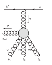
Figure 3: A diagram with a single interaction of the projectile.

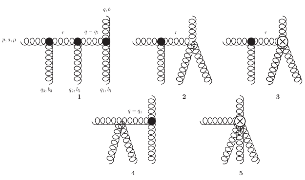
Figure 4: Diagrams of the R$\to$RRRP effective vertex.

The contribution of the full effective R$\to$RRRP vertex to the gluon production amplitude with three reggeons attached to the target is shown in Fig. 3 , where the vertex is marked as a filled blob. In fact the full vertex is a sum of several diagrams of the effective theory which are presented in Fig. 4. In all diagrams horizontal curly lines correspond to real or virtual gluons, vertical curly lines correspond to reggeons and straight lines with arrows correspond to quarks. The effective vertex is implied to be symmetrical with respect to all permutations of the three lower (”induced”) reggeons, so that full symmetrization with respect to reggeon momenta and colour indices has to be carried out for each diagram from Fig. 4.

For brevity in the expressions for all diagrams the common factor corresponding to the three propagators of induced reggeons $8/(q^{2}_{1\perp}q^{2}_{2\perp}q^{2}_{3\perp})$ will be suppressed in this and subsequent sections.

3.1 Diagram 1

Diagram 1 from Fig. 4 has to be obtained by convolution of two ”gluon$\to$reggeon$+$gluon” (P$\to$RP) vertices and two propagators of virtual gluons with the Lipatov vertex (7). For the P$\to$RP vertex we use Eq.(31) from [7] which is in our case:

$$\frac{gf^{b_{3}ad}}{2}\Big{(}-2p_{+}g_{\mu\sigma}+(p+2q_{3})_{\mu}n^{+}_{\sigma}+(p-q_{3})_{\sigma}n^{+}_{\mu}+\frac{q_{3}^{2}}{p_{+}}n^{+}_{\mu}n^{+}_{\sigma}\Big{)},$$ (13)

where the virtual gluon momentum $r=q-q_{1}-q_{2}=p+q_{3}$ has longitudinal components $r_{+}=p_{+}=q_{+}$ and $r_{-}=-q_{1-}-q_{2-}$, and we take gluon propagators in the Feynman gauge. Thus, the expression for the diagram is found to be

$$\epsilon^{*}_{\mu}\cdot\frac{gf^{b_{3}ad}}{2}\Big{(}-2p_{+}g_{\mu\sigma}+(p+2q_{3})_{\mu}n^{+}_{\sigma}+(p-q_{3})_{\sigma}n^{+}_{\mu}+\frac{q_{3}^{2}}{p_{+}}n^{+}_{\mu}n^{+}_{\sigma}\Big{)}$$

$$\times\frac{-i}{(q-q_{1}-q_{2})^{2}+i0}\cdot\frac{gf^{b_{2}dc}}{2}\Big{(}-2r_{+}g_{\sigma\lambda}+(r+2q_{2})_{\sigma}n^{+}_{\lambda}+(r-q_{2})_{\lambda}n^{+}_{\sigma}+\frac{q_{2}^{2}}{r_{+}}n^{+}_{\sigma}n^{+}_{\lambda}\Big{)}$$

$$\times\frac{-i}{(q-q_{1})^{2}+i0}\cdot\frac{gf^{bb_{1}c}}{2}\left[q_{\lambda}+q_{1\lambda}+\left(\frac{q_{1}^{2}}{q_{+}}-q_{1-}\right)n^{+}_{\lambda}+\left(\frac{q^{2}}{q_{1-}}-q_{+}\right)n^{-}_{\lambda}\right]$$

$$=\frac{g^{3}f^{bb_{1}c}f^{cb_{2}d}f^{db_{3}a}}{((q-q_{1})^{2}+i0)((q-q_{1}-q_{2})^{2}+i0)}\left[-q_{+}^{2}(q_{1}\epsilon^{*}+p\epsilon^{*}_{\perp}+q_{2}\epsilon^{*}+q_{3}\epsilon^{*})+\frac{q_{+}q_{\perp}^{2}}{q_{1-}}\cdot(p+q_{2}+q_{3})\epsilon^{*}_{\perp}\right].$$ (14)

Using the identities $(q_{i}\epsilon)=(q_{i}\epsilon)_{\perp}$, $i=1,2,3$ and $(p\epsilon)=0$ we get the final expression for the first diagram from Fig. 4:

$$\frac{g^{3}f^{bb_{1}c}f^{cb_{2}d}f^{db_{3}a}}{((q-q_{1})^{2}+i0)((q-q_{1}-q_{2})^{2}+i0)}\left[-q_{+}^{2}(q\epsilon^{*})_{\perp}+\frac{q_{+}q_{\perp}^{2}}{q_{1-}}\cdot(q-q_{1})\epsilon^{*}_{\perp}\right],$$ (15)

to which analogous terms with all simultaneous permutations of momenta $q_{1,2,3}$ and colour indices $b_{1,2,3}$ of induced reggeons have to be added.

3.2 Diagrams 2 and 3

The diagrams 2 and 3 from Fig. 4 are similar, the only difference between them is that the diagram 2 contains the standard quadruple vertex R$\to$RRP coming from the first term in (1) and diagram 3 contains the induced vertex R$\to$RRP coming from the remaining terms. To calculate the sum of these diagrams we need to know the expression for the sum of the quadruple and the induced vertices, which was already written in [7] (Eq.(26) there):

$$\frac{ig^{2}}{4}\left[f^{bb_{1}c}f^{cb_{2}d}\Big{(}\frac{2q_{\perp}^{2}n_{\sigma}^{-}}{r_{-}q_{1-}}-n_{\sigma}^{+}\Big{)}+f^{bb_{2}c}f^{cb_{1}d}\Big{(}\frac{2q_{\perp}^{2}n_{\sigma}^{-}}{r_{-}q_{2-}}-n_{\sigma}^{+}\Big{)}\right],$$ (16)

where $r_{-}=-q_{1-}-q_{2-}$. This expression is symmetrical with respect to permutation of reggeons 1 and 2, therefore, taking into account the subsequent symmetrization over all permutations of the induced reggeons, it is sufficient to consider only the first term in the square brackets (one half of the vertex).

Convoluting the P$\to$RP vertex (13), the gluon propagator and (16), we get

$$\epsilon^{*}_{\mu}\cdot\frac{gf^{b_{3}ad}}{2}\Big{(}-2p_{+}g_{\mu\sigma}+(p+2q_{3})_{\mu}n^{+}_{\sigma}+(p-q_{3})_{\sigma}n^{+}_{\mu}+\frac{q_{3}^{2}}{p_{+}}n^{+}_{\mu}n^{+}_{\sigma}\Big{)}$$

$$\times\frac{-i}{(q-q_{1}-q_{2})^{2}+i0}\cdot\frac{ig^{2}}{4}f^{bb_{1}c}f^{cb_{2}d}\left[-\frac{2q_{\perp}^{2}n_{\sigma}^{-}}{(q_{1}+q_{2})_{-}q_{1-}}-n_{\sigma}^{+}\right]$$

$$=-\frac{g^{3}f^{bb_{1}c}f^{cb_{2}d}f^{db_{3}a}}{(q-q_{1}-q_{2})^{2}+i0}\cdot\frac{q_{\perp}^{2}((q-q_{1}-q_{2})\epsilon^{*}_{\perp})}{q_{1-}(q_{1-}+q_{2-})}\,.$$ (17)

3.3 Diagram 4

The diagram 4 from Fig. 4 contains a new ”gluon$\to$2 reggeons+gluon” vertex (P$\to$RRP). The relevant term of the Lagrangian arises from the usual Yang-Mills quadruple interaction

$$\frac{g^{2}}{2}tr\left([v_{\mu},v_{\lambda}][v_{\mu},v_{\lambda}]\right)=\frac{g^{2}}{4}tr\left([v_{+},v_{-}][v_{-},v_{+}]\right)+\cdots$$

$$=-\frac{g^{2}}{4}tr\left([V_{+},A_{-}][V_{+},A_{-}]\right)+\cdots=-\frac{g^{2}}{8}f^{cb_{2}d}f^{db_{3}a}V_{+}^{a}V_{+}^{c}A_{-}^{b_{2}}A_{-}^{b_{3}}+\cdots$$ (18)

and gives the vertex

$$-i\frac{g^{2}}{4}\left(f^{cb_{2}d}f^{db_{3}a}+f^{cb_{3}d}f^{db_{2}a}\right)n^{+}_{\mu}n^{+}_{\lambda}$$ (19)

after symmetrization with respect to permutations of gluons and reggeons. This is the full vertex, since the term $<A_{-}A_{-}V_{\mu}V_{\lambda}>$ is absent in the induced part of (1).

It turns out that in our gauge the diagram 4 from Fig. 4 gives zero contribution, because the convolution

$$\epsilon^{*}_{\mu}\cdot\frac{-ig^{2}}{4}\left(f^{cb_{2}d}f^{db_{3}a}+f^{cb_{3}d}f^{db_{2}a}\right)n^{+}_{\mu}n^{+}_{\lambda}$$

$$\times\frac{-i}{(q-q_{1})^{2}+i0}\cdot\frac{gf^{bb_{1}c}}{2}\left[q_{\lambda}+q_{1\lambda}+\left(\frac{q_{1}^{2}}{q_{+}}-q_{1-}\right)n^{+}_{\lambda}+\left(\frac{q^{2}}{q_{1-}}-q_{+}\right)n^{-}_{\lambda}\right]$$ (20)

is proportional to $\epsilon^{*}_{+}=0$.

3.4 Diagram 5

The diagram 5 from Fig. 4 contains the induced vertex $V_{5}^{ind}=<A_{+}^{b}(q)V_{-}^{a}(p)A_{-}^{b_{1}}(q_{1})A_{-}^{b_{2}}(q_{2})A_{-}^{b_{3}}(q_{3})>$ (R$\to$RRRP) arising only from the induced term

$$-g^{3}tr(A_{+}\partial^{2}_{\perp}v_{-}\partial^{-1}_{-}v_{-}\partial^{-1}_{-}v_{-}\partial^{-1}_{-}v_{-})$$ (21)

of the Lagrangian density (1) of the effective theory. Here $v_{-}=V_{-}+A_{-}$ and the linear in $V_{-}$ part has to be extracted:

$$-g^{3}tr(A_{+}\partial^{2}_{\perp}V_{-}\partial^{-1}_{-}A_{-}\partial^{-1}_{-}A_{-}\partial^{-1}_{-}A_{-})-g^{3}tr(A_{+}\partial^{2}_{\perp}A_{-}\partial^{-1}_{-}V_{-}\partial^{-1}_{-}A_{-}\partial^{-1}_{-}A_{-})$$

$$-g^{3}tr(A_{+}\partial^{2}_{\perp}A_{-}\partial^{-1}_{-}A_{-}\partial^{-1}_{-}V_{-}\partial^{-1}_{-}A_{-})-g^{3}tr(A_{+}\partial^{2}_{\perp}A_{-}\partial^{-1}_{-}A_{-}\partial^{-1}_{-}A_{-}\partial^{-1}_{-}V_{-})\,.$$ (22)

It seems to be convenient to denote the momentum $q_{4}=p$ and the colour index $b_{4}=a$, then the relation $q_{1-}+q_{2-}+q_{3-}+q_{4-}=q_{1-}+q_{2-}+q_{3-}+p_{-}=0$ is fulfilled. In this notation the induced vertex is symmetrical with respect to the simultaneous permutation of corresponding momenta $q_{1,2,3,4}$ and indices $b_{1,2,3,4}$. There are 24 terms, the typical one has the form

$$\frac{tr(T^{b}T^{b_{1}}T^{b_{2}}T^{b_{3}}T^{b_{4}})}{(q_{2-}+q_{3-}+q_{4-})(q_{3-}+q_{4-})q_{4-}}=-\frac{tr(T^{b}T^{b_{1}}T^{b_{2}}T^{b_{3}}T^{b_{4}})}{q_{1-}(q_{3-}+q_{4-})q_{4-}}\ .$$ (23)

Their calculation is straightforward but requires cumbersome algebraic transformations of colour factors. So this calculation is transferred to Appendix A. The resulting induced vertex is found to be

$$V_{5}^{ind}=g^{3}\frac{(p\epsilon^{*})_{\perp}}{p^{2}_{\perp}}q^{2}_{\perp}\left(\frac{f^{bb_{1}c}f^{cb_{2}d}f^{db_{3}a}}{q_{1-}(q_{1-}+q_{2-})}+\Big{(}\mbox{permutations of }q_{1,2,3}\mbox{ and }b_{1,2,3}\Big{)}\right)\,.$$ (24)

3.5 Full effective R$\to$RRRP vertex

The sum of all diagrams in Fig. 4 is thus found to be

$$g^{3}f^{bb_{1}c}f^{cb_{2}d}f^{db_{3}a}$$

$$\times\left[-q_{+}^{2}\frac{(q\epsilon^{*}_{\perp})}{((q-q_{1})^{2}+i0)((q-q_{1}-q_{2})^{2}+i0)}+q_{+}\frac{q_{\perp}^{2}\cdot(q-q_{1})\epsilon^{*}_{\perp}}{((q-q_{1})^{2}+i0)((q-q_{1}-q_{2})^{2}+i0)q_{1-}}\right.$$

$$\left.-\frac{q_{\perp}^{2}\cdot(q-q_{1}-q_{2})\epsilon^{*}_{\perp}}{(q-q_{1}-q_{2})^{2}+i0)(q_{1-}+q_{2-})q_{1-}}+\frac{(p\epsilon^{*}_{\perp})}{p_{\perp}^{2}}\cdot\frac{q_{\perp}^{2}}{q_{1-}(q_{1-}+q_{2-})}\right]$$ (25)

plus 5 other terms with simultaneous permutations of momenta $q_{1,2,3}$ and colour indices $b_{1,2,3}$ of induced reggeons.

One can show that the full R$\to$RRRP vertex is transversal. This is proven in Appendix C by direct calculation.

For future use we rewrite this result in the manner similar to the one in [9], separating terms with causal and principal value singularities. Using the identities

$$\frac{1}{((q-q_{1})^{2}+i0)q_{1-}}=\frac{q_{+}}{(q-q_{1})_{\perp}^{2}((q-q_{1})^{2}+i0)}+\frac{1}{(q-q_{1})_{\perp}^{2}q_{1-}}\,,$$

$$\frac{1}{((q-q_{1}-q_{2})^{2}+i0)(q_{1-}+q_{2-})}=\frac{q_{+}}{(q-q_{1}-q_{2})_{\perp}^{2}((q-q_{1}-q_{2})^{2}+i0)}+\frac{1}{(q-q_{1}-q_{2})_{\perp}^{2}(q_{1-}+q_{2-})}\,,$$ (26)

the full contribution from diagrams with the R$\to$RRRP vertex can be rewritten as a sum of three terms:

$$A_{I}=g^{4}\gamma_{+}T^{b}f^{bb_{1}c}f^{cb_{2}d}f^{db_{3}a}\left(W_{I}+Q_{I}+R_{I}\right)+\Big{(}\mbox{permutations of }q_{1,2,3}\mbox{ and }b_{1,2,3}\Big{)}.$$ (27)

Here

$$W_{I}=\frac{q_{+}^{2}B(p,q_{3}+q_{2},q_{1})}{((q-q_{1})^{2}+i0)((q-q_{1}-q_{2})^{2}+i0)}\,,$$ (28)

$$Q_{I}=-\frac{q_{+}B(p,q_{3},q_{2})}{q_{1-}((q-q_{1}-q_{2})^{2}+i0)}\,,$$ (29)

$$R_{I}=\frac{L(p,q_{3})}{q_{1-}(q_{1-}+q_{2-})}\,.$$ (30)

To finally sum all different contributions in Section 6 it will be convenient to present the colour factor in (27) in the form

$$T^{b}f^{bb_{1}c}f^{cb_{2}d}f^{db_{3}a}=\frac{1}{i}[T^{b_{1}},T^{c}]f^{cb_{2}d}f^{db_{3}a}=-[T^{b_{1}},[T^{b_{2}},T^{d}]]f^{db_{3}a}$$

$$=(T^{b_{2}}T^{d}T^{b_{1}}+T^{b_{1}}T^{d}T^{b_{2}}-T^{d}T^{b_{2}}T^{b_{1}}-T^{b_{1}}T^{b_{2}}T^{d})f^{db_{3}a}.$$ (31)

3.6 Special kinematical regions

The vertex R$\to$RRRP calculated in the previous subsection describes production of a gluon on three centers for arbitrary relations between $p_{-}$ and $q_{i-}$, i=1,2,3. In special cases, for particular relations between these components, it may simplify, degenerating into simpler diagrams containing triple and quadruple reggeon vertices, as illustrated in Fig. 5, 6.

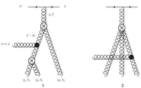
Figure 5: Examples of diagrams with the three-reggeon and with the four-reggeon vertex.

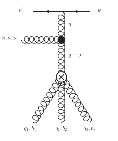
Figure 6: A diagram essential in the kinematics $q_{1-}+q_{2-}+q_{3-}=0$.

For example, under condition

$$|q_{1-}|,|q_{2-}|>>|q_{1-}+q_{2-}|\equiv|q_{3-}+p_{-}|$$ (32)

and as a consequence $q_{1-}+q_{2-}=0$ the general R$\to$RRRP vertex reduces to two diagrams shown in Fig. 5.

Of special interest is the kinematical region in which $p_{-}<<|q_{i-}|$, $i=1,2,3$. As argued in [8], this regime is essential for the calculation of the inclusive gluon production from the heavy nucleus. In this case the momentum $p_{-}$ has to be neglected compared to all other ”$-$” components and can be put to zero. So one needs the production amplitude in the limit

$$q_{1-}+q_{2-}+q_{3-}=0,$$ (33)

where $q_{1,2,3-}\neq 0$.

In this limit $q_{+}\approx p_{+}=-\frac{p_{\perp}^{2}}{p_{-}}$ is very large, so denominators in Eqs.(28)-(30) can be simplified:

$$(q-q_{1})^{2}=-q_{+}q_{1-}+(q-q_{1})_{\perp}^{2}\approx-q_{+}q_{1-}\ ,$$

$$(q-q_{1}-q_{2})^{2}=-q_{+}(q_{1-}+q_{2-})+(q-q_{1}-q_{2})_{\perp}^{2}\approx-q_{+}(q_{1-}+q_{2-}).$$ (34)

Thus we get

$$W_{I}+Q_{I}+R_{I}$$

$$=\frac{q_{+}^{2}B(p,q_{3}+q_{2},q_{1})}{(-q_{+}q_{1-})(-q_{+}(q_{1-}+q_{2-}))}-\frac{q_{+}B(p,q_{3},q_{2})}{q_{1-}(-q_{+}(q_{1-}+q_{2-}))}+\frac{L(p,q_{3})}{q_{1-}(q_{1-}+q_{2-})}$$

$$=\frac{B(p,q_{3}+q_{2},q_{1})+B(p,q_{3},q_{2})+L(p,q_{3})}{q_{1-}(q_{1-}+q_{2-})}\ ,$$ (35)

to which, after multiplying by the colour factor, all permutations of $q_{1,2,3}$ and $b_{1,2,3}$ have to be added. Using the definitions of the Lipatov and Bartels vertices one can write

$$B(p,q_{3}+q_{2},q_{1})+B(p,q_{3},q_{2})+L(p,q_{3})=\frac{(p\epsilon^{*}_{\perp})}{p_{\perp}^{2}}-\frac{(q\epsilon^{*}_{\perp})}{q_{\perp}^{2}}=L(p,q_{1}+q_{2}+q_{3}),$$ (36)

then (35) takes the form

$$\frac{L(p,q_{1}+q_{2}+q_{3})}{q_{1-}(q_{1-}+q_{2-})}\ .$$ (37)

Taking into account colour factors and the symmetrization with respect to induced reggeons (37) gives the following contribution to the production amplitude

$$g^{4}\gamma_{+}L(p,q_{1}+q_{2}+q_{3})T^{b}\left(\frac{f^{bb_{1}c}f^{cb_{2}d}f^{db_{3}a}}{q_{1-}(q_{1-}+q_{2-})}+\frac{f^{bb_{2}c}f^{cb_{3}d}f^{db_{1}a}}{q_{2-}(q_{2-}+q_{3-})}\right.$$

$$\left.+\frac{f^{bb_{3}c}f^{cb_{1}d}f^{db_{2}a}}{q_{3-}(q_{1-}+q_{3-})}+\frac{f^{bb_{2}c}f^{cb_{1}d}f^{db_{3}a}}{q_{2-}(q_{1-}+q_{2-})}+\frac{f^{bb_{1}c}f^{cb_{3}d}f^{db_{2}a}}{q_{1-}(q_{1-}+q_{3-})}+\frac{f^{bb_{3}c}f^{cb_{2}d}f^{db_{1}a}}{q_{3-}(q_{2-}+q_{3-})}\right)\ .$$ (38)

If the condition $q_{1-}+q_{2-}+q_{3-}=0$ is fulfilled, with the use of relations $q_{1-}+q_{3-}=-q_{2-}$, $q_{2-}+q_{3-}=-q_{1-}$ and

$$\frac{1}{q_{1-}(q_{1-}+q_{3-})}=\frac{1}{q_{2-}(q_{2-}+q_{3-})}=-\frac{1}{q_{1-}(q_{1-}+q_{2-})}-\frac{1}{q_{2-}(q_{1-}+q_{2-})}$$

one can rewrite (38) as the sum of two longitudinal momentum structures:

$$g^{4}\gamma_{+}L(p,q_{1}+q_{2}+q_{3})T^{b}\cdot\frac{f^{bb_{1}c}f^{cb_{2}d}f^{db_{3}a}+f^{bb_{3}c}f^{cb_{2}d}f^{db_{1}a}-f^{bb_{2}c}f^{cb_{3}d}f^{db_{1}a}-f^{bb_{1}c}f^{cb_{3}d}f^{db_{2}a}}{q_{1-}(q_{1-}+q_{2-})}$$

$$+\Big{(}\mbox{permutation of }q_{1,2}\mbox{ and }b_{1,2}\Big{)}.$$ (39)

The Jacobi identities $f^{cb_{2}d}f^{db_{3}a}=f^{cb_{3}d}f^{db_{2}a}+f^{cad}f^{db_{3}b_{2}}$ and $f^{bb_{3}c}f^{cb_{2}d}=f^{bb_{2}c}f^{cb_{3}d}-f^{bdc}f^{cb_{3}b_{2}}$ allow us to simplify (39):

$$g^{4}\gamma_{+}L(p,q_{1}+q_{2}+q_{3})T^{b}\cdot\frac{f^{bb_{1}c}f^{cad}f^{db_{3}b_{2}}-f^{bdc}f^{cb_{3}b_{2}}f^{db_{1}a}}{q_{1-}(q_{1-}+q_{2-})}$$

$$+\Big{(}\mbox{permutation of }q_{1,2}\mbox{ and }b_{1,2}\Big{)}.$$ (40)

If we interchange indices of summation $c$ and $d$ in the second term of the numerator, we get the expression proportional to another Jacobi identity $f^{bb_{1}c}f^{cad}-f^{bcd}f^{cb_{1}a}=f^{bac}f^{cb_{1}d}$, and then the full contribution to the amplitude from diagrams with the R$\to$RRRP vertex in the kinematics $q_{1-}+q_{2-}+q_{3-}=0$ takes the form

$$g^{4}\gamma_{+}L(p,q_{1}+q_{2}+q_{3})T^{b}\frac{f^{bac}f^{cb_{1}d}f^{db_{3}b_{2}}}{q_{1-}(q_{1-}+q_{2-})}+\Big{(}\mbox{permutation of }q_{1,2}\mbox{ and }b_{1,2}\Big{)}.$$ (41)

This expression exactly coincides with the contribution of the diagram from Fig. 6 calculated in Appendix B.

In general, diagrams with multi-reggeon effective vertices give a contribution only when the reggeon momenta are restricted by specific kinematical conditions (see [9]). To find these conditions, the equations $\partial_{-}A_{+}=0$ and $\partial_{+}A_{-}=0$ have to be applied to reggeon fields interacting by means of the multi-reggeon vertex. For example, for the first diagram from Fig. 5 with the use of the equation $\partial_{-}A_{+}=0$ for the three-reggeon vertex we get the momentum condition

$$q_{1-}+q_{2-}=0,$$ (42)

which should be understood not as strict equation but as the restriction (32). From the equation $\partial_{+}A_{-}=0$ the conditions $q_{1+}=0$ and $q_{2+}=0$ follow which are always assumed in the Regge kinematics. The relevant momentum condition for the diagram from Fig. 6 with the vertex R$\to$RRR is (33) and it is the only diagram for this kinematics.

4 Double interaction of the projectile

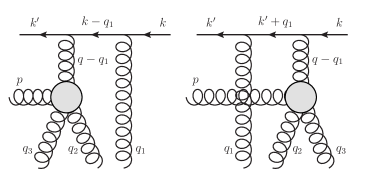
Figure 7: Diagrams with a double interaction of the projectile and the gluon emitted from the R$\to$RRP vertex.

Diagrams with two interactions of the projectile separate into two groups with emission of the gluon from the R$\to$RRP vertex shown in Fig. 7 and from a reggeon shown in Fig. 8.

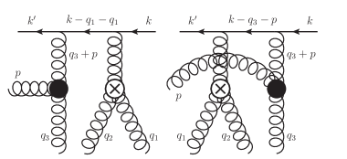
Figure 8: Diagrams with a double interactions of the projectile and the gluon emitted from the R$\to$RP vertex.

4.1 Diagrams in Fig. 7

We start with diagrams in Fig. 7. In both diagrams the filled blob corresponds to the R$\to$RRP vertex. Since the gluon is produced by this vertex we need to know only the convolution of the vertex with the polarization vector. It is given by (10), for diagrams from Fig. 7 the vertex is

$$ig^{2}f^{cb_{2}d}f^{db_{3}a}\left[-\frac{q_{+}B(p,q_{3},q_{2})}{(q-q_{1}-q_{2})^{2}+i0}+\frac{L(p,q_{3})}{q_{2-}}\right](q-q_{1})_{\perp}^{2}+\Big{(}\mbox{permutation of }q_{2,3}\mbox{ and }b_{2,3}\Big{)}\,.$$ (43)

Since the R$\to$RRP vertex is already symmetrical with respect to permutation of the two induced reggeons, the symmetrization for diagrams in Fig. 7 have to be carried out only for cyclic permutations of momenta $q_{1,2,3}$ and colour indices $b_{1,2,3}$.

Note an important point. As argued in [9], from the property of locality in rapidity, it follows that propagators of the virtual quark in diagrams such as in Fig. 7 are to be substituted by their parts proportional to the $\delta$-function. Thus, we have to write for the quark propagators

$$\frac{k_{+}}{(k-q_{1})^{2}+i0}\approx\frac{k_{+}}{-k_{+}q_{1-}+(k-q_{1})_{\perp}^{2}+i0}$$

$$\approx\frac{k_{+}}{-k_{+}q_{1-}+i0}=-P\frac{1}{q_{1-}}-i\pi\delta(q_{1-})\to-i\pi\delta(q_{1-})$$ (44)

and

$$\frac{k^{\prime}_{+}}{(k^{\prime}+q_{1})^{2}+i0}\approx\frac{k_{+}}{k_{+}q_{1-}+(k^{\prime}+q_{1})_{\perp}^{2}+i0}$$

$$\approx\frac{k_{+}}{k_{+}q_{1-}+i0}=P\frac{1}{q_{1-}}-i\pi\delta(q_{1-})\to-i\pi\delta(q_{1-}).$$ (45)

The reason is that the application of the condition of the similarity of rapidities of the scattered quarks and the virtual quark is equivalent to the momentum cut-off which makes the pole term of the propagator tend to zero in the sense of generalized function. The remaining term with the delta-function $-i\pi\delta(q_{1-})$ can be treated as the effective propagator of a quark moving with a high rapidity.

The fermionic part of the first diagram from Fig. 7 including the numerator of quark propagators and quark-reggeon vertices is

$$(ig)^{2}\frac{\gamma_{+}}{2}i(\hat{k}-\hat{q_{1}})\frac{\gamma_{+}}{2}=-ig^{2}\frac{\gamma_{+}}{2}(k_{+}-q_{1+})\approx\frac{-i}{2}g^{2}k_{+}\gamma_{+}\,,$$ (46)

where the identities $\gamma_{+}\gamma_{+}=0$, $\gamma_{+}\gamma_{-}\gamma_{+}=4\gamma_{+}$ are used. The fermionic part of the second diagram from Fig. 7 is identical to (46). Multiplying this expression by the propagator of virtual reggeon $-2i/(q-q_{1})_{\perp}^{2}$ and by the common factor $(q-q_{1})_{\perp}^{2}$ from (43) we get $-g^{2}k_{+}\gamma_{+}$.

Since the effective quark propagators are the same for both diagrams in Fig. 7, their momentum factors are identical and these diagrams differ only by colour factors, which are

$$T^{c}T^{b_{1}}f^{cb_{2}d}f^{db_{3}a}=-i[T^{b_{2}},T^{d}]T^{b_{1}}f^{db_{3}a}=-if^{db_{3}a}(T^{b_{2}}T^{d}T^{b_{1}}-T^{d}T^{b_{2}}T^{b_{1}}).$$ (47)

for the first diagram and

$$T^{b_{1}}T^{c}f^{cb_{2}d}f^{db_{3}a}=-iT^{b_{1}}[T^{b_{2}},T^{d}]f^{db_{3}a}=-if^{db_{3}a}(T^{b_{1}}T^{b_{2}}T^{d}-T^{b_{1}}T^{d}T^{b_{2}})$$ (48)

for the second one.

Collecting all factors and taking into account the symmetrization with respect to induced reggeons, we get the full result for the contribution from diagrams with a double interaction of the projectile and the gluon emitted from the R$\to$RRP vertex:

$$g^{4}\gamma_{+}f^{db_{3}a}(T^{b_{2}}T^{d}T^{b_{1}}-T^{d}T^{b_{2}}T^{b_{1}}+T^{b_{1}}T^{b_{2}}T^{d}-T^{b_{1}}T^{d}T^{b_{2}})$$

$$\times\left[\frac{q_{+}B(p,q_{3},q_{2})}{(q-q_{1}-q_{2})^{2}+i0}-\frac{L(p,q_{3})}{q_{2-}}\right](-i\pi\delta(q_{1-}))$$

$$+\Big{(}\mbox{permutations of }q_{1,2,3}\mbox{ and }b_{1,2,3}\Big{)}.$$ (49)

In the following the first term in square brackets in (49) is referred to as $W_{II}$ and the second one as $R_{II}$.

4.2 Diagrams in Fig. 8

Passing to the diagrams in Fig. 8 (with all permutations of the induced reggeons) we note that the three-reggeon vertex R$\to$RR was calculated in [9], but the other normalization of the ”$\pm$” components was chosen there, so we re-derive the expression. The relevant term of the effective Lagrangian which arises only from the induced term is

$$(-g)tr(A_{+}\partial_{\perp}^{2}A_{-}\partial_{-}^{-1}A_{-})=-\frac{g}{2}tr(A_{+}\partial_{\perp}^{2}[A_{-},(\partial_{-}^{-1}A_{-})])$$

$$=\frac{g}{4}f^{cb_{1}b_{2}}A_{+}^{c}\partial_{\perp}^{2}A_{-}^{b_{1}}(\partial_{-}^{-1}A_{-}^{b_{2}})\,.$$ (50)

The vertex in momentum representation

$$\frac{gf^{cb_{1}b_{2}}}{4}\,(q_{1}+q_{2})_{\perp}^{2}\left(\frac{1}{q_{1-}}-\frac{1}{q_{2-}}\right)$$ (51)

is symmetrical with respect to the permutation of the reggeons 1 and 2. Using the condition (42), we can rewrite the vertex (51) in the form

$$\frac{gf^{cb_{1}b_{2}}}{2q_{1-}}(q_{1}+q_{2})_{\perp}^{2}=-\frac{gf^{cb_{1}b_{2}}}{2q_{2-}}(q_{1}+q_{2})_{\perp}^{2}\,.$$ (52)

As stated in [9], the poles in $q_{1-}$ and $q_{2-}$ should be understood in the sense of principal value. Although the three-reggeon vertex gives a non-zero contribution only under condition $q_{1-}+q_{2-}=0$, in the presence of the factor $-i\pi\delta(q_{1-}+q_{2-})$ remaining from the propagator of the virtual quark this condition is always fulfilled. Therefore one have to include the contribution of diagrams from Fig. 8 in a general Regge kinematics.

The fermionic part of both diagrams from Fig. 8 is the same as for diagrams of Section 4.1:

$$\frac{-i}{2}g^{2}k_{+}\gamma_{+}$$ (53)

and the quark propagators are substituted by their delta-functional parts:

$$\frac{k_{+}}{(k-q_{1}-q_{2})^{2}+i0}\approx\frac{1}{-(q_{1-}+q_{2-})+i0}\to-i\pi\delta(q_{1-}+q_{2-})\mbox{ and}$$

$$\frac{k^{\prime}_{+}}{(k-q_{3}-p)^{2}+i0}=\frac{k^{\prime}_{+}}{(k^{\prime}+q_{1}+q_{2})^{2}+i0}\approx\frac{1}{(q_{1-}+q_{2-})+i0}\to-i\pi\delta(q_{1}+q_{2})$$ (54)

for the first and the second diagram respectively. Multiplying this by two propagators of virtual reggeons, the Lipatov vertex

$$-gf^{db_{3}a}(p+q_{3})^{2}_{\perp}L(p,q_{3})$$ (55)

and by the three-reggeon vertex (52) we get the answer

$$-ig^{4}\gamma_{+}f^{db_{3}a}f^{cb_{1}b_{2}}\left(T^{d}T^{c}+T^{c}T^{d}\right)\frac{L(p,q_{3})}{q_{1-}}(-i\pi\delta(q_{1-}+q_{2-}))$$

$$=g^{4}\gamma_{+}f^{db_{3}a}\left(T^{d}T^{b_{2}}T^{b_{1}}-T^{d}T^{b_{1}}T^{b_{2}}+T^{b_{2}}T^{b_{1}}T^{d}-T^{b_{1}}T^{b_{2}}T^{d}\right)\frac{L(p,q_{3})}{q_{1-}}(-i\pi\delta(q_{1-}+q_{2-})),$$ (56)

which is symmetrical with respect to permutation of the reggeons 1 and 2. Under the symmetrization over all permutations of the induced reggeons the full contribution from diagrams with the three-reggeon vertex can be written in the form

$$A_{IV}=g^{4}\gamma_{+}f^{db_{3}a}\left(\frac{T^{d}T^{b_{2}}T^{b_{1}}}{q_{1-}}-\frac{T^{b_{2}}T^{b_{1}}T^{d}}{q_{2-}}\right)L(p,q_{3})(-i\pi\delta(q_{1-}+q_{2-}))$$

$$+\Big{(}\mbox{permutations of }1,2,3\Big{)}.$$ (57)

5 Triple interaction of the projectile

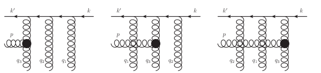
Figure 9: Diagrams with a triple interaction of the projectile.

There are 18 diagrams with three reggeons interacting with the projectile quark. Three of them are shown in Fig. 9, the others can be obtained by means of all permutations of reggeons 1,2,3. The fermionic part of the first diagram from Fig. 9 including the numerators of quark propagators and quark-reggeon vertices is

$$(ig)^{3}\frac{\gamma_{+}}{2}i(\hat{k}-\hat{q_{1}}-\hat{q_{2}})\frac{\gamma_{+}}{2}i(\hat{k}-\hat{q_{1}})\frac{\gamma_{+}}{2}$$

$$=ig^{3}\frac{\gamma_{+}}{2}\left(\frac{1}{2}(k_{+}-q_{1+}-q_{2+})\gamma_{-}\right)\frac{\gamma_{+}}{2}\left(\frac{1}{2}(k_{+}-q_{1+})\gamma_{-}\right)\frac{\gamma_{+}}{2}=\frac{i}{2}g^{3}k_{+}^{2}\gamma_{+}\,.$$ (58)

The other diagrams in Fig. 9 give the same result in the approximation of the Regge kinematics. It has to be multiplied by the propagator of virtual reggeon ${-2i}/{(p+q_{3})^{2}_{\perp}}$ and by the Lipatov vertex (55).

The condition of locality in rapidity has to be applied to the two virtual quarks independently. In correspondence with our notation in the previous section, the full propagator of each quark has to be substituted by its delta-functional part:

$$\frac{k_{+}^{2}}{((k-q_{1}-q_{2})^{2}+i0)((k-q_{1})^{2}+i0)}\approx\frac{1}{(-(q_{1-}+q_{2-})+i0)(-q_{1-}+i0)}\to(-i\pi)^{2}\delta(q_{1-}+q_{2-})\delta(q_{1-}),$$

$$\frac{k^{2}_{+}}{((k^{\prime}+q_{1})^{2}+i0)((k-q_{2})^{2}+i0)}\approx\frac{1}{(q_{1-}+i0)(-q_{2-}+i0)}\to(-i\pi)^{2}\delta(q_{1-})\delta(q_{2-}),$$

$$\frac{k^{2}_{+}}{((k^{\prime}+q_{2})^{2}+i0)((k^{\prime}+q_{1}+q_{2})^{2}+i0)}\approx\frac{1}{(q_{2-}+i0)((q_{1-}+q_{2-})+i0)}\to(-i\pi)^{2}\delta(q_{2-})\delta(q_{1-}+q_{2-})$$ (59)

for the first, second and third diagram from Fig. 9 respectively. Since

$$\delta(q_{1-})\delta(q_{1-}+q_{2-})=\delta(q_{2-})\delta(q_{1-}+q_{2-})=\delta(q_{1-})\delta(q_{2-})\,,$$ (60)

one can see that the momentum factors are identical for the three diagrams in Fig. 9.

Taking into account the colour factors of diagrams in Fig. 9 and the symmetry with respect to all permutations of induced reggeons, we get the full contribution from diagrams with the three reggeon exchange:

$$A_{III}=-g^{4}\gamma_{+}f^{db_{3}a}(T^{d}T^{b_{2}}T^{b_{1}}+T^{b_{1}}T^{d}T^{b_{2}}+T^{b_{2}}T^{b_{1}}T^{d})L(p,q_{3})(-i\pi)^{2}\delta(q_{1-})\delta(q_{2-})$$

$$+\Big{(}\mbox{permutations of }1,2,3\Big{)}.$$ (61)

6 Restoration of causal propagators

Separate parts of the calculated production amplitude contain poles in the ”$-$” longitudinal momenta or their sums, coming from the similar singularity of the induced part of the effective action, whose exact meaning is not fixed apriori. There was a special discussion on this point in  [10, 11], which however was restricted to the simplest case with only one center in the target. In  [9] for the case of two centers in the target, it was established that the correct reproduction of the relevant Feynman diagrams requires these singularities to be interpreted in the principal value sense. Moreover, it was shown that these singularities combined with the $\delta$-functional contributions from double interactions of the projectile turn into the latter with normal causal propagators. In this section, assuming that singularities in ”$-$” components of the momenta are to be interpreted in the principal value sense, we demonstrate that with three centers in the target they also combine into the final expression containing only usual singularities of Feynman diagrams, changing the $\delta$-functions in the propagators of the projectile quark into normal causal propagators.

From diagrams with the single interaction of the projectile we get contribution $W_{I}$ (28)

$$g^{4}\gamma_{+}T^{b}f^{bb_{1}c}f^{cb_{2}d}f^{db_{3}a}\frac{q_{+}^{2}\,B(p,q_{3}+q_{2},q_{1})}{((q-q_{1})^{2}+i0)((q-q_{1}-q_{2})^{2}+i0)}+\Big{(}\mbox{permutations of }1,2,3\Big{)},$$ (62)

which contains only usual Feynman poles.

Next, the principal value pole from the part $Q_{I}$ (29) and the delta-function contribution $W_{II}$ (the first term in square brackets in (49)) from diagrams with a double interaction of the projectile combine into the Feynman pole of the causal propagator:

$$g^{4}\gamma_{+}f^{db_{3}a}\frac{q_{+}B(p,q_{3},q_{2})}{(q-q_{1}-q_{2})^{2}+i0}\,\left[\left(T^{b_{2}}T^{d}T^{b_{1}}-T^{d}T^{b_{2}}T^{b_{1}}\right)\left(-P\frac{1}{q_{1-}}-i\pi\delta(q_{1-})\right)\right.$$

$$+\left.\left(T^{b_{1}}T^{b_{2}}T^{d}-T^{b_{1}}T^{d}T^{b_{2}}\right)\left(P\frac{1}{q_{1-}}-i\pi\delta(q_{1-})\right)\right]+\Big{(}\mbox{permutations of }1,2,3\Big{)}$$

$$\approx g^{4}\gamma_{+}f^{db_{3}a}\frac{q_{+}B(p,q_{3},q_{2})}{(q-q_{1}-q_{2-})^{2}+i0}\!\left[\frac{k_{+}\cdot if^{cb_{2}d}T^{c}T^{b_{1}}}{(k-q_{1})^{2}+i0}+\frac{k_{+}\cdot if^{cb_{2}d}T^{b_{1}}T^{c}}{(k^{\prime}+q_{1})^{2}+i0}\right]\!+\!\Big{(}\mbox{permutations of }1,2,3\Big{)}.$$ (63)

This expression corresponds to the sum of diagrams in Fig. 7 with only the part $W$ of the effective vertex R$\to$RRP taken into account and with the quark propagators taken as a whole.

Finally, we check that the remaining terms, that is the contribution from $R_{I}+R_{II}+A_{III}+A_{IV}$, combine into the expression containing only causal propagators. Note that each of these terms is proportional to the Lipatov vertex. Because of the symmetry with respect to permutation of the induced reggeons, it is sufficient to consider only terms proportional to $L(p,q_{3})$. In subsequent equations all poles in $q_{1,2-}$ and $q_{1-}+q_{2-}$ are understood in the sense of principal value. Then, suppressing the common factor $g^{4}\gamma_{+}f^{db_{3}a}L(p,q_{3})$ we have:

$$R_{I}=\frac{T^{b_{2}}T^{d}T^{b_{1}}+T^{b_{1}}T^{d}T^{b_{2}}-T^{d}T^{b_{2}}T^{b_{1}}-T^{b_{1}}T^{b_{2}}T^{d}}{q_{1-}(q_{1-}+q_{2-})}+\Big{(}\mbox{permutation of }1,2\Big{)},$$

$$R_{II}=-\frac{T^{b_{2}}T^{d}T^{b_{1}}-T^{d}T^{b_{2}}T^{b_{1}}+T^{b_{1}}T^{b_{2}}T^{d}-T^{b_{1}}T^{d}T^{b_{2}}}{q_{2-}}(-i\pi)\delta(q_{1-})+\Big{(}\mbox{permutation of }1,2\Big{)},$$

$$A_{III}=-(T^{d}T^{b_{2}}T^{b_{1}}+T^{b_{1}}T^{d}T^{b_{2}}+T^{b_{2}}T^{b_{1}}T^{d})(-i\pi)^{2}\delta(q_{1-})\delta(q_{2-})+\Big{(}\mbox{permutation of }1,2\Big{)},$$

$$A_{IV}=\left(\frac{T^{d}T^{b_{2}}T^{b_{1}}}{q_{1-}}-\frac{T^{b_{2}}T^{b_{1}}T^{d}}{q_{2-}}\right)(-i\pi)\delta(q_{1-}+q_{2-})+\Big{(}\mbox{permutation of }1,2\Big{)}.$$ (64)

The sum is

$$\frac{T^{b_{2}}T^{d}T^{b_{1}}+T^{b_{1}}T^{d}T^{b_{2}}-T^{d}T^{b_{2}}T^{b_{1}}-T^{b_{1}}T^{b_{2}}T^{d}}{q_{1-}(q_{1-}+q_{2-})}+\frac{T^{b_{1}}T^{d}T^{b_{2}}+T^{b_{2}}T^{d}T^{b_{1}}-T^{d}T^{b_{1}}T^{b_{2}}-T^{b_{2}}T^{b_{1}}T^{d}}{q_{2-}(q_{1-}+q_{2-})}$$

$$+\frac{-T^{b_{2}}T^{d}T^{b_{1}}+T^{d}T^{b_{2}}T^{b_{1}}-T^{b_{1}}T^{b_{2}}T^{d}+T^{b_{1}}T^{d}T^{b_{2}}}{q_{2-}}(-i\pi)\delta(q_{1-})$$

$$+\frac{-T^{b_{1}}T^{d}T^{b_{2}}+T^{d}T^{b_{1}}T^{b_{2}}-T^{b_{2}}T^{b_{1}}T^{d}+T^{b_{2}}T^{d}T^{b_{1}}}{q_{1-}}(-i\pi)\delta(q_{2-})$$

$$+\frac{T^{d}T^{b_{2}}T^{b_{1}}-T^{b_{1}}T^{b_{2}}T^{d}}{q_{1-}}(-i\pi)\delta(q_{1-}+q_{2-})+\frac{T^{d}T^{b_{1}}T^{b_{2}}-T^{b_{2}}T^{b_{1}}T^{d}}{q_{2-}}(-i\pi)\delta(q_{1-}+q_{2-})$$

$$-(T^{d}T^{b_{2}}T^{b_{1}}+T^{b_{1}}T^{d}T^{b_{2}}+T^{b_{2}}T^{b_{1}}T^{d}+T^{d}T^{b_{1}}T^{b_{2}}+T^{b_{2}}T^{d}T^{b_{1}}+T^{b_{1}}T^{b_{2}}T^{d})(-i\pi)^{2}\delta(q_{1-})\delta(q_{2-}).$$ (65)

With the use of the following identities in the sense of the generalized functions

$$\delta(q_{1-})P\frac{1}{q_{2-}}=\delta(q_{1-})P\frac{1}{q_{1-}+q_{2-}}\,,\quad\delta(q_{2-})P\frac{1}{q_{1-}}=\delta(q_{2-})P\frac{1}{q_{1-}+q_{2-}}\,,$$

$$\delta(q_{1-}+q_{2-})P\frac{1}{q_{2-}}=-\delta(q_{1-}+q_{2-})P\frac{1}{q_{1-}}\,,$$

$$\delta(q_{1-})\delta(q_{2-})=\delta(q_{1-})\delta(q_{2-}+q_{1-})=\delta(q_{1-}+q_{2-})\delta(q_{2-}),$$

$$P\frac{1}{q_{1-}}\cdot P\frac{1}{q_{1-}+q_{2-}}+P\frac{1}{q_{2-}}\cdot P\frac{1}{q_{1-}+q_{2-}}=P\frac{1}{q_{1-}}\cdot P\frac{1}{q_{2-}}$$

one can write (65), separating different colour structures, as

$$T^{d}T^{b_{2}}T^{b_{1}}\left(-P\frac{1}{q_{1-}}\cdot P\frac{1}{q_{1-}+q_{2-}}+(-i\pi)\delta(q_{1-})P\frac{1}{q_{1-}+q_{2-}}\right.$$

$$\quad\quad\quad\quad\left.+(-i\pi)\delta(q_{1-}+q_{2-})P\frac{1}{q_{1-}}-(-i\pi)^{2}\delta(q_{1-}+q_{2-})\delta(q_{1-})\right)$$

$$+T^{b_{1}}T^{d}T^{b_{2}}\left(P\frac{1}{q_{1-}}\cdot P\frac{1}{q_{2-}}+(-i\pi)\delta(q_{1-})P\frac{1}{q_{2-}}-(-i\pi)\delta(q_{2-})P\frac{1}{q_{1-}}-(-i\pi)^{2}\delta(q_{1-})\delta(q_{2-})\right)$$

$$+T^{b_{2}}T^{b_{1}}T^{d}\left(-P\frac{1}{q_{2-}}\cdot P\frac{1}{q_{1-}+q_{2-}}-(-i\pi)\delta(q_{2-})P\frac{1}{q_{1-}+q_{2-}}\right.$$

$$\quad\quad\quad\quad\left.-(-i\pi)\delta(q_{1-}+q_{2-})P\frac{1}{q_{2-}}-(-i\pi)^{2}\delta(q_{1-}+q_{2-})\delta(q_{2-})\right)+\Big{(}\mbox{permutation of }1,2\Big{)}$$ (66)

$$=-\frac{T^{d}T^{b_{2}}T^{b_{1}}}{(-(q_{1-}+q_{2-})+i0)(-q_{1-}+i0)}-\frac{T^{b_{1}}T^{d}T^{b_{2}}}{(q_{1-}+i0)(-q_{2-}+i0)}$$

$$-\frac{T^{b_{2}}T^{b_{1}}T^{d}}{(q_{2-}+i0)((q_{1-}+q_{2-})+i0)}+\Big{(}\mbox{permutation of }1,2\Big{)}.$$ (67)

In the approximation of the Regge kinematics the full contribution from $R_{I}+R_{II}+A_{III}+A_{IV}$ is

$$-g^{4}\gamma_{+}f^{db_{3}a}\left[\frac{k_{+}^{2}\cdot T^{d}T^{b_{2}}T^{b_{1}}}{((k-q_{1}-q_{2})^{2}+i0)((k-q_{1})^{2}+i0)}+\frac{k_{+}^{2}\cdot T^{b_{1}}T^{d}T^{b_{2}}}{((k^{\prime}+q_{1})^{2}+i0)((k-q_{2})^{2}+i0)}\right.$$

$$+\left.\frac{k_{+}^{2}\cdot T^{b_{2}}T^{b_{1}}T^{d}}{((k^{\prime}+q_{2})^{2}+i0)((k^{\prime}+q_{1}+q_{2})^{2}+i0)}\right]L(p,q_{3})+\Big{(}\mbox{permutations of }1,2,3\Big{)}.$$ (68)

This corresponds to the sum of diagrams in Fig. 9 with the quark propagators taken as normal Feynman ones.

7 Conclusions

The main result of this paper is the explicit form of the amplitude for the production of a real gluon off three scattering centers, which is given by Eqs. (62), (63) and (68). An essential part of this amplitude is the vertex R$\to$RRRP for the emission of a gluon with the reggeon splitting into three calculated in Section 3. The found amplitude can be used for the calculation of such observables as the inclusive cross-section for gluon jet production on two nucleons in the nucleus and the diffractive gluon production on three nucleons in the nucleus.

Two important properties have been established. First, we have shown that in the sum of all terms principal value singularities in the longitudinal momenta coming from the induced contributions combine with the $\delta$-like singularities in the remaining contributions with multiple interactions of the projectile to restore normal propagators for the latter. So in the end no trace of the principal value prescription remains. Second, we have found that in the kinematics appropriate for the calculation of the inclusive cross-section when the ”$-$” component of the observed gluon momentum is much smaller than the ”$-$” components of the momenta transferred to the target, the vertex R$\to$RRRP is radically simplified and reduced to the contribution of the diagram from Fig. 6. Both results may be useful in the calculation of the inclusive cross-sections.

Note that these properties are quite similar to the ones established earlier for the production on two centers in [9]. This makes us believe that they have a general validity and are fulfilled for any number of scattering centers.

8 Acknowledgments

This work has been partially supported by the RFFI grant 12-02-00356-a .

9 Appendix A. Calculation of the induced vertex

We denote the term

$$\frac{tr(T^{b}T^{b_{1}}T^{b_{2}}T^{b_{3}}T^{b_{4}})}{(q_{2-}+q_{3-}+q_{4-})(q_{3-}+q_{4-})q_{4-}}=-\frac{tr(T^{b}T^{b_{1}}T^{b_{2}}T^{b_{3}}T^{b_{4}})}{q_{1-}(q_{3-}+q_{4-})q_{4-}}$$ (A.1)

as

$$-\frac{[b1234]}{1(3+4)4}$$

for brevity.

We have to calculate the convolution of the induced vertex with the polarization vector of the gluon. Then the common factor

$$-ig^{3}(q^{2}_{\perp})\epsilon^{*}_{-}=ig^{3}\frac{2(p\epsilon^{*})_{\perp}}{p_{+}}q^{2}_{\perp}$$ (A.2)

includes $(-1)$ from (A.1), $i$ for the vertex, $-g^{3}$ from (22), $(-i)^{5}$ from fields, $-q^{2}_{\perp}$ from $\partial^{2}_{\perp}$, $(-i)^{3}$ from three derivatives $\partial^{-1}_{-}$ and the component $\epsilon^{*}_{-}(p)=-2(p\epsilon^{*})_{\perp}/p_{+}\,$ of the polarization vector is correspondent to $V_{-}$.

Suppressing the factor (A.2) and collecting similar terms, for the vertex we get

$$\frac{[b4321-b1234]}{1(1+2)4}+\frac{[b3421-b1243]}{1(1+2)3}+\frac{[b1423-b3241]}{1(2+3)3}+\frac{[b1432-b2341]}{1(2+3)2}$$

$$+\frac{[b4231-b1324]}{1(1+3)3}+\frac{[b2431-b1342]}{1(1+3)2}+\frac{[b4312-b2134]}{2(1+2)4}+\frac{[b3412-b2143]}{2(1+2)3}$$

$$+\frac{[b4123-b3214]}{4(2+3)3}+\frac{[b4132-b2314]}{4(2+3)2}+\frac{[b4213-b3124]}{3(1+3)4}+\frac{[b2413-b3142]}{3(1+3)2}\ .$$ (A.3)

Further, using these identities:

$$\frac{1}{(q_{1-}+q_{2-})q_{1-}}=\frac{1}{q_{1-}q_{2-}}-\frac{1}{(q_{1-}+q_{2-})q_{2-}}\ ,\ \ \frac{1}{(q_{1-}+q_{3-})q_{3-}}=\frac{1}{q_{1-}q_{3-}}-\frac{1}{(q_{1-}+q_{3-})q_{1-}}\ ,$$

$$\frac{1}{(q_{2-}+q_{3-})q_{2-}}=\frac{1}{q_{2-}q_{3-}}-\frac{1}{(q_{2-}+q_{3-})q_{3-}}\ ,$$

we get

$$\frac{[b4312-b2134-b4321+b1234]}{2(1+2)4}+\frac{[b3412-b2143-b3421+b1243]}{2(1+2)3}$$

$$+\frac{[b4123-b3214-b4132+b2314]}{3(2+3)4}+\frac{[b1423-b3241-b1432+b2341]}{1(2+3)3}$$

$$+\frac{[b4231-b1324-b4213+b3124]}{1(1+3)4}+\frac{[b2431-b1342-b2413+b3142]}{1(1+3)2}$$

$$+\frac{[b4321-b1234]}{124}+\frac{[b4132-b2314]}{234}+\frac{[b4213-b3124]}{134}$$

$$+\frac{[b3421-b1243+b1432-b2341+b2413-b3142]}{123}\ .$$ (A.4)

We can rewrite (A.4) in the form of the expression containing the factor $p_{-}=q_{4-}$ in the denominator of each term with the use of the identities

$$\frac{1}{(q_{1-}+q_{2-})q_{3-}}=-\frac{1}{q_{3-}q_{4-}}-\frac{1}{(q_{1-}+q_{2-})q_{4-}}\ ,\ \ \frac{1}{(q_{2-}+q_{3-})q_{1-}}=-\frac{1}{q_{1-}q_{4-}}-\frac{1}{(q_{2-}+q_{3-})q_{4-}}\ ,$$

$$\frac{1}{(q_{1-}+q_{3-})q_{2-}}=-\frac{1}{q_{2-}q_{4-}}-\frac{1}{(q_{1-}+q_{3-})q_{4-}}\ ,$$

$$\frac{1}{q_{1-}q_{2-}q_{3-}}=-\frac{1}{q_{1-}q_{2-}q_{4-}}-\frac{1}{q_{1-}q_{3-}q_{4-}}-\frac{1}{q_{2-}q_{3-}q_{4-}}\ ,$$

which are consequences of the relation $q_{1-}+q_{2-}+q_{3-}+q_{4-}=0$. Besides, we can note that the $T$-matrices in the numerators form commutators $[T^{a},T^{b}]=if^{abc}T^{c}$. This gives

$$if^{12c}\frac{[bc34+b43c-bc43-b34c]}{2(1+2)4}+if^{23c}\frac{[bc14+b41c-bc41-b14c]}{3(2+3)4}$$

$$+if^{31c}\frac{[bc24+b42c-bc42-b24c]}{1(1+3)4}$$

$$-\frac{[b2431-b1342+b3421-b1243+b1432-b2341-b4321+b1234]}{124}$$

$$-\frac{[b3412-b2143+b1432-b2341+b2413-b3142-b4132+b2314]}{234}$$

$$-\frac{[b1423-b3241+b3421-b1243+b2413-b3142-b4213+b3124]}{134}$$ (A.5)

for the vertex, where, for example, $f^{12c}\equiv f^{b_{1}b_{2}c}$.

Arranging the $T$-matrices in the commutators once and once more and substituting
$tr([T^{a},T^{b}]T^{c})=\frac{i}{2}f^{abc}$, we get

$$\frac{1}{q_{4-}}\left(-f^{12c}f^{34d}\frac{[bcd-bdc]}{2(1+2)}-f^{23c}f^{41d}\frac{[bdc-bcd]}{3(2+3)}-f^{31c}f^{42d}\frac{[bdc-bcd]}{1(1+3)}\right.$$

$$-if^{43d}\frac{[b2d1-b12d+b1d2-bd21]}{12}-if^{14d}\frac{[-b2d3+b23d-b3d2+bd32]}{23}$$

$$\left.-if^{42d}\frac{[b1d3-bd13+b3d1-b31d]}{13}\right)=$$

$$=\frac{i}{2p_{-}}\left(\frac{f^{12c}f^{43d}f^{bcd}}{2(1+2)}+\frac{f^{23c}f^{41d}f^{bcd}}{3(2+3)}+\frac{f^{31c}f^{42d}f^{bcd}}{1(1+3)}+\right.$$

$$\left.+\frac{f^{2cd}f^{ca1}f^{43d}}{12}+\frac{f^{3cd}f^{ca2}f^{41d}}{23}+\frac{f^{1cd}f^{ca3}f^{42d}}{13}\right)\ .$$ (A.6)

Restoring the original notation and taking into account the factor (A.2), we finally get the answer

$$V_{5}^{ind}=g^{3}\frac{(p\epsilon^{*})_{\perp}}{p^{2}_{\perp}}q^{2}_{\perp}\left(\frac{f^{bcd}f^{b_{1}b_{2}c}f^{ab_{3}d}}{(q_{1-}+q_{2-})q_{2-}}+\frac{f^{bcd}f^{b_{2}b_{3}c}f^{ab_{1}d}}{(q_{2-}+q_{3-})q_{3-}}+\frac{f^{bcd}f^{b_{3}b_{1}c}f^{ab_{2}d}}{(q_{1-}+q_{3-})q_{1-}}+\right.$$

$$\left.+\frac{f^{bb_{1}c}f^{b_{2}cd}f^{ab_{3}d}}{q_{1-}q_{2-}}+\frac{f^{bb_{2}c}f^{b_{3}cd}f^{ab_{1}d}}{q_{2-}q_{3-}}+\frac{f^{bb_{3}c}f^{b_{1}cd}f^{ab_{2}d}}{q_{1-}q_{3-}}\right)\,.$$ (A.7)

On the mass shell of the induced gluon the factor $p_{+}p_{-}=-p^{2}_{\perp}$ appears in the denominator, therefore the vertex remains finite in the limit $p_{-}\to 0$.

The vertex can be expressed in the more convenient form. With the use of the Jacobi identity $f^{bcd}f^{b_{1}b_{2}c}=f^{bb_{2}c}f^{b_{1}cd}-f^{bb_{1}c}f^{b_{2}cd}$ and the relation

$$\frac{1}{q_{1-}q_{2-}}=\frac{1}{(q_{1-}+q_{2-})q_{1-}}+\frac{1}{(q_{1-}+q_{2-})q_{2-}}$$

the sum of the first and the fourth term in (A.7) can be rewritten as the sum

$$\frac{f^{bb_{1}c}f^{b_{2}cd}f^{ab_{3}d}}{(q_{1-}+q_{2-})q_{1-}}+\frac{f^{bb_{2}c}f^{b_{1}cd}f^{ab_{3}d}}{(q_{1-}+q_{2-})q_{2-}}\ .$$

With an analogous transformation of the rest terms, the vertex takes the form

$$V_{5}^{ind}=g^{3}\frac{(p\epsilon^{*})_{\perp}}{p^{2}_{\perp}}q^{2}_{\perp}\left(\frac{f^{bb_{1}c}f^{cb_{2}d}f^{db_{3}a}}{q_{1-}(q_{1-}+q_{2-})}+\frac{f^{bb_{2}c}f^{cb_{3}d}f^{db_{1}a}}{q_{2-}(q_{2-}+q_{3-})}+\frac{f^{bb_{3}c}f^{cb_{1}d}f^{db_{2}a}}{q_{3-}(q_{1-}+q_{3-})}\right.$$

$$\left.+\frac{f^{bb_{3}c}f^{cb_{2}d}f^{db_{1}a}}{q_{3-}(q_{2-}+q_{3-})}+\frac{f^{bb_{2}c}f^{cb_{1}d}f^{db_{3}a}}{q_{2-}(q_{1-}+q_{2-})}+\frac{f^{bb_{1}c}f^{cb_{3}d}f^{db_{2}a}}{q_{1-}(q_{1-}+q_{3-})}\right)\,.$$ (A.8)

The expression (A.8) is obviously symmetrical with respect to all permutations of momenta $q_{1,2,3}$ and correspondent indices $b_{1,2,3}$ of the induced reggeons.

10 Appendix B. Calculation of the four-reggeon vertex

Since the quadruple term $tr([v_{+},v_{-}][v_{-},v_{-}])$ is absent in the Yang-Mills Lagrangian, the four-reggeon vertex $<A_{+}A_{-}A_{-}A_{-}>$ arises only from the term

$$g^{2}tr(A_{+}\partial^{2}_{\perp}v_{-}\partial^{-1}_{-}v_{-}\partial^{-1}_{-}v_{-})=g^{2}tr(A_{+}\partial^{2}_{\perp}A_{-}\partial^{-1}_{-}A_{-}\partial^{-1}_{-}A_{-})+\dots$$ (B.1)

of the induced part of the Lagrangian density (1).

To write the vertex in the momentum representation

$$ig^{2}\frac{tr(T^{c}T^{b_{3}}T^{b_{2}}T^{b_{1}})}{q_{1-}(q_{1-}+q_{2-})}\cdot(q_{1}+q_{2}+q_{3})^{2}_{\perp}+\Big{(}\mbox{permutations of }q_{1,2,3}\mbox{ and }b_{1,2,3}\Big{)}.$$ (B.2)

we took into account the following factors: $i$ for the vertex, $g^{2}$ from (B.1), $(-i)^{4}$ from fields, $-(q_{1}+q_{2}+q_{3})^{2}_{\perp}$ from $\partial^{2}_{\perp}$ and $(-i)^{2}$ from two derivatives $\partial^{-1}_{-}$.

Suppressing the common factor and denoting the typical term as

$$\frac{tr(T^{c}T^{b_{3}}T^{b_{2}}T^{b_{1}})}{q_{1-}(q_{1-}+q_{2-})}\equiv\frac{[c321]}{1(1+2)}$$

we rewrite (B.2) in the form

$$\frac{[c321]}{1(1+2)}+\frac{[c213]}{3(1+3)}+\frac{[c132]}{2(2+3)}+\frac{[c123]}{3(2+3)}+\frac{[c231]}{1(1+3)}+\frac{[c312]}{2(1+2)}\ .$$ (B.3)

Using the relation $q_{1-}+q_{2-}+q_{3-}=0$ and the identity

$$\frac{1}{q_{1-}q_{2-}}=\frac{1}{q_{1-}(q_{1-}+q_{2-})}+\frac{1}{q_{2-}(q_{1-}+q_{2-})}$$

we get

$$\frac{[c321+c123-c132-c231]}{1(1+2)}+\frac{[c312+c213-c132-c231]}{2(1+2)}$$

$$=\frac{if^{db_{3}b_{2}}[cd1-c1d]}{1(1+2)}+\frac{if^{db_{1}b_{3}}[c2d-cd2]}{2(1+2)}$$

$$=\frac{1}{2}\left(\frac{f^{cb_{1}d}f^{db_{3}b_{2}}}{q_{1-}(q_{1-}+q_{2-})}+\frac{f^{cb_{2}d}f^{db_{3}b_{1}}}{q_{2-}(q_{1-}+q_{2-})}\right)\ .$$ (B.4)

In the original notation, restoring the common factor, we get finally for the vertex

$$\frac{ig^{2}}{2}\left(\frac{f^{cb_{1}d}f^{db_{3}b_{2}}}{q_{1-}(q_{1-}+q_{2-})}+\frac{f^{cb_{2}d}f^{db_{3}b_{1}}}{q_{2-}(q_{1-}+q_{2-})}\right)\cdot(q_{1}+q_{2}+q_{3})^{2}_{\perp}\ .$$ (B.5)

The expression for the diagram from Fig. 6 is given by the four-reggeon vertex, multiplied by the Lipatov vertex, two reggeon propagators and the quark-reggeon vertex and equals

$$g^{4}\gamma_{+}L(p,q_{1}+q_{2}+q_{3})T^{b}\left(\frac{f^{bac}f^{cb_{1}d}f^{db_{3}b_{2}}}{q_{1-}(q_{1-}+q_{2-})}+\frac{f^{bac}f^{cb_{2}d}f^{db_{3}b_{1}}}{q_{2-}(q_{1-}+q_{2-})}\right)\ ,$$ (B.6)

what coincides with (41).

11 Appendix C. Proof of transversality of the R$\to$RRRP vertex

11.1 Effective vertex in an arbitrary gauge

To verify the transversality of R$\to$RRRP vertex it’s necessary to write for it the explicit expression in an arbitrary gauge. As it was shown such an expression consists of several parts. The part corresponding to fig. 4.1 is

$$\begin{split}\frac{gf^{b_{3}ad}}{2}\Big{(}-2p_{+}g_{\mu\sigma}+(p+2q_{3})_{\mu}n^{+}_{\sigma}+(p-q_{3})_{\sigma}n^{+}_{\mu}+\frac{q_{3}^{2}}{p_{+}}n^{+}_{\mu}n^{+}_{\sigma}\Big{)}\\ \times\frac{-i}{(q-q_{1}-q_{2})^{2}+i0}\cdot\frac{gf^{b_{2}dc}}{2}\Big{(}-2r_{+}g_{\sigma\lambda}+(r+2q_{2})_{\sigma}n^{+}_{\lambda}+(r-q_{2})_{\lambda}n^{+}_{\sigma}+\frac{q_{2}^{2}}{r_{+}}n^{+}_{\sigma}n^{+}_{\lambda}\Big{)}\\ \times\frac{-i}{(q-q_{1})^{2}+i0}\cdot\frac{gf^{bb_{1}c}}{2}\left[q_{\lambda}+q_{1\lambda}+\left(\frac{q_{1}^{2}}{q_{+}}-q_{1-}\right)n^{+}_{\lambda}+\left(\frac{q^{2}}{q_{1-}}-q_{+}\right)n^{-}_{\lambda}\right]=\\ -\frac{g^{3}f^{b_{3}ad}f^{b_{2}dc}f^{bb_{1}c}}{8[(q-q_{1})^{2}+i0][(q-q_{1}-q_{2})^{2}+i0]}(4p_{+}^{2}g_{\mu\lambda}+p_{+}n_{\lambda}^{+}(-2r-4q_{2}-p-2q_{3})_{\mu}+\\ p_{+}n_{\mu}^{+}(-3r+q_{2}+4q_{3})_{\lambda}+n_{\mu}^{+}n_{\lambda}^{+}(-q_{2}^{2}-2q_{3}^{2}+p^{2}+2q_{2}p-2q_{2}q_{3}))\\ \times\frac{-i}{(q-q_{1})^{2}+i0}\cdot\frac{gf^{bb_{1}c}}{2}\left[q_{\lambda}+q_{1\lambda}+\left(\frac{q_{1}^{2}}{q_{+}}-q_{1-}\right)n^{+}_{\lambda}+\left(\frac{q^{2}}{q_{1-}}-q_{+}\right)n^{-}_{\lambda}\right]=\\ -\frac{g^{3}f^{b_{3}ad}f^{b_{2}dc}f^{bb_{1}c}}{8[(q-q_{1})^{2}+i0][(q-q_{1}-q_{2})^{2}+i0]}(4p_{+}^{2}(-2r-4q_{2}-p-2q_{3})_{\mu}+p_{+}n_{\mu}^{+}(q_{2}+q_{3}-3p)(q+q_{1})+\\ p_{+}n_{\mu}^{+}(-q_{2}^{2}-2q_{3}^{2}+p^{2}+2q_{2}p-2q_{2}q_{3})+p_{+}^{2}n_{\mu}^{+}\left(\frac{q_{1}^{2}}{q_{+}}-q_{1-}\right)+\\ \left(\frac{q^{2}}{q_{1-}}-q_{+}\right)(2p_{+}(-2r-4q_{2}-p-2q_{3})_{\mu}+4p_{+}^{2}n_{\mu}^{-}+\\ p_{+}n_{\mu}^{+}(-3r+q_{2}+4q_{3})_{-}+2n_{\mu}^{+}(-q_{2}^{2}-2q_{3}^{2}+p^{2}+2q_{2}p-2q_{2}q_{3}))).\end{split}$$ (C.1)

The part corresponding to fig. 4.2 and fig. 4.3 is

$$\begin{split}\frac{gf^{b_{3}ad}}{2}\Big{(}-2p_{+}g_{\mu\sigma}+(p+2q_{3})_{\mu}n^{+}_{\sigma}+(p-q_{3})_{\sigma}n^{+}_{\mu}+\frac{q_{3}^{2}}{p_{+}}n^{+}_{\mu}n^{+}_{\sigma}\Big{)}\\ \times\frac{-i}{(q-q_{1}-q_{2})^{2}+i0}\frac{ig^{2}}{4}f^{bb_{1}c}f^{cb_{2}d}\left[-\frac{2q_{\perp}^{2}n_{\sigma}^{-}}{(q_{1}+q_{2})_{-}q_{1-}}-n_{\sigma}^{+}\right]=\\ \frac{g^{3}f^{b_{3}ad}f^{b_{2}dc}f^{bb_{1}c}}{8[(q-q_{1}-q_{2})^{2}+i0]}\!\!\left(\!\!\frac{4p_{+}q_{\bot}^{2}n_{\mu}^{-}}{(q_{1}+q_{2})_{-}q_{1-}}-\frac{4q_{\bot}^{2}(p+2q_{3})_{\mu}}{(q_{1}+q_{2})_{-}q_{1-}}-\frac{2(p-q_{3})_{-}q_{\bot}^{2}n_{\mu}^{+}}{(q_{1}+q_{2})_{-}q_{1-}}-\frac{4q_{3}^{2}q_{\bot}^{2}n_{\mu}^{+}}{p_{+}(q_{1}+q_{2})_{-}q_{1-}}+p_{+}n_{\mu}^{+}\!\!\right)\!\!.\end{split}$$ (C.2)

The part corresponding to fig. 4.4 is

$$\begin{split}\frac{-ig^{2}}{4}f^{cb_{2}d}f^{db_{3}a}n^{+}_{\mu}n^{+}_{\lambda}\\ \times\frac{-i}{(q-q_{1})^{2}+i0}\cdot\frac{gf^{bb_{1}c}}{2}\left[q_{\lambda}+q_{1\lambda}+\left(\frac{q_{1}^{2}}{q_{+}}-q_{1-}\right)n^{+}_{\lambda}+\left(\frac{q^{2}}{q_{1-}}-q_{+}\right)n^{-}_{\lambda}\right]=\\ \frac{g^{3}f^{b_{3}ad}f^{b_{2}dc}f^{bb_{1}c}}{8[(q-q_{1})^{2}+i0]}\left(p_{+}n_{\mu}^{+}-\frac{2q_{\bot}^{2}n_{\mu}^{+}}{q_{1-}}\right)\,.\end{split}$$ (C.3)

The part corresponding to fig. 4.5 is

$$\begin{split}-ig^{3}q_{\bot}^{2}n_{\mu}^{-}\frac{i}{2p_{-}}\frac{f^{b_{3}ad}f^{b_{2}dc}f^{bb_{1}c}}{q_{1-}(q_{2-}+q_{1-})}\ .\end{split}$$ (C.4)

So the total expression for $V_{5}$-effective vertex in an arbitrary gauge is equal to the sum of expressions (C.1)-(C.4).

11.2 Proof of transversality

To prove the transversality of effective $V_{5}$-vertex one should convolute an expression for it in arbitrary gauge with momentum vector $p_{\mu}$. We will do it separately for each of the parts (C.1)-(C.4). Part (C.1) convoluted with $p_{\mu}$ gives:

$$\begin{split}\frac{g^{3}f^{b_{3}ad}f^{b_{2}dc}f^{bb_{1}c}}{8[(q-q_{1})^{2}+i0][(q-q_{1}-q_{2})^{2}+i0]}\left(\frac{2q_{\bot}^{2}p_{+}}{q_{1-}}-p_{+}^{2}\right)\left((q-q_{1})^{2}+(q-q_{1}-q_{2})^{2}\right)\,.\end{split}$$ (C.5)

For (C.2)-(C.3) we correspondingly have:

$$\begin{split}\frac{g^{3}f^{b_{3}ad}f^{b_{2}dc}f^{bb_{1}c}}{8[(q-q_{1})^{2}+i0][(q-q_{1}-q_{2})^{2}+i0]}\left(\frac{2q_{\bot}^{2}p_{+}}{q_{1-}}+p_{+}^{2}\right)(q-q_{1})^{2}\ ,\end{split}$$ (C.6)

$$\begin{split}\frac{g^{3}f^{b_{3}ad}f^{b_{2}dc}f^{bb_{1}c}}{8[(q-q_{1})^{2}+i0][(q-q_{1}-q_{2})^{2}+i0]}\left(\frac{-2q_{\bot}^{2}p_{+}}{q_{1-}}+p_{+}^{2}\right)(q-q_{1}-q_{2})^{2}\ .\end{split}$$ (C.7)

For (C.4) we have:

$$\begin{split}-\frac{g^{3}f^{b_{3}ad}f^{b_{2}dc}f^{bb_{1}c}}{8[(q-q_{1})^{2}+i0][(q-q_{1}-q_{2})^{2}+i0]}\frac{4q_{\bot}^{2}p_{+}}{q_{1-}}(q-q_{1})^{2}\ .\end{split}$$ (C.8)

So the sum (C.5)-(C.8) is zero.

References

• [1] M.A.Braun, Phys. Lett.,B 483 (2000) 105; Eur. Phys. J. C 48 (2006) 501.
• [2] Yu.V.Kovchegov and K.Tuchin, Phys. Rev., D 65 (2002) 074026.
• [3] J.Bartels, M.Salvadore and G.P.Vacca, JHEP, 0806:032 (2008).
• [4] M.A.Braun, Eur. Phys. J. C 70 (2010) 73.
• [5] V.A.Abramovsky, V.N.Gribov and O.V.Kancheli, Sov. J. Nucl. Phys., 18 (1974) 308.
• [6] L.N.Lipatov, Phys. Rep. 286 (1997) 131.
• [7] M.A.Braun and M.I.Vyazovsky, Eur. Phys. J. C 51 (2007) 103.
• [8] M.A.Braun, M.Yu.Salykin and M.I.Vyazovsky, Eur. Phys. J. C 72 (2012) 1864.
• [9] M.A.Braun, L,N.Lipatov. M.Yu.Salykin and M.I.Vyazovsky, Eur. Phys. J. C 71 (2011) 1639.
• [10] M.Hentschinski, J.Bartels and L.N.Lipatov, arXiv:0809.4146.
• [11] M.Hentschinski, Acta Phys. Pol., B 39 (2008) 2567; arXiv: 0908.2576.