Testing Models of Intrinsic Brightness Variations in Type Ia Supernovae,
and their Impact on Measuring Cosmological Parameters

Abstract

For spectroscopically confirmed Type Ia supernovae we evaluate models of intrinsic brightness variations with detailed data/Monte Carlo comparisons of the dispersion in the following quantities: Hubble-diagram scatter, color difference ($B-V-c$) between the true $B-V$ color and the fitted color ($c$) from the salt-ii light curve model, and photometric redshift residual. The data sample includes 251 $ugriz$ light curves from the three-season Sloan Digital Sky Survey-II and 191 $griz$ light curves from the Supernova Legacy Survey 3 year data release. We find that the simplest model of a wavelength-independent (coherent) scatter is not adequate, and that to describe the data the intrinsic-scatter model must have wavelength-dependent variations resulting in a $\sim 0.02$ mag scatter in $B-V-c$. Relatively weak constraints are obtained on the nature of intrinsic scatter because a variety of different models can reasonably describe this photometric data sample. We use Monte Carlo simulations to examine the standard approach of adding a coherent-scatter term in quadrature to the distance-modulus uncertainty in order to bring the reduced $\chi^{2}$ to unity when fitting a Hubble diagram. If the light curve fits include model uncertainties with the correct wavelength dependence of the scatter, we find that this approach is valid and that the bias on the dark energy equation of state parameter $w$ is much smaller ($\sim 0.001$) than current systematic uncertainties. However, incorrect model uncertainties can lead to a significant bias on the distance moduli, with up to $\sim 0.05$ mag redshift-dependent variation. This bias is roughly reduced in half after applying a Malmquist bias correction. For the recent SNLS3 cosmology results we estimate that this effect introduces an additional systematic uncertainty on $w$ of $\sim 0.02$, well below the total uncertainty. This uncertainty depends on the choice of viable scatter models and the choice of supernova (SN) samples, and thus this small $w$-uncertainty is not guaranteed in future cosmology results. For example, the $w$-uncertainty for SDSS+SNLS (dropping the nearby SNe) increases to $\sim 0.04$.

1. Introduction

For more than a decade Type Ia supernovae (SN Ia) have been used as standardizable candles to measure luminosity distances. These distances, along with the associated redshifts, have been used to measure properties of dark energy (Riess et al., 1998; Perlmutter et al., 1999; Riess et al., 2004; Astier et al., 2006; Wood-Vasey et al., 2007; Freedman et al., 2009; Kessler et al., 2009a; Conley et al., 2011). The uncorrected variation in the SN Ia peak brightness is $\sim 1$ mag, and this variation is reduced to $\sim 0.1$ mag after empirical corrections based on the measured stretch (Phillips, 1993) and color (Riess et al., 1996; Tripp, 1997). This 0.1 mag intrinsic scatter increases the scatter in the Hubble diagram well beyond what is expected from the distance modulus uncertainties, and the resulting cosmology fits have reduced chi-squared ($\chi^{2}_{r}\equiv\chi^{2}/N_{\rm dof}$) significantly larger than unity. To obtain $\chi^{2}_{r}=1$, all SNIa-cosmology analyses to date have introduced an ad hoc intrinsic-scatter term ($\sigma_{\rm int}\sim 0.1$ mag) that is added in quadrature to the measured distance modulus uncertainties.

This procedure of adding a constant ad hoc scatter term would be correct if the unknown source of intrinsic variation is independent of redshift, and if it is fully coherent such that the variation is the same for all wavelengths and passbands. Kessler et al. (2010, hereafter K10) found evidence contradicting a coherent variation in a study comparing the photo-$z$ precision between data and Monte Carlo simulations (MC). Using the coherent-scatter model in the MC underestimated the fitted photo-$z$ precision observed in the data, while simulating a model using color variations gave better agreement. Guy et al. (2010, hereafter G10) examined residuals from the salt-ii training and showed that the variation about the best-fit spectral model is wavelength dependent; this wavelength-dependent uncertainty is included in the light curve fitting model. Marriner et al. (2011, hereafter M11) presented a more formal treatment of $\sigma_{\rm int}$ based on an intrinsic scatter covariance matrix that depends on a coherent term, a stretch term, and a color term. They compared Sloan Digital Sky Survey-II (SDSS–II) SN Ia data and simulations within this framework and suggest that the coherent and color terms are significant, while the stretch term is negligible.

The importance of understanding the nature of intrinsic scatter is tied to understanding systematic uncertainties in cosmology analyses using SNe Ia. If this scatter is truly random, as suggested by explosion models showing brightness variation with viewing angle (Kasen et al., 2009, hereafter KRW09), then there is no intrinsic bias and the uncertainty will decrease with increasing sample size. Even in this optimistic scenario a wavelength-dependent scatter results in a redshift-dependent dispersion because with broadband filters different rest-frame wavelengths are probed as a function of redshift. This variation must be properly accounted for, except in the hypothetically ideal scenario of measuring high-quality spectra to determine synthetic magnitudes with the same rest-frame passbands at all redshifts. If this scatter depends on more subtle physics related to the explosion mechanism and the host-galaxy environment, there could be additional redshift-dependent effects not yet detected with current data samples, but that become apparent in future surveys with much larger samples.

Significant effort to reduce this scatter has been attempted using near infrared (NIR) photometry and spectroscopic features. Mandel et al. (2011) report that optical+NIR photometry result in a Hubble scatter that is $\sim 30$% smaller compared to using only optical data. A decade of effort on spectroscopic correlations can be summarized with results from three groups. Blondin et al. (2011) examined spectra from the CfA Supernova Program and used spectral features to reduce the Hubble scatter by at most 10%, albeit with only $2\sigma$ significance. From the Berkeley SNIa Program, Silverman et al. (2012) examined 108 high quality SNe Ia with a spectrum taken within 5 days of maximum brightness and found similar results. The best Hubble scatter reduction was obtained by Bailey et al. (2009) using very high quality spectra from the Supernova Factory (Aldering et al., 2002). Using spectra within 2.5 days of peak brightness, they scanned every possible flux-ratio in $\sim 40$ Å bins and found a minimum Hubble scatter using the ratio $F(642~{}{\rm nm})/F(443~{}{\rm nm})$; the resulting scatter is about 25% lower compared to the traditional photometric analysis with the salt-ii light curve model.

To realize significant reductions ($\sim 30$%) in the Hubble scatter requires optical photometry combined with either rest-frame NIR photometry or very high quality spectra near the epoch of peak brightness. Both of these supplemental data samples are difficult to obtain at low redshift, and it is not yet clear what resources could be allocated to obtain large data samples for higher redshift SNe that are needed to construct a cosmologically interesting Hubble diagram. Given the unlikely prospects for significantly reducing the Hubble scatter, we take a different approach here and explore models to describe the scatter in more detail. Such models of intrinsic scatter can be used to evaluate and constrain systematic uncertainties from assuming an incorrect model, and possibly lead to a better understanding of the underlying wavelength dependence of SN brightness variations.

In this work we demonstrate a method for evaluating models of intrinsic scatter by computing three scatter-dependent dispersion variables and making the following data/MC comparisons: (1) the traditional Hubble-diagram residual; (2) $B-V-c$, where $B-V$ is the true rest-frame color and $c$ is the fitted color parameter from the salt-ii model; and (3) the photo-$z$ residual. In the hypothetical limit of observing SNe Ia with infinite photon statistics and no intrinsic scatter, the distribution for each variable would be a Dirac-$\delta$ function. Simulations that include fluctuations from photon statistics, but no intrinsic-scatter model, underestimate the measured dispersion in these variables. A viable model of intrinsic scatter must predict the dispersion for each variable and for multiple data sets. These three variables do not constitute an exhaustive list of photometric observables; for example one could examine other rest-frame colors ($U-B$, $V-R$), correlations among colors, and the dependence of the scatter on redshift, stretch, and color. With our current statistics and signal to noise we limit this initial study to the three variables described above, but larger and higher-quality SN samples from current and future surveys should enable a more thorough study.

Three classes of wavelength-dependent intrinsic-scatter models are investigated. First we try purely phenomenological functions of rest-frame wavelength with parameters tuned to match observations. The second class is based on measurements from data. The third class uses theoretical explosion models (KRW09) to perturb the salt-ii spectral model.

This work is part of the SDSS+SNLS joint analysis, and the data sets used here include 251 spectroscopically confirmed SNe Ia from the 3 year SDSS–II sample (Frieman et al., 2008), and another 191 spectroscopically confirmed SNe Ia from the Supernova Legacy Survey (SNLS3; Conley et al., 2011). All simulations and light curve fitting are done with the publicly available SNANA package (Kessler et al., 2009b, version v10_07) and the salt-ii light curve model (G10).

The outline of the paper is as follows. The data samples are described in Section 2 and the simulation and intrinsic-scatter models are described in Section 3. The determination of each dispersion variable is in Section 4, and the resulting data/MC comparisons are in Section 5 along with some systematics tests. Finally, in Section 6 we investigate the potential Hubble diagram bias from using an incorrect model of intrinsic scatter.

2. The SDSS–II and SNLS Data Samples

We use two SN Ia data samples that are well calibrated with $\sim 1$% photometric precision, and that span complementary redshift ranges. The lower redshift SNe ($z<0.4$) are from the full three-season SDSS–II sample (Frieman et al., 2008), and the higher redshift SNe ($z<1$) are from the publicly available 3 year SNLS3 sample (Conley et al., 2011). Below we give a brief description of these samples.

The SDSS–II Supernova Survey used the SDSS camera (Gunn et al., 1998) on the SDSS 2.5 m telescope (Gunn et al., 2006; York et al., 2000) at the Apache Point Observatory to search for SNe in the Fall seasons (September 1 through November 30) of 2005–2007. This survey scanned a region (designated stripe 82) centered on the celestial equator in the Southern Galactic hemisphere that is 2.5^∘ wide and runs between right ascensions of 20^h and 4^h, covering a total area of 300 deg² with a typical cadence of every four nights per region. Images were obtained in five broad passbands, $ugriz$ (Fukugita et al., 1996), with 55 s exposures and processed through the PHOTO photometric pipeline (Lupton et al., 2001). Within 24 hr of collecting the data, the images were searched for SN candidates that were selected for spectroscopic observations in a program involving about a dozen telescopes. The SDSS–II Supernova Survey discovered and spectroscopically confirmed a total of $\sim 500$ Type Ia SNe. Details of the SDSS-II SN Survey are given in Frieman et al. (2008) and Sako et al. (2008), and the procedures for spectroscopic identification and redshift determinations are described in Zheng et al. (2008).

The SN photometry for SDSS–II is based on Scene Model Photometry (SMP) described in Holtzman et al. (2008). The basic approach of SMP is to simultaneously model the ensemble of survey images covering an SN location as a time-varying point source (the SN) and sky background plus time-independent galaxy background and nearby calibration stars, all convolved with a time-varying point-spread function (PSF). The fitted parameters are SN position, SN flux for each epoch and passband, and the host-galaxy intensity distribution in each passband. The galaxy model for each passband is a $20\times 20$ grid (with a grid scale set by the CCD pixel scale, $0.4\arcsec\times 0.4\arcsec$) in sky coordinates, and each of the $400\times 5=2000$ galaxy intensities is an independent fit parameter. As there is no pixel re-sampling or image convolution, the procedure yields correct statistical error estimates.

The SNLS was a 5 year survey covering four 1 deg² fields using the MegaCam imager on the 3.6 m Canada-France-Hawaii Telescope (CFHT). Images were taken in four bands similar to those used by the SDSS: $g_{M},r_{M},i_{M},z_{M}$, where the subscript $M$ denotes the MegaCam system. The SNLS exposures were $\sim 1$ hr in order to discover SNe at redshifts up to $z\sim 1$. The SNLS images were processed in a fashion similar to the SDSS–II so that spectroscopic observations could be used to confirm the identities and determine the redshifts of the SN candidates. Additional information about the SNLS can be found in Astier et al. (2006) and references within.

The SNLS3 SN photometry is based on a simultaneous fit of the SN flux and position, a residual sky background per image, and a galaxy intensity map. Images are resampled to the same reference pixel grid prior to the fit. The SN+galaxy image model is PSF-matched to the resampled images. Only sky noise is included in the photometric uncertainties (host galaxy and source noise are negligible for most SNe). Because resampling introduces pixel correlations, the uncertainties ignoring correlations are scaled such that the reduced $\chi^{2}$ is one when assuming a constant SN flux per night.

To ensure good quality fits to the light curves, the following selection criteria are applied to both the SDSS–II and SNLS3 data samples,

• At least one epoch before the epoch of peak brightness in the $B$ band (defined as $T_{\rm rest}=0$)

• At least one epoch with $T_{\rm rest}>10$ days.

• At least three filters with an observation that has a signal-to-noise ratio (S/N) above 8

• At least five observations in the fitted epoch range $-12<T_{\rm rest}<+25$ days. The maximum $T_{\rm rest}$ is set by the range for one of the models (KRW09) of intrinsic brightness variation.

• Color excess from Milky Way Galactic extinction (Schlegel et al., 1998) is $E(B-V)<0.2$.

• After fitting each light curve to the salt-ii model (Section 4.1), we require the SNIa fit probability to be $P_{\rm fit}>0.02$, where $P_{\rm fit}$ is computed from the fit-$\chi^{2}$ and the number of degrees of freedom. After all other requirements, this cut removes 14 (3) events from the SDSS–II (SNLS3) samples.

The sample statistics after these requirements are given in Section 4.5.

3. Simulations

We use the SNANA MC code (Kessler et al., 2009b) to generate realistic SN Ia light curves that are analyzed in exactly the same manner as the data. The MC is used to make detailed comparisons with the data using different models of intrinsic SN Ia brightness variations. All simulations are based on a standard $\Lambda{\rm CDM}$ cosmology with $w=-1$, $\Omega_{\rm M}=0.3$, $\Omega_{\Lambda}=0.7$. Details of the simulation are described in Kessler et al. (2009b) and in Section 6 of Kessler et al. (2009a, hereafter K09); here we give a brief overview.

Simulations are generated using the salt-ii model (G10) that is based on a time sequence of rest-frame spectra. The spectral model is explained in more detail in Section 4 within the context of light curve fitting. Observer-frame magnitudes are computed by redshifting the rest-frame spectrum for each epoch, reddening the spectra from Galactic extinction (Schlegel et al., 1998) using $R_{V}=3.1$, and summing the flux in the appropriate filter-response curves.

To account for non-photometric conditions and varying time intervals between observations due to bad weather, actual observing conditions are used for both the SDSS–II and SNLS surveys. For each simulated observation, the noise is determined from the measured PSF, Poisson noise from the source, and sky background. Noise from the host-galaxy background is included for the SDSS–II simulations where it has a small effect at low redshifts. Host-galaxy noise for the higher redshift SNLS sample is negligible, and thus not simulated. Additional details of the simulation of noise are given in Section 3.1. The simulated flux in CCD counts is based on a mag-to-flux zeropoint, and a random fluctuation drawn from the noise estimate.

The parent distributions of the salt-ii stretch ($x_{1}$) and color ($c$) are well described by an asymmetric Gaussian that is a function of three parameters,

$$e^{[-(x_{1}-\bar{x}_{1})^{2}/2\sigma_{-}^{2}]} x_{1}<\bar{x}_{1}$$ (1)

$$e^{[-(x_{1}-\bar{x}_{1})^{2}/2\sigma_{+}^{2}]} x_{1}>\bar{x}_{1}$$ (2)

and a similar function with $x_{1}\to c$. The parameters for each distribution are shown in Table 1. After accounting for Malmquist bias, we find that the higher-redshift SNLS3 sample is slightly brighter and bluer compared to the SDSS–II sample. This difference is expected from previous results showing that younger star-former galaxies host brighter/bluer SNe Ia than older passive galaxies (Sullivan et al., 2006; Lampeitl et al., 2010; Smith et al., 2012). The younger star-forming galaxies are more abundant at higher redshifts, thus qualitatively explaining the brightness difference between the two surveys. While the redshift-dependent variation in the stretch population is well established, the variation in the color population has been reported only in Smith et al. (2012) where they show that the SN Ia color population is the same for passive and moderately star-forming galaxies, but different in highly star-forming galaxies. Previous studies comparing passive and all star-forming galaxies found no color variation, and should not be considered inconsistent with the results of Smith et al. (2012). We show in the systematics analysis (Section 5.1) that the simulated intrinsic scatter is rather insensitive to the parameters describing the parent populations in Table 1, and therefore it does not matter if these parameters are the same or slightly different for each survey.

Table 1 Asymmetric Gaussian Parameters to Describe the Parent Distribution of $x_{1}$ and $c$.

	Value at			Generation
	Peak Prob	$\sigma_{-}$	$\sigma_{+}$	Range
$x_{1}$ (SDSS–II)	0.5	1.4	0.7	$-5,+3$
$x_{1}$ (SNLS3)	0.5	1.3	0.7	$-5,+3$
$c$ (SDSS–II)	0.0	0.08	0.13	$-0.4,+0.6$
$c$ (SNLS3)	$-0.04$	0.06	0.14	$-0.4,+0.6$

The simulation includes a detailed treatment of the search efficiency, including spectroscopic selection effects. For the SDSS–II, the search-pipeline efficiency has been measured separately for each $g,r,i$ filter using fake SNe inserted into the images (Dilday et al., 2008). The spectroscopic selection efficiency ($\epsilon_{\rm spec}$) has been estimated from matching data/MC distributions for redshift and for the fitted observer-frame magnitudes at the epoch of peak brightness. $\epsilon_{\rm spec}$ is adequately described as a function of peak $r$-band magnitude and the peak color $g-r$. These efficiency functions are available in tabular form. For the SNLS3, $\epsilon_{\rm spec}$ has been evaluated as a function of peak $i_{M}$-band magnitude ($M_{i}$) in Figure 9 of Perrett et al. (2010). For the SNANA simulation we parameterize this function as

$$\epsilon_{\rm spec}^{\rm SNLS3}=\left\{0.5+\frac{1}{\pi}\tan^{-1}\left[\frac{24.3-M_{i}}{0.2}\right]\right\}\times C_{\epsilon}(M_{i})$$ (3)

where $C_{\epsilon}(M_{i})=1$ for $M_{i}<23$ and $C_{\epsilon}(M_{i})=\exp[(23-M_{i})/0.63]$ for $M_{i}>23$. The function in parentheses is a first-order estimate and $C_{\epsilon}(M_{i})$ is a correction obtained from a fit to the data/MC ratio as a function of $M_{i}$.

For this analysis we generate MC samples with sizes corresponding to six times the data statistics. The quality of the simulation for each sample is illustrated with several data/MC comparisons in Figures 1 and 2; the overall agreement is good.

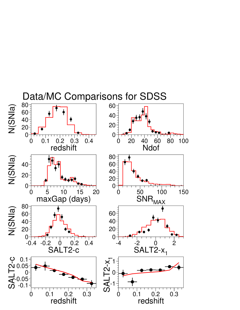
Figure 1.— Comparison of distributions for SDSS–II data (dots) and MC (histogram), where each MC distribution is scaled to have the same sample size as the data. The distributions are redshift, number of degrees of freedom in the salt-ii light curve fit, maximum rest-frame time difference (gap) between observations, maximum S/N, fitted salt-ii color ($c$) and stretch parameter ($x_{1}$). The bottom two panels show the mean fitted salt-ii color ($c$) and shape parameter ($x_{1}$) vs. redshift.

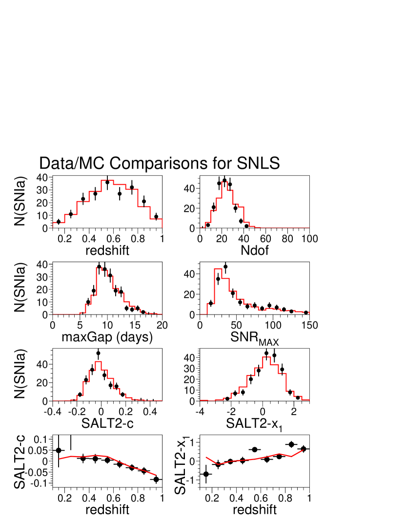
Figure 2.— Same as Figure 1, except for the SNLS3 sample.

3.1. Simulation of Noise

Since the three scatter-dependent variables (Hubble scatter, $B-V-c$ photo-$z$ precision) are sensitive to the flux uncertainties, it is important to accurately simulate these uncertainties. The simulation strategy is to first calculate the uncertainties from a model based on measurements of the sky level and PSF. To accurately check the model, the true uncertainty for each observation in the data is compared to the calculated model uncertainty. Discrepancies between the true and calculated uncertainties are corrected by fitting for ad-hoc parameters. The simulated uncertainty model in photoelectrons ($\sigma_{\rm SIM}$) is given by

$$\sigma_{\rm SIM}^{2}=F + (A\cdot b)+(qF)^{2}+(\sigma_{0}\cdot 10^{0.4\cdot{\rm ZPT}_{\rm pe}})^{2}$$ (4)

$$+ \sigma_{\rm HOST}^{2}$$

where $F$ is the flux, $A=[2\pi\int{\rm PSF}^{2}(r,\theta)rdr]^{-1}$ is the noise-equivalent area, $b$ is the effective sky level including dark current and readout noise, and $q$ and $\sigma_{0}$ are fitted ad-hoc parameters. ${\rm ZPT}_{\rm pe}$ is defined such that the number of CCD photoelectrons for a point source of magnitude $m$ is given by $10^{-0.4(m-{\rm ZPT}_{\rm pe})}$; thus the $\sigma_{0}$ term is independent of the PSF, sky level and host-galaxy. The quantity $\sigma_{\rm HOST}$ is simulated for the SDSS–II sample using a library of galaxies that have a spectroscopic redshift and a well measured profile consistent with either exponential or de Vaucouleurs.

To check the uncertainty calculation, $\sigma_{\rm SIM}$ is computed for each epoch in the data and compared to the measured uncertainty $\sigma_{\rm DATA}$. The left panels in Figure 3 show that the first two terms, $F+Ab$, are not adequate to reproduce the observations. The right panels in Figure 3 show that the fitted $\sigma_{0}$ term results in good agreement over a wide range of PSF values. A separate $\sigma_{0}$ value is evaluated for each filter and for each sample (Table 2). The quadratic term $q$ is sensitive to large flux values with ${\rm S/N}\sim 10^{2}$. The value of $q$ is obtained from minimizing $\chi^{2}=\sum_{s}[(\sigma_{\rm SIM}/\sigma_{\rm DATA})_{s}-1]^{2}$, where the sum ($s$) is over $\log_{10}({\rm S/N})$ bins; $q\simeq 0.01$ for the SDSS bands, and $q\sim 0.001$ for the SNLS bands. For SNLS, it is difficult to interpret this low value of $q$ because uncertainties on the SN flux (Poisson noise and flat-fielding noise) only arise via the normalization of errors based on the intra-night flux scatter.

Finally, note that the terms $F+(A\cdot b)+\sigma_{\rm HOST}^{2}$ are determined from observations and first principles, while $q$ and $\sigma_{0}$ are empirically determined parameters. The $q$ term corresponds to a zeropoint uncertainty. The $\sigma_{0}$ term is not understood, although this term works surprisingly well for both the SDSS–II and SNLS3 surveys even though the respective photometry codes are independent.

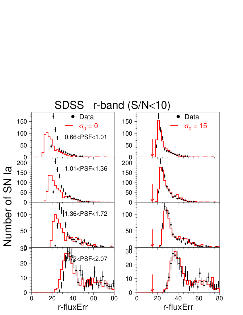
Figure 3.— Left panels show the $r$-band flux-uncertainty distribution for the data (black dots) and for the calculation (histogram), $\sigma_{\rm SIM}=\sqrt{F+Ab}$ with $\sigma_{0}=0$ and $q=0$. Each descending plot is for a different PSF range (FWHM, arcsec) as indicated on the plot. Right panels show the $\sigma_{\rm SIM}$ calculation including the best-fit $\sigma_{0}$ value labeled on the plot and shown by the arrow. The flux unit shown is that used for light curve fits (not photoelectrons).

Table 2 Fitted $\sigma_{0}$ values for SDSS–II and SNLS3.

	$10^{11}\times\sigma_{0}$ for
Filter	SDSS–II	SNLS3
$u$	28	—
$g$	10	0.22
$r$	15	0.30
$i$	23	1.08
$z$	63	1.62

3.2. Intrinsic-scatter Models

The intrinsic scatter models are summarized in Table 3. These models are defined as wavelength-dependent perturbations to the salt-ii spectral model, and these perturbations average to zero so that the underlying salt-ii model is not changed. All models are independent of redshift, and only the explosion models from KRW09 depend on epoch. We begin with the phenomenological functions (see “FUN” prefix) with parameters arbitrarily chosen to increase the scatter. The coherent model (FUN-COH) assigns a single magnitude shift for all wavelengths; for each SN this shift is given by a Gaussian-random number with $\sigma_{\rm COH}=0.13$ mag. The other two FUN functions are designed to probe a wider variety of wavelength-dependent scatter with a coherence length of a few hundred Å. First a sequence of nodes is defined at $1000$ Å intervals in the rest frame. An independent Gaussian random scatter is selected at each node with $\sigma_{\rm node}=\sigma_{5500}\exp[-(\lambda_{\rm node}-5500)/3000]$ so that there is more scatter at bluer wavelengths. The variation is the same at all epochs. A continuous function of wavelength is constructed by connecting the node values with sine functions so that the derivative is zero at each node. FUN-COLOR is defined with $\sigma_{5500}=0.06$ and is shown in Figure 4 for a few simulated SN. FUN-MIX is defined with $\sigma_{5500}=0.045$ along with a coherent term $\sigma_{\rm COH}=0.09$ mag.

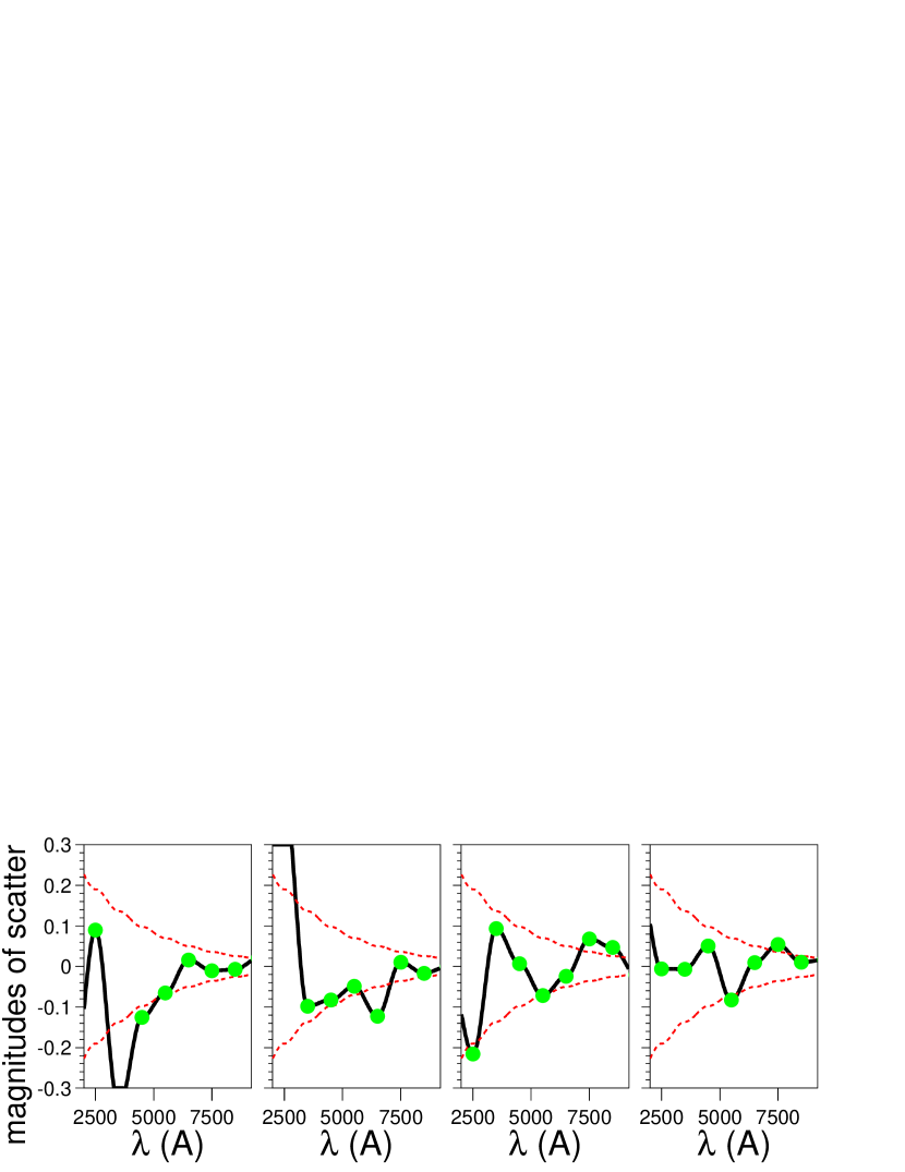
Figure 4.— Illustration of FUN-COLOR for four simulated SNe. Black lines show the $\lambda_{\rm rest}$-dependent variation. Solid dots show the Gaussian-random variations at the nodes, and dashed lines show $\pm 1~{}\sigma$ vs. $\lambda_{\rm rest}$.

Table 3 Summary of Intrinsic-scatter Models. $\lambda_{\rm rest}$ refers to rest-frame wavelength.

Model
Name	Description
NONE	Poisson noise only
FUN-COH	Coherent variation at all $\lambda_{\rm rest}$
	($\sigma_{\rm COH}=0.13$ mag)
FUN-COLOR	$\sigma_{\rm node}=0.06\exp[-(\lambda_{\rm node}-5500)/3000]$
	(Figure 4)
FUN-MIX	$\sigma_{\rm node}=0.045\exp[-(\lambda_{\rm node}-5500)/3000]$
	and $\sigma_{\rm COH}=0.09$
G10	$\sigma_{\rm COH}=0.09$ mag and $\sigma_{\rm node}$
	from solid curve in Figure 8 of G10
C11_0	$UBVRI$ correlation matrix. $\rho_{U^{\prime},U}=0$.
C11_1	Same for $UBVRI$, $\rho_{U^{\prime},U}=+1$.
C11_2	Same for $UBVRI$, $\rho_{U^{\prime},U}=-1$.
(KRW09 2D explosion models)
iso3_dc1	$N_{\rm ignit}=~{}60$, ${\rm Ka}_{\rm min}=1$
iso6_dc1	$N_{\rm ignit}=100$, ${\rm Ka}_{\rm min}=1$
iso6_dc2	$N_{\rm ignit}=100$, ${\rm Ka}_{\rm min}=250$
iso6_dc3	$N_{\rm ignit}=100$, ${\rm Ka}_{\rm min}=750$
iso6_dc4	$N_{\rm ignit}=100$, ${\rm Ka}_{\rm min}=1500$
iso6_dc5	$N_{\rm ignit}=100$, ${\rm Ka}_{\rm min}=2250$
iso8_dc3	$N_{\rm ignit}=150$, ${\rm Ka}_{\rm min}=750$
asym1_dc3	$N_{\rm ignit}=120$, ${\rm Ka}_{\rm min}=750$

The next two models (G10 and C11) are based on measurements from data combined with assumptions needed to create a model that is a continuous function of wavelength. The G10 error model was obtained as part of the salt-ii training process in which they minimized the likelihood of light curve amplitude residuals using a parametric function of central rest-frame wavelength, assuming uncorrelated residuals in different passbands. The resulting wavelength-dependent function (Figure 8 of G10) has approximate values of 0.07, 0.03, 0.02, 0.03, 0.06 mag at the $U,B,V,R,I$ central wavelengths, respectively. This function is not intended to represent a wavelength dependent scatter, but rather it is a model of independent broadband scatter as a function of central wavelength. To translate this broadband model into a wavelength model, independent random scatter values ($\sigma_{\rm node}$) are selected every 800 Å, and these node values are connected with the same sine-interpolation that is used for the phenomenological “FUN” functions. Since this procedure reduces the resulting broadband scatter, $\sigma_{\rm node}$ is multiplied by $1+(\lambda_{\rm rest}-2157)/9259$ so that the simulated $UBVRI$ broadband scatter matches the G10 function. In addition to a wavelength-dependent function, the G10 model includes a coherent term, $\sigma_{\rm COH}=0.09$ mag.

The model of Chotard (2011, hereafter C11); Chotard et al. (2011, hereafter C11) is based on a covariance scatter matrix among the $UBVRI$ filter passbands, and is derived from an analysis of spectral correlations using high quality spectra from the Supernova Factory (Aldering et al., 2002). The broadband covariance model is translated into a wavelength-dependent model as follows. First, the model is extrapolated to wavelengths below the $U$ band (3600 Å) by defining an ad-hoc $U^{\prime}$ filter with central wavelength $\bar{\lambda}_{\rm obs}=2500$ Å. The G10 scatter value of $\sigma_{\rm node}=0.59$ mag is used for $U^{\prime}$, and we model three different assumptions for the reduced correlation between $U^{\prime}$ and $U$: $\rho_{U^{\prime},U}=0$ (incoherent,C11_0), $\rho_{U^{\prime},U}=+1$ (C11_1), and $\rho_{U^{\prime},U}=-1$ (C11_2). For each simulated SN, six random magnitude shifts are selected according to the C11 correlation matrix in upper half of Table 4; these shifts are assigned to the central ${U^{\prime}}UBVRI$ wavelengths. A continuous function of wavelength is obtained by interpolating these six points with a sine function, similar to the FUN-COLOR interpolation in Figure 4. Finally, the scatter function is multiplied by 1.3 to compensate for the fact that the wavelength interpolation reduces the broadband covariances. The correlation matrix realized by the simulation is shown in bottom half of Table 4 for the C11_1 model. The realized correlation matrix is slightly different than the input model because the input model is described by broadband covariances, while the simulated model depends on wavelength. In principle a more finely tuned spectral model in the simulation would result in the exact C11 covariances, but we believe that the simple and approximate model used here is adequate, especially in light of the large and unknown uncertainties on the covariances.

Table 4 Reduced Correlation Matrix from the C11_1 Model and Realized from the Simulation

	$U^{\prime}$	$U$	$B$	$V$	$R$	$I$
	(From C11)
$U^{\prime}$	$+1.00$	$+1.00$	$-0.12$	$-0.77$	$-0.91$	$-0.22$
$U$	$+1.00$	$+1.00$	$-0.12$	$-0.77$	$-0.91$	$-0.22$
$B$	$-0.12$	$-0.12$	$+1.00$	$+0.57$	$-0.24$	$-0.89$
$V$	$-0.77$	$-0.77$	$+0.57$	$+1.00$	$+0.53$	$-0.40$
$R$	$-0.91$	$-0.91$	$-0.24$	$+0.53$	$+1.00$	$+0.49$
$I$	$-0.22$	$-0.22$	$-0.89$	$-0.40$	$+0.49$	$+1.00$
Diag	$0.59$	0.06	0.04	0.05	0.04	0.08
	(Realized in simulation)
$U^{\prime}$	$+1.00$	$+0.99$	$+0.12$	$-0.78$	$-0.96$	$-0.28$
$U$	$+0.99$	$+1.00$	$+0.20$	$-0.73$	$-0.96$	$-0.34$
$B$	$+0.12$	$+0.20$	$+1.00$	$+0.40$	$-0.27$	$-0.93$
$V$	$-0.78$	$-0.73$	$+0.40$	$+1.00$	$+0.72$	$-0.34$
$R$	$-0.96$	$-0.96$	$-0.27$	$+0.72$	$+1.00$	$+0.36$
$I$	$-0.28$	$-0.34$	$-0.93$	$-0.34$	$+0.36$	$+1.00$
Diag	$0.59$	0.073	0.036	0.051	0.042	0.083

The final class of brightness variations is based on 2D explosion models with random ignition points (KRW09), followed by radiative transfer calculations using the SEDONA program (Kasen et al., 2006). Isotropic models are obtained from ignition points that are randomly placed throughout the white dwarf (WD), while asymmetric models are obtained from ignition points within a cone whose apex is at the center of the WD. Both the isotropic and asymmetric models result in explosion asymmetries and a viewing angle dependence that contributes significantly to the intrinsic scatter. The width-luminosity relation is related to the number of ignition points ($N_{\rm ignit}$) because $N_{\rm ignit}$ affects the amount of pre-expansion before detonation, and hence the amount of ${}^{56}{\rm Ni}$ produced in the explosion. In a recent study by Blondin et al. (2011, hereafter B11), detailed comparisons between data and the KRW09 models were made. They conclude that the KRW09 models with the best spectroscopic agreement also have the best photometric agreement, and they identified a subset of eight models with the best agreement to data. Here we use these same eight models; they are shown in Table 3 along with a few parameters describing the number of ignition points and the detonation criteria. All of these models have an isotropic distribution of ignition points, and B11 note that radial fluctuations in isotropic models can lead to significant viewing angle asymmetries.

We initially used these KRW09 models in the SNANA simulation to generate light curves corresponding to the SDSS–II and SNLS3. While the data/MC comparisons are visually impressive, the simulated light curves are not adequate for this study because the salt-ii light curve fits are in general rather poor. This trend of poor light curve fits was also noted in B11.

Instead of attempting an absolute prediction with the KRW09 models, we have instead used these models as a perturbation on the salt-ii model. In short, the salt-ii model describes the stretch and color relations, while the KRW09 models are used to describe the intrinsic scatter. The spectral flux ($F$) is given by

$$F=F_{\rm SALT2}\times\frac{F_{\rm KRW09}({\rm random}~{}\cos\phi)}{F_{\rm KRW09}(\cos\phi=0)}$$ (5)

where $\phi$ is the viewing angle. The corresponding mag-shifts are illustrated in Figure 5 as a function of wavelength for a two extreme viewing angles.

Figure 5.— Magnitude shift applied to the salt-ii spectral model vs. wavelength for the KRW09 models. The solid and dashed curves reflect different viewing angles as indicated in the legend above the plots. The label on each panel indicates the specific explosion model as defined in Table 3.

4. Analysis

Here we describe the determination of the three scatter-dependent quantities used to evaluate models of intrinsic brightness variations. All analyses are based on light curve fits using the salt-ii model.

4.1. Review of salt-ii Model

The salt-ii SN Ia model flux is a function of wavelength ($\lambda$) and time ($t$) in the rest-frame,

$$F(t,\lambda)=x_{0}\left[M_{0}(t,\lambda)+x_{1}M_{1}(t,\lambda)\right]\times\exp[c\cdot{\rm CL}(\lambda)]$$ (6)

where the spectral sequences ($M_{0}$ and $M_{1}$) and color law (${\rm CL}(\lambda)$) are derived from the training in G10. Synthetic photometry in the observer frame is obtained by redshifting Eq. 6 and multiplying by the filter response and Galactic transmission. The overall scale ($x_{0}$), stretch ($x_{1}$), color ($c$) and time of peak brightness ($t_{0}$) are determined for each SN in a light curve fit that minimizes a $\chi^{2}$ based on the difference between the data and synthetic photometry. Eq. 6 is valid for $2000<\lambda<9200$ Å, and the model is valid for observer-frame filters that satisfy

$$2800<\bar{\lambda}_{\rm obs}/(1+z)<7000~{}~{}{\rm\AA},$$ (7)

where $\bar{\lambda}_{\rm obs}$ is the central wavelength of the filter.

An effective $B$-band magnitude is defined to be $m_{B}=-2.5\log_{10}(x_{0})+10.635$; this is the observed magnitude through an idealized filter that corresponds to the $B$ band in the rest-frame of the SN. The fitted distance modulus is given by

$$\mu_{\rm fit}=m_{B}-M+\alpha x_{1}-\beta c$$ (8)

where $\alpha$, $\beta$ and $M$ are determined from a global fit to all of the SNe using the “SALT2mu” program described in M11 and below in Section 6.

4.2. Hubble Scatter

The well known Hubble scatter is defined as the dispersion on $\Delta\mu$, the difference between the fitted (measured) distance modulus and the distance modulus calculated from the best-fit cosmological parameters. To simplify the analysis here we do not fit for the $\alpha$ and $\beta$ parameters, nor do we fit for the best-fit cosmological parameters. Instead we compute the dispersion of

$$\Delta\mu\equiv\mu_{\rm fit}({\rm Eq.}\ref{eq:muSALT2})-\mu_{\rm calc}(z,\Omega_{\rm M},\Omega_{\Lambda},w)$$ (9)

where $\alpha=0.11$, $\beta=3.2$, $M=-19.36$ ($H_{0}=70$ km s^-1 Mpc^-1 ), and $\mu_{\rm calc}$ is the calculated distance modulus assuming a $\Lambda{\rm CDM}$ cosmology with $w=-1$, $\Omega_{\rm M}=0.3$, $\Omega_{\Lambda}=0.7$. Although the fitted $\alpha$ and $\beta$ may have given slightly different $\Delta\mu$ values, the resulting bias is more than an order of magnitude smaller than the dispersion, and hence the impact of this approximation is negligible.

4.3. Color Precision

The color precision test compares the fitted salt-ii color ($c$) to the true $B-V$ rest-frame color at the epoch of peak brightness. Since the fitted color is really a color excess, $c=E(B-V)$, and the color also depends slightly on the stretch, the true $B-V$ color does not exactly correspond to $c$. A numerical examination of the model shows that with no intrinsic scatter,

$$B-V=c^{\prime}=(1.016\times c)+(x_{1}/1250)+0.0232$$ (10)

and therefore we examine the dispersion on $B-V-c^{\prime}$. The dispersion on $c-c^{\prime}$ is $\sim 0.001$, more than an order of magnitude smaller than the dispersion on $B-V-c^{\prime}$, and thus this correction has little effect. The evaluation of $c^{\prime}$ is from simply plugging the fitted $c$ and $x_{1}$ values into Eq. 10. The naive rest-frame magnitudes $M^{\star}_{B}$ and $M^{\star}_{V}$ are obtained from Eq. 6 using the best-fit parameters ($c$, $x_{0}$, $x_{1}$) and using the $B$ and $V$ filter-transmission functions. However, these naive magnitudes are not necessarily the true values if there are intrinsic color variations. To obtain a better approximation for the magnitudes we fit only the two nearest observer-frame bands that bracket the $B$ or $V$ band in wavelength.

The details of the fitting procedure are as follows. First a normal fit is done using all filters to determine the fit parameters ($t_{0}$,$c$,$x_{0}$, $x_{1}$). For each rest-frame band one additional fit is performed using only the two nearest observer-frame bands and holding $t_{0}$ and $x_{1}$ fixed from the normal fit. The floated color ($c$) and distance ($x_{0}$) parameters provide the flexibility to fit both observer-frame bands regardless of how much intrinsic color variation exists. The two-band fit parameters are $c^{B},x_{0}^{B}$ for the $B$ band, and $c^{V},x_{0}^{V}$ for the $V$ band. After finishing both two-band fits the $B-V$ color is computed as

$$B-V = {M^{\star}}(T_{B},~{}t_{0},~{}x_{1}=0,~{}c^{B},~{}x_{0}^{B})$$ (11)

$$- {M^{\star}}(T_{V},~{}t_{0},~{}x_{1}=0,~{}c^{V},~{}x_{0}^{V})$$

where $M^{\star}$ is the magnitude computed from Eq. 6 using filter-transmission functions $T_{B,V}$, and with $x_{1}=0$ so that all $B-V$ colors correspond to an SN Ia with the same stretch.

This fitting procedure was tested on an SNLS3 simulation in which the maximum S/N was artificially set to 1000 for every SN regardless of redshift. The rms on $B-V-c^{\prime}$ is 0.002 mag, an order of magnitude smaller than the observed dispersion.

4.4. Photo-$z$ Precision

The photo-$z$ precision is based on the difference between the SN redshift determined from broad band photometry and the more precise spectroscopic redshift. The basic photo-$z$ method is to extend the usual methods of fitting light curves to include the redshift as a fifth fit parameter. Particular attention is needed to estimate initial parameter values near those corresponding to the global minimum-$\chi^{2}$, and to iteratively determine which filters satisfy Eq. 7. Details of the photo-$z$ fitting process are given in K10.

There are two modifications in our photo-$z$ fitting procedure compared to K10. The first change is that we use the known spectroscopic redshift as the initial estimate in order to reduce catastrophic outliers. The fitting task has thus been changed to find a local photo-$z$ minimum near the true redshift instead of searching the entire redshift range for a global minimum. The second change is related to estimating the initial parameter $x_{0}$ for each color value along the coarse-grid search in color. In K10, $x_{0}$ at each grid point was calculated using the current color, photo-$z$ and a reference cosmology. Here we analytically minimize for $x_{0}$, making the fitted photo-$z$ less sensitive to the absolute brightness. To check that the fitted photo-$z$ depends only on the SN colors we have applied this method to simulations with no intrinsic scatter and with the coherent scatter model (see COH entry in Table 3); the photo-$z$ precision is the same in both cases.

4.5. Statistics Summary

After applying the selection requirements in Section 2, along with the light curve fitting requirements for each dispersion variable, the number of SNe Ia for each sample and for each dispersion variable is shown in Table 5

The smaller photo-$z$ samples arise from a light curve fitting requirement. For each successive fit iteration, observer-frame filters are added or dropped based on which filters satisfy the salt-ii wavelength range in Eq. 7 with $z=$ photo-$z$. If any filter fails this wavelength requirement after the last fit iteration, the SN is rejected; this requirement avoids fitting to wavelength regions in which the salt-ii model may be poorly defined.

The smaller SNLS3 sample for the $B-V-c^{\prime}$ analysis is due to SNe Ia at $z>0.7$; for these objects the observer-frame $i$ and $z$ bands no longer bound the rest-frame $V$ band.

Table 5 Number of SNe Ia After Selection Requirements.

	Number of SNe Ia for:
Survey	Hubble Resid	$B-V-c^{\prime}$	Photo-$z$
SDSS–II	251	245	208
SNLS3	191	120	176

4.6. Quantifying the Dispersions

The data and MC dispersions are measured from the following variables,

$$\Delta_{\mu} \equiv (\mu_{\rm fit}-\mu_{\rm calc})/(1+z)$$

$$\Delta_{c} \equiv (B-V-c^{\prime})/(1+z)$$

$$\Delta_{z} \equiv (Z_{\rm phot}-Z_{\rm spec})/(1+z)$$ (12)

where the $(1+z)^{-1}$ factor is included to reduce the redshift-dependent variation from measurement uncertainties. These three quantities are shown in Figure 6 for the data and MC, and for both the SDSS–II and SNLS3 samples. The MC includes only Poisson noise (no intrinsic variation), and hence the data-MC difference in the width illustrates the size of the intrinsic component that is needed. The $\Delta_{\mu}$ comparison shows the most obvious discrepancy. The $\Delta_{z}$ and $\Delta_{c}$ discrepancies are more subtle, indicating that the effect of color variations is smaller than the coherent variation.

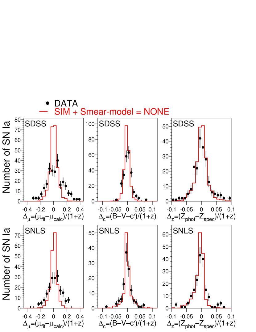
Figure 6.— Comparison of $\Delta_{\mu}$, $\Delta_{c}$ and $\Delta_{z}$ distributions for data (dots) and MC (histogram). The upper plots are for the SDSS–II and lower plots are for SNLS3. The MC includes Poisson noise but no intrinsic brightness variation, and each MC distribution is scaled to have the same sample size as the data.

To quantify the dispersions we compute the median, $M_{\Delta}\equiv{\rm median}|\Delta_{x}|$, where $x=\mu,z,c$ indicates the variable type. In particular, we compute the MC/data ratio of medians,

$$R_{\rm MC/Data}={M_{\Delta}^{\rm MC}}/{M_{\Delta}^{\rm Data}}~{}.$$ (13)

With the correct model of brightness variations we expect $R_{\rm MC/Data}=1$ for all three variables and for both surveys.

The uncertainty on the median is calculated as follows. For $N$ SNe, the statistical uncertainty on $N/2$ is $\sigma_{(N/2)}=\sqrt{N}/2$. The median uncertainty ($\sigma_{M}$) is defined such that $N-\sigma_{(N/2)}$ values of $|\Delta_{x}|$ lie below $M-\sigma_{M}^{-}$ and $N+\sigma_{(N/2)}$ values lie below $M+\sigma_{M}^{+}$. For a rapidly falling distribution we typically find that $\sigma_{M}^{+}>\sigma_{M}^{-}$. Here we define a symmetric uncertainty, $\sigma_{M}\equiv(\sigma_{M}^{-}+\sigma_{M}^{+})/2$.

As a numerical crosscheck we analyze SDSS–II simulations in which the exposure time is adjusted for each SN so that the maximum S/N is $10^{4}$. The resulting dispersions, defined simply as a Gaussian fitted $\sigma$, are $0.0003$, $0.002$, and $0.001$ mag for the three variables (Eq. 12), respectively; these dispersions are more than an order of magnitude smaller than the dispersions observed in the data.

5. Results

The MC/data ratio of medians, $R_{\rm MC/Data}$ (Eq. 13), is shown in Figure 7 for all of the models in Table 3, and for both surveys. With no model of intrinsic scatter, $R_{\rm MC/Data}$ is well below unity in all cases. Adding a coherent scatter (FUN-COH) predicts the Hubble dispersion ($\Delta_{\mu}$), but has no impact on the color and photo-$z$ dispersion. The FUN-COLOR model almost predicts the Hubble dispersion, but may overestimate the color precision. FUN-MIX has been artificially tuned to predict the dispersion in all quantities, although the photo-$z$ dispersion may still be underestimated. The G10, C11_0 and C11_1 models provide decent predictions, with a slight underestimate in the photo-$z$ dispersion. The C11_2 model underestimates the Hubble dispersion. Recall that the G10 model includes only positive correlations, mainly from the coherent term $\sigma_{\rm COH}=0.09$, while the C11 model includes both positive and negative correlations. This G10 versus C11 comparison illustrates that there can be significant degeneracies among models of intrinsic brightness variations. The KRW09 models give a poorer description of the dispersion because the Hubble dispersion is always underestimated.

Figure 7.— $R_{\rm MC/Data}$ for $\Delta_{\mu,z,c}$ as indicated in the legend panel. Solid-filled symbols are for the SDSS–II and open symbols are for SNLS3. The intrinsic variation model for the simulation is indicated at the top of each panel.

5.1. Systematics Tests

Here we describe some systematics tests to demonstrate the robustness of the results in Figure 7. We use the FUN-COH scatter model as the reference simulation for these tests which are summarized in Figure 8. For each test a change is applied to the simulation and then analyzed in exactly the same manner.

Figure 8.— $R_{\rm MC/Data}$ for $\Delta_{\mu,z,c}$ as indicated in the legend panel from Figure 7. The first panel is for the FUN-COH scatter model using the nominal simulation. The systematic test indicated above each panel is applied to the simulation using the same FUN-COH scatter model. The horizontal dashed lines are the same in each panel, and are intended to guide the eye.

The first test is based on the precision in the flux uncertainties in the data. For pre-explosion epochs in which the true SN flux is known to be zero, examining the S/N distribution shows that the uncertainties are accurate to within 5%. The test labeled $\sigma_{\rm SIM}\times 1.05$ corresponds to a simulation with 5% larger uncertainties on all of the fluxes.

The next set of tests is based on a 0.02 mag zeropoint change in each filter ($\delta{\rm ZPT}_{griz}$). Note that this change is two times larger than the uncertainty reported by each survey team.

Uncertainties on the Galactic extinction are examined by first increasing the estimated 16% scatter to 24% ($\times 1.5$ MW-Gal), and then increasing the reddening parameter by 10%, to $R_{V}=3.4$.

The next test is based on changing $\beta$ from 3.2 to 2.5, a $5\sigma$ change from G10.

The next two tests are based on changing the population parameters for $x_{1}$ and $c$ (Table 1). The simulated $x_{1}$ population is shifted toward faster-declining light curves by setting $\sigma_{+}=0.5$ and $\sigma_{-}=1.8$ (compare to nominal parameters in Table 1). The simulated color population is shifted toward the red by setting $\sigma_{+}=0.18$ and $\sigma_{-}=0.05$. For these systematic tests, the resulting data/MC comparisons for stretch and color are shown in Figure 9; the data and MC are clearly discrepant.

For all of these systematic tests, $R_{\rm MC/Data}$ remains significantly below unity for the $B-V-c^{\prime}$ and photo-$z$ variables. We also note that the independent SDSS–II and SNLS3 results are consistent, showing consistency over different redshift ranges.

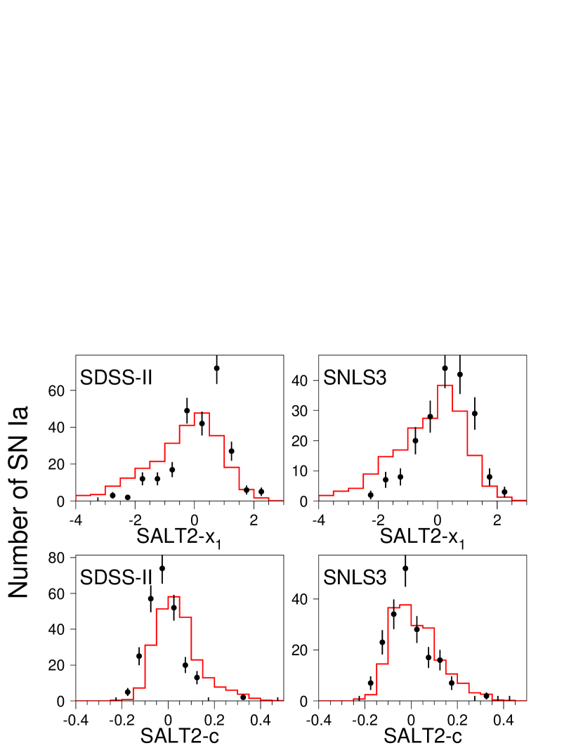
Figure 9.— Comparison of fitted stretch ($x_{1}$) and color ($c$) distributions for data (dots) and modified MC (histogram), where each MC distribution is scaled to have the same statistics as the data. The simulated populations have been modified for systematic tests explained in the text.

6. Impact of Intrinsic Scatter Model on the Hubble Diagram

Here we investigate the potential Hubble diagram bias from using an incorrect model of intrinsic scatter. We use four intrinsic scatter models that give reasonable data/MC agreement in Figure 7: FUN-MIX, G10, C11_0 and C11_1. Recall that data/MC agreement in these dispersion variables means that the intrinsic scatter model cannot be ruled out, but the agreement does not ensure that the underlying model is correct.

The Hubble bias is determined from the difference between an ideal analysis using the correct intrinsic scatter matrix (Section 6.1), and a conventional analysis that adds a wavelength-independent scatter to bring the reduced $\chi^{2}$ to unity (Section 6.2). The ideal analysis is based on simulations with the correct model of intrinsic scatter, and thus does not reflect a realistic analysis that could be applied to data. The conventional analysis, however, reflects a realistic analysis that has often been applied to data. In Section 6.3 the Hubble bias is translated into a bias on the dark energy equation of state parameter $w$, and in Section 6.4 the biases are reevaluated with Malmquist bias corrections.

6.1. Determining the Intrinsic-scatter Matrix

To evaluate the effect of intrinsic scatter in the analysis of cosmological parameters, we first need to briefly summarize the concept of an intrinsic scatter matrix introduced in Section 2 of M11. Cosmology fitters in general minimize the function

$$\chi^{2}=\sum_{i}{\Delta\mu}_{i}/({\sigma_{{\rm stat},i}}^{2}+{\sigma_{{\rm int},i}}^{2})$$ (14)

where $\Delta\mu_{i}$ is the difference between the fitted and calculated distance modulus (Eq. 9) for the $ith$ SN, $\sigma_{{\rm stat},i}$ is the statistical (fitted) error on $\Delta\mu_{i}$, and $\sigma_{{\rm int},i}$ is an ad hoc parameter defined so that $\chi^{2}/N_{\rm dof}=1$. Since $\sigma_{{\rm stat},i}$ is computed from a statistical correlation matrix between the salt-ii fit parameters ($m_{B},x_{1},c$), M11 proposed an analogous “intrinsic-scatter covariance matrix” (denoted $\Sigma$) to compute $\sigma_{\rm int}$. Dropping the SN index $i$, the ad-hoc error term is

$$\sigma_{\rm int}^{2} = \Sigma_{00}+\alpha^{2}\Sigma_{11}+\beta^{2}\Sigma_{cc}$$ (15)

$$+ 2\alpha\Sigma_{01}-2\beta\Sigma_{0c}-2\alpha\beta\Sigma_{1c}~{}~{},$$

where the subscript correspondence is $0,1,c\to m_{B},x_{1},c$, $\sqrt{\Sigma_{00}}\equiv\sigma_{m_{B}}^{\rm int}$, $\sqrt{\Sigma_{11}}\equiv\sigma_{x1}^{\rm int}$, and $\sqrt{\Sigma_{cc}}\equiv\sigma_{c}^{\rm int}$. All SNIa-cosmology analyses to date have used the simplifying assumption that $\sigma_{\rm int}=\sigma_{m_{B}}^{\rm int}=\sqrt{\Sigma_{00}}$, and ignored the other $\Sigma$ terms in Eq. 15. We refer to this method as the “$m_{B}$-only” method, while the $\Sigma$-fit method refers to using additional terms in Eq. 15. The $m_{B}$-only method is valid if the intrinsic scatter is independent of wavelength, or if $\sigma_{{\rm stat},i}$ from the light curve fit includes the wavelength dependence of the scatter. The FUN-COH panel in in Figure 7 clearly shows that the intrinsic scatter cannot be constant (i.e., wavelength independent). M11 noted that using the $m_{B}$-only method can lead to biased values of $\alpha$ and $\beta$. Here we go a step further and examine biases in simulated Hubble diagrams.

Since we do not have reliable methods for determining $\Sigma$ from the data, we determine $\Sigma$ from an artificial analysis using a simulation with the correct model of intrinsic scatter but without Poisson fluctuations from the calculated measurement uncertainties (Eq. 4); therefore the only source of scatter is from intrinsic variations. Although Poisson fluctuations are not applied, the uncertainties are included in the light curve fit-$\chi^{2}$ calculations so that the correct filter-dependent weights are used. For example, the SDSS $u$ band has relatively poor S/N compared to the other bands and therefore this passband has less weight in determining $\Sigma$. We refer to these simulations as “intrinsic-only” to distinguish them from the “nominal” simulations that include Poisson fluctuations. This intrinsic-only simulation is illustrated in Figure 10 for the special case with no intrinsic scatter; the simulated fluxes lie exactly on the best-fit salt-ii model and they have the correct uncertainties corresponding to real observations.

To better compare the resulting bias to the uncertainty reported in Sullivan et al. (2011), the simulations have been adjusted to better match the data sample used in this SNLS3 analysis. First, the SDSS–II sample size is reduced by a factor of three to correspond to the first-season sample used in the SNLS3 analysis. The next change is that the S/N requirement in the three passbands (see end of Section 2) is relaxed from 8 to 5. Finally, we have included a simulated nearby ($z<0.1$) sample as explained in the Appendix. To measure biases with good precision, the MC sample sizes correspond to $20$ times the data statistics.

After performing salt-ii light curve fits on the simulated intrinsic-only sample, we define $\Delta_{m_{B}}^{\rm SIM}\equiv m_{B}({\rm fit})-m_{B}({\rm true})$ and $\Delta_{c}^{\rm SIM}\equiv c({\rm fit})-c({\rm true})$, where “true” indicates the true value from the simulation and “fit” indicates the result from a light curve fit. The true values are defined by the underlying salt-ii model before the intrinsic smearing model is applied. The covariance terms with the stretch parameter $x_{1}$ are negligible because the intrinsic scatter models are epoch-independent and thus do not change the light curve shape; the $x_{1}$-terms in $\Sigma$ are therefore ignored.

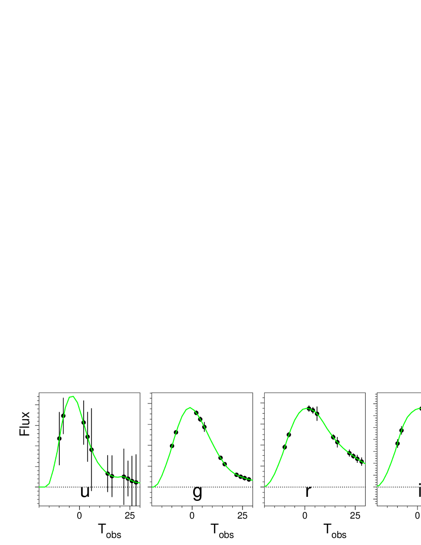
Figure 10.— Simulated SDSS–II light curve (solid dots) with no Poisson noise and no intrinsic scatter. Each curve is the best-fit salt-ii model.

The $2\times 2$ intrinsic scatter matrix is defined to be

$$\sqrt{{\Sigma}_{00}} = \sigma_{m_{B}}^{\rm int}={\rm rms}|\Delta_{m_{B}}^{\rm SIM}|$$

$$\sqrt{{\Sigma}_{cc}} = \sigma_{c}^{\rm int}={\rm rms}|\Delta_{c}^{\rm SIM}|$$

$${\Sigma}_{0c} = \langle\Delta_{m_{B}}^{\rm SIM}\Delta_{c}^{\rm SIM}\rangle~{}~{},$$ (16)

where $\langle\rangle$ indicates the mean value of the enclosed quantity. Another caveat is that $\Sigma$ depends on the redshift and on which filters are included in the light curve fit. This dependence is linked to the salt-ii color parameter ($c$) that is evaluated by extrapolating a color law to the central wavelengths of the $B$ and $V$ passbands. To address this caveat, $\Sigma$ is evaluated as a function of redshift and sample as shown in Figure 11. A second-order polynomial function of redshift is adequate to describe the components of $\Sigma$. For the FUN-MIX and G10 models, $\sigma_{m_{B}}^{\rm int}$ and $\beta\sigma_{c}^{\rm int}$ give a comparable contribution ($\sim 0.1$) to $\sigma_{\rm int}$. For the C11 models, $\sigma_{m_{B}}^{\rm int}\sim 0.03$ is much smaller than the contribution from $\beta\sigma_{c}^{\rm int}$.

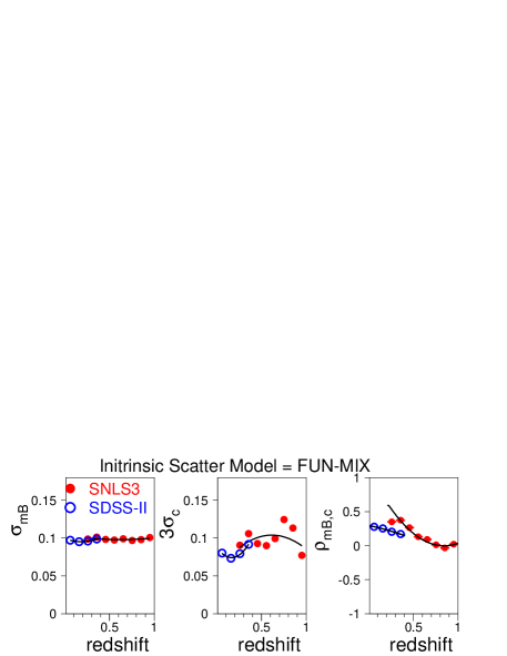
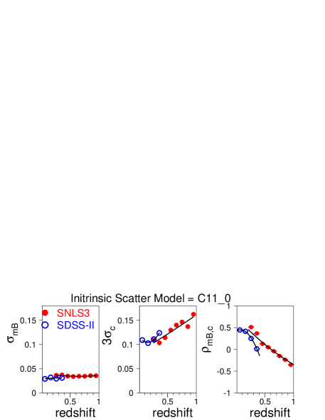
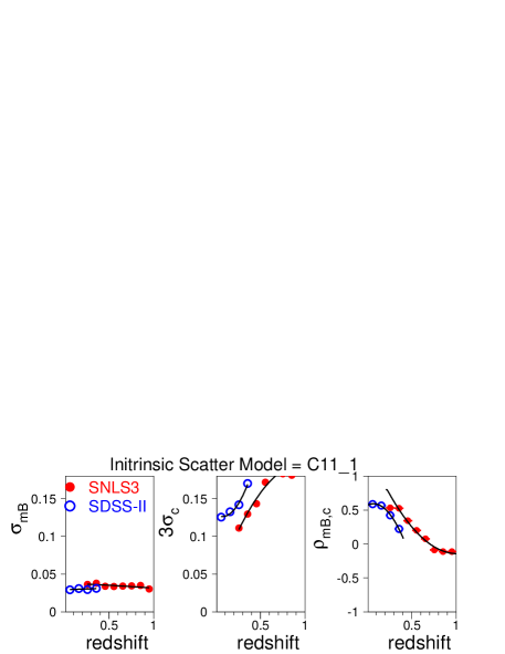
Figure 11.— Elements of intrinsic scatter matrix ($\Sigma$ ) for the simulated models indicated above each set of plots. The panels show the following parameters vs. redshift: $\sigma_{m_{B}}=\sqrt{\Sigma_{00}}$ (left), $3\sigma_{c}=3\sqrt{\Sigma_{cc}}$ (middle), and $\rho_{m_{B},c}=\Sigma_{0c}/(\sigma_{m_{B}}\sigma_{c})$ (right). The “int” superscripts have been dropped for clarity. Note that $\sigma_{m_{B}}$ and $3\sigma_{c}$ are in roughly the same units as the scatter in the distance modulus residual. The simulated SNLS3 (SDSS–II) samples are indicated by solid (open) circles. Each solid curves represents a second-order polynomial function of redshift used to describe $\Sigma$.

6.2. Fitting for $\alpha$, $\beta$, and the Distance Moduli

Using the fitted salt-ii parameters and uncertainties from the nominal MC, we use the SALT2mu program (M11) to minimize Eq. 14. This minimization gives the best-fit values of $\alpha$ and $\beta$, along with an independent offset ($M_{z}$) in each 0.1-wide redshift bin (Eq. 8). The separate offsets are used to eliminate the $\mu$-dependence on cosmological parameters. These fitted parameters are used to compute a distance modulus for each SN, and the resulting redshift+distance pairs form a Hubble diagram that can be fit for cosmological parameters. To properly evaluate the fit $\chi^{2}$ using the scatter matrix $\Sigma$, the light curve fits have been done with the salt-ii model uncertainties set to zero (hence reducing $\sigma_{{\rm stat},i}$) because they are now included in the SALT2mu fit as part of the $\sigma_{\rm int}$ calculation. This modification only affects the SALT2mu $\chi^{2}$ and has a negligible impact on the fitted parameters.

The $m_{B}$-only fit is based on the traditional method of tuning $\sigma_{m_{B}}^{\rm int}$ such that $\chi^{2}/N_{\rm dof}=1$, while setting all of the other covariance terms to zero. The light curve fits include the salt-ii model errors, and hence the intrinsic uncertainties corresponding to the G10 model are included. We note that there is an improved statistical treatment in March et al. (2011), using a Bayesian hierarchical model. While they obtain an uncertainty on $\sigma_{m_{B}}^{\rm int}$, their scatter model is fundamentally the same as our $m_{B}$-only model because they do not include additional covariance terms.

The SALT2mu fit results for both intrinsic scatter methods ($m_{B}$-only and $\Sigma$) are shown in Table 6.2. For both methods the fitted values of $\alpha$ agree well with the simulated input, $\alpha_{\rm SIM}=0.11$. For the FUN-MIX and G10 scatter models, the fitted values of $\beta$ agree well with the simulated input ($\beta_{\rm SIM}=3.2$) for both methods. For the C11 models, however, the situation is quite different. The $m_{B}$-only fitted $\beta$ values are too low by 0.3–0.6, and the significance of this bias ranges from 6 to 15 standard deviations. The $\Sigma$-fit $\beta$ values are consistent with $\beta_{\rm SIM}$.

Table 6 $\alpha$ and $\beta$ Fit Results from Simulations with Different Intrinsic-scatter Models, and $w$-bias Results from Cosmology Fits

Simulated	Intrinsic						Malmquist-
Scatter	Scatter		Fitted	Fitted		Uncorrected	Corrected
Model	Matrix	$\chi^{2}/N_{\rm dof}$	$\alpha$	$\beta$	$\beta$-bias	$w$-bias	$w$-bias
	SDSS-II
FUN-MIX	$\sigma_{m_{B}}^{\rm int}=0.087$	1.004	$0.114\pm 0.003$	$3.25\pm 0.04$	$-0.01\pm 0.01$	$+0.007\pm 0.006$	$-0.022\pm 0.005$
G10	$\sigma_{m_{B}}^{\rm int}=0.085$	0.993	$0.109\pm 0.003$	$3.20\pm 0.03$	$+0.04\pm 0.01$	$-0.002\pm 0.006$	$+0.011\pm 0.007$
C11_0	$\sigma_{m_{B}}^{\rm int}=0.082$	0.980	$0.117\pm 0.003$	$2.94\pm 0.03$	$-0.27\pm 0.02$	$+0.070\pm 0.009$	$-0.023\pm 0.008$
C11_1	$\sigma_{m_{B}}^{\rm int}=0.106$	0.985	$0.117\pm 0.003$	$2.72\pm 0.03$	$-0.50\pm 0.03$	$+0.109\pm 0.013$	$+0.011\pm 0.011$
FUN-MIX	$\Sigma$	1.038	$0.109\pm 0.003$	$3.25\pm 0.04$	—	—	—
G10	$\Sigma$	1.085	$0.106\pm 0.003$	$3.17\pm 0.03$	—	—	—
C11_0	$\Sigma$	1.076	$0.112\pm 0.003$	$3.21\pm 0.03$	—	—	—
C11_1	$\Sigma$	1.009	$0.110\pm 0.004$	$3.20\pm 0.04$	—	—	—
	SNLS3
FUN-MIX	$\sigma_{m_{B}}^{\rm int}=0.087$	0.980	$0.114\pm 0.002$	$3.17\pm 0.02$	$-0.04\pm 0.02$	$-0.011\pm 0.008$	$+0.012\pm 0.008$
G10	$\sigma_{m_{B}}^{\rm int}=0.069$	1.009	$0.112\pm 0.002$	$3.22\pm 0.02$	$+0.11\pm 0.01$	$-0.017\pm 0.011$	$+0.002\pm 0.011$
C11_0	$\sigma_{m_{B}}^{\rm int}=0.094$	0.998	$0.109\pm 0.002$	$2.86\pm 0.02$	$-0.31\pm 0.01$	$+0.072\pm 0.009$	$+0.001\pm 0.009$
C11_1	$\sigma_{m_{B}}^{\rm int}=0.127$	0.989	$0.108\pm 0.003$	$2.55\pm 0.02$	$-0.65\pm 0.02$	$+0.127\pm 0.012$	$+0.060\pm 0.011$
FUN-MIX	$\Sigma$	1.143	$0.104\pm 0.002$	$3.20\pm 0.02$	—	—	—
G10	$\Sigma$	1.207	$0.103\pm 0.002$	$3.12\pm 0.02$	—	—	—
C11_0	$\Sigma$	1.302	$0.104\pm 0.002$	$3.16\pm 0.02$	—	—	—
C11_1	$\Sigma$	1.297	$0.105\pm 0.003$	$3.20\pm 0.03$	—	—	—
	SDSS-II + SNLS3
FUN-MIX	$\sigma_{m_{B}}^{\rm int}=0.086$	0.991	$0.114\pm 0.002$	$3.20\pm 0.02$	$-0.02\pm 0.01$	$-0.019\pm 0.006$	$+0.010\pm 0.006$
G10	$\sigma_{m_{B}}^{\rm int}=0.075$	0.997	$0.112\pm 0.002$	$3.22\pm 0.02$	$+0.07\pm 0.01$	$-0.003\pm 0.005$	$-0.001\pm 0.005$
C11_0	$\sigma_{m_{B}}^{\rm int}=0.088$	1.007	$0.112\pm 0.002$	$2.89\pm 0.02$	$-0.26\pm 0.01$	$+0.035\pm 0.004$	$+0.018\pm 0.004$
C11_1	$\sigma_{m_{B}}^{\rm int}=0.119$	0.998	$0.111\pm 0.002$	$2.63\pm 0.02$	$-0.56\pm 0.02$	$+0.069\pm 0.010$	$+0.040\pm 0.011$
FUN-MIX	$\Sigma$	1.130	$0.105\pm 0.002$	$3.22\pm 0.02$	—	—	—
G10	$\Sigma$	1.177	$0.104\pm 0.002$	$3.15\pm 0.02$	—	—	—
C11_0	$\Sigma$	1.241	$0.107\pm 0.002$	$3.15\pm 0.02$	—	—	—
C11_1	$\Sigma$	1.267	$0.108\pm 0.002$	$3.20\pm 0.02$	—	—	—
	Nearby + SDSS-II + SNLS3
FUN-MIX	$\sigma_{m_{B}}^{\rm int}=0.085$	1.003	$0.115\pm 0.002$	$3.18\pm 0.02$	$-0.06\pm 0.01$	$-0.013\pm 0.003$	$-0.002\pm 0.003$
G10	$\sigma_{m_{B}}^{\rm int}=0.072$	1.010	$0.112\pm 0.001$	$3.23\pm 0.02$	$+0.07\pm 0.01$	$-0.001\pm 0.003$	$+0.001\pm 0.003$
C11_0	$\sigma_{m_{B}}^{\rm int}=0.086$	0.990	$0.113\pm 0.001$	$2.86\pm 0.01$	$-0.28\pm 0.01$	$+0.013\pm 0.003$	$-0.017\pm 0.003$
C11_1	$\sigma_{m_{B}}^{\rm int}=0.108$	0.998	$0.111\pm 0.002$	$2.68\pm 0.02$	$-0.48\pm 0.01$	$+0.020\pm 0.003$	$-0.006\pm 0.003$
FUN-MIX	$\Sigma$	1.077	$0.108\pm 0.001$	$3.23\pm 0.02$	—	—	—
G10	$\Sigma$	1.104	$0.105\pm 0.001$	$3.16\pm 0.01$	—	—	—
C11_0	$\Sigma$	1.127	$0.109\pm 0.001$	$3.15\pm 0.02$	—	—	—
C11_1	$\Sigma$	1.145	$0.108\pm 0.002$	$3.17\pm 0.02$	—	—	—

The reduced $\chi^{2}$ values are close to unity for the $m_{B}$-only method because of the explicit $\sigma_{m_{B}}^{\rm int}$ tuning. However, there is no such tuning for the $\Sigma$-fit method and the reduced $\chi^{2}$ are within about 10%–20% of unity. In summary, using the correct intrinsic scatter matrix $\Sigma$ in the SALT2mu fit results in unbiased $\beta$ values, and $\chi^{2}/N_{\rm dof}\simeq 1$. Using the simplistic $m_{B}$-only method results in a significant bias on $\beta$ for the C11 models.

Since the $\Sigma$-fit method results in unbiased $\beta$ values we define the $\mu$-bias to be $\Delta\mu=\mu_{mB{\rm-only}}-\mu_{\Sigma}$: $\mu_{\Sigma}$ is the distance modulus from the $\Sigma$-fit method and $\mu_{mB{\rm-only}}$ is the distance from the $m_{B}$-only method. Figure 12 displays $\Delta\mu$ versus redshift for each scatter model. For the FUN-MIX and G10 scatter models, the maximum $\Delta\mu$ variation is only $\sim 0.01$ mag over the redshift range of each survey. For the C11 models $\Delta\mu$ varies by several hundredths over the redshift range of each survey. This $\mu$-bias is caused by the bias in $\beta$ combined with Malmquist bias that results in bluer SN with increasing redshift. Figure 13 shows the mean fitted color value versus redshift, and the corresponding $\mu$-bias is $\Delta\mu\simeq\Delta\beta\times\langle c^{\rm fit}\rangle$ where $\Delta\beta$ is the bias in $\beta$ and $\langle c^{\rm fit}\rangle$ is the mean salt-ii color. The redshift dependence on $\Delta\mu$ is therefore directly proportional to the redshift dependence of $\langle c^{\rm fit}\rangle$. Figure 13 also shows the mean fitted stretch parameter ($x_{1}$) versus redshift. However, since the corresponding bias on $\alpha$ is less than $0.01$, the resulting $\mu$-bias is less than $0.01\times 0.3\sim 0.003$, and is thus much smaller than the bias from the color term.

To summarize, these bias tests show that the G10 model is internally consistent and that the wavelength dependence of the intrinsic scatter can be described with both methods. In the first method the scatter is described by the uncertainties in the salt-ii light curve fitting model, and the $m_{B}$-only scatter matrix is used in the SALT2mu stage. In the second $\Sigma$-fit method the light curve fitting model uncertainties are set to zero and the full intrinsic scatter matrix is used in the SALT2mu fitting stage. The difference in results between these two methods, as applied to simulations based on the G10 model, is negligible. However, if the simulated scatter model includes large anti-correlations such as those suggested by C11, then these two methods are not consistent and the traditional $m_{B}$-only method results in a significant redshift-dependent bias in the distance moduli (Figure 12). More specifically, the bias is a result of incorrectly using the salt-ii (i.e., G10) uncertainties in the light curve fits of the samples generated with the C11 model.

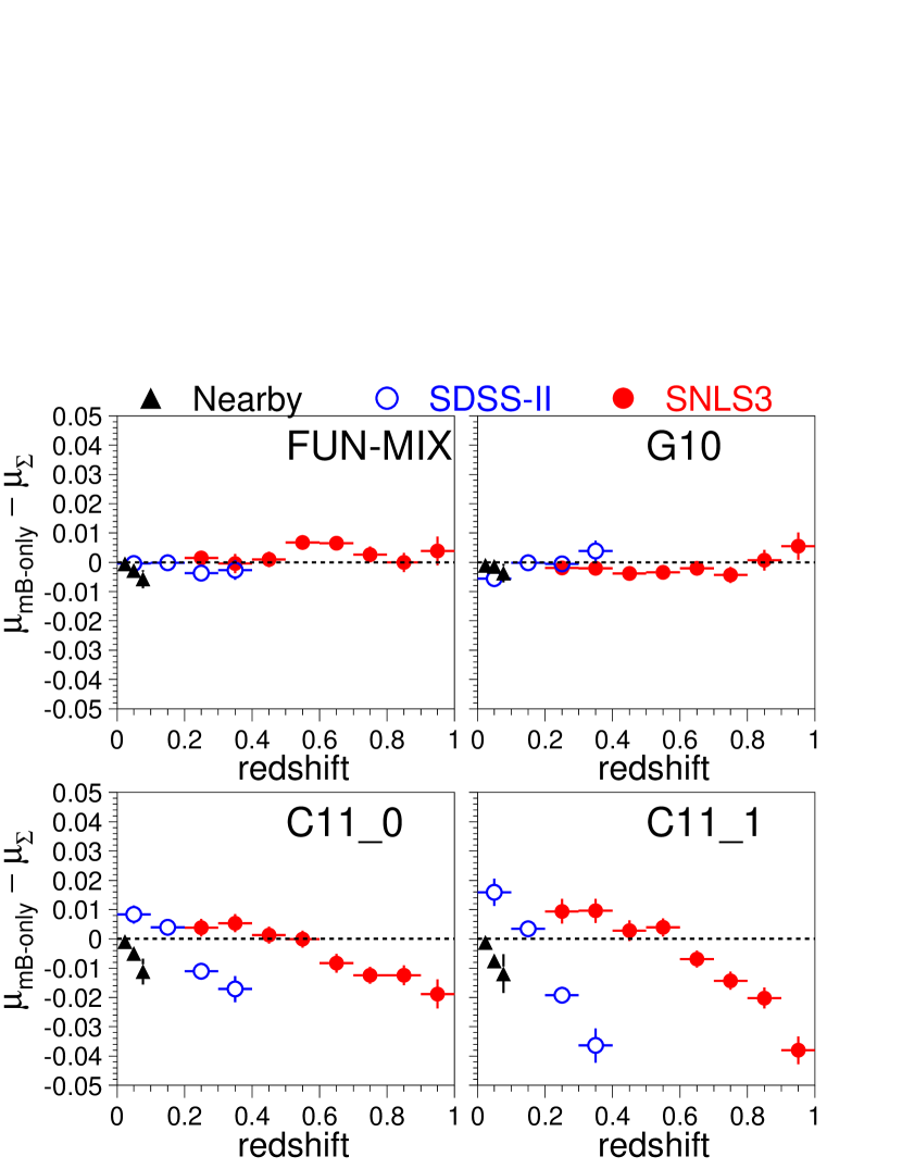
Figure 12.— Average difference between the distance modulus from the $m_{B}$-only fit and that from the $\Sigma$-fit, vs. redshift. The simulated (true) scatter model is indicated in each panel. The simulated samples are nearby (solid triangles), SDSS–II (open circles), and SNLS3 (solid circles).

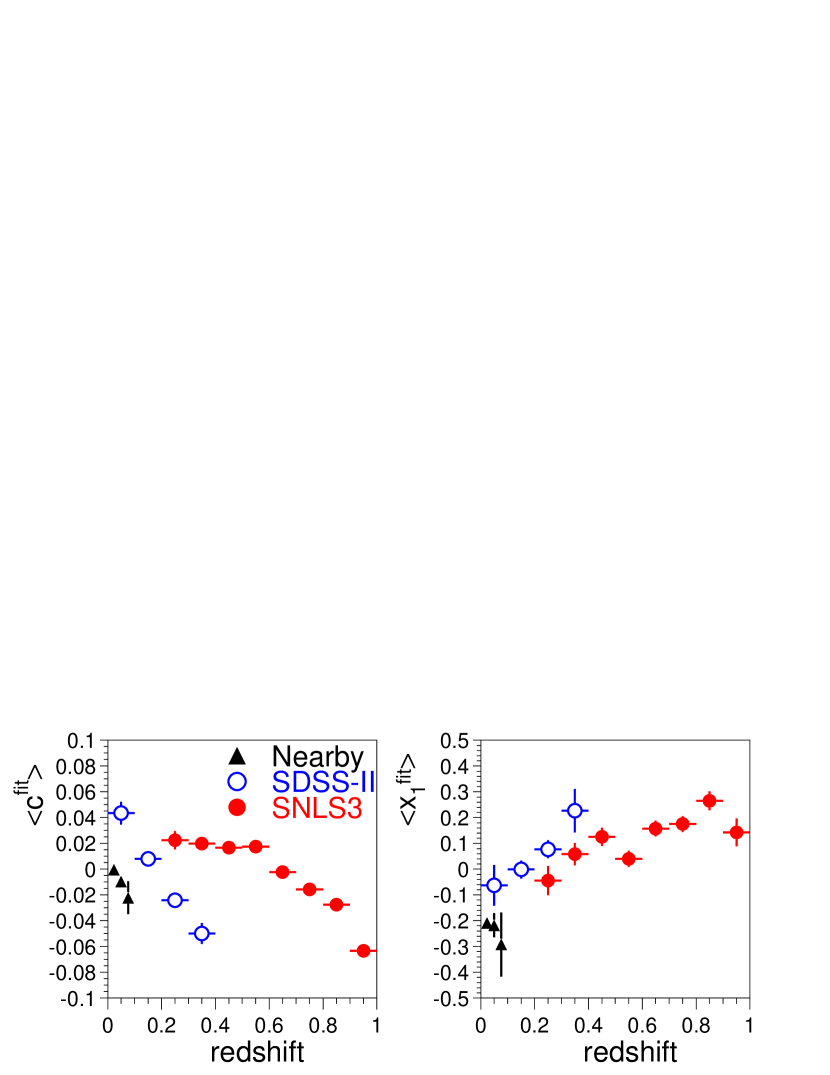
Figure 13.— Mean fitted salt-ii color vs. redshift for the nearby (solid triangles), SDSS–II (open blue circles) and SNLS3 (solid red circles) simulation. Right panel shows mean fitted salt-ii stretch parameters ($x_{1}$) vs. redshift. Although this simulation uses the G10 intrinsic scatter model, there is little difference for the other scatter models. Also note that the analogous plots in the bottom panels of Figures 1 and 2 show a larger variation because of the more strict selection requirement of three passbands with S/N$>8$.

6.3. Estimating the $w$-bias

To estimate the bias on the dark energy parameter $w$, we fit the simulated Hubble diagram in a manner similar to that described in Section 8 of K09. The effect of Malmquist corrections is discussed later in Section 6.4. The $w$-bias is defined to be the difference between $w$ obtained from the $m_{B}$-only method and the $\Sigma$-fit method. Priors are included from measurements of baryon acoustic oscillations from the SDSS Luminous Red Galaxy sample (Eisenstein et al., 2005) and from the cosmic microwave background temperature anisotropy measured from the Wilkinson Microwave Anistropy Probe (Komatsu et al., 2009).

Since the simulated SN sample consists of $20$ times the data statistics, the uncertainties on the priors have been reduced by a factor of $\sqrt{20}$. We checked this procedure by splitting the simulated sample into $20$ independent sub-samples and fitting each sub-sample with the nominal priors; the average of the $20$ fitted $w$-values is in good agreement with that from using the full simulation and priors with reduced uncertainties. The $\beta$-bias and Malmquist-uncorrected $w$-bias values are defined as the difference between the $m_{B}$-only and $\Sigma$-fit methods, and they are shown in Table 6.2. The uncertainty on the $w$-bias is given by ${\rm rms}/\sqrt{20}$, where rms is the dispersion among the $20$ independent $w$-bias measurements.

For the FUN-MIX and G10 models the $w$-bias is small ($<0.02$) for all sample combinations. This small bias is expected since the fitted $\beta$ and distance moduli show a very small bias. For the C11 models, the $w$-bias is larger. Fitting the SDSS–II or SNLS3 sample alone, the $w$-bias is $\sim 0.07$ for the C11_0 model and $\sim 0.12$ for the C11_1 model. Combining the SDSS–II $+$ SNLS3 samples, the $w$-bias is reduced by a factor of $\sim 2$ for each of the C11 models. Including the nearby sample (nearby+SDSS–II+SNLS3) the $w$-bias is further reduced: $0.01$ and $0.02$ for the C11_0 and C11_1 models, respectively. The reduction in $w$-bias as more samples are combined is a result of the fortuitous circumstance that the mean salt-ii color for each sample is very close: $-0.005$, $-0.015$, and $-0.005$ for the nearby, SDSS–II, and SNLS3, respectively. To illustrate this point we have redone the analysis using a simulated nearby sample that has no Malmquist bias and a mean salt-ii color that is 0.06 mag redder than the data; the resulting $w$-bias on the combined nearby+SDSS–II+SNLS3 sample increases to 0.05.

6.4. Monte Carlo Correction for Malmquist Bias

In Section 6.3 the $w$-bias is determined without accounting for differences in the Malmquist bias correction. While the true Malmquist bias should not depend on the analysis method ($m_{B}$-only versus $\Sigma$-method), here we show that the evaluated Malmquist bias, using the fitted value of $\beta$, does indeed depend on the analysis method. In addition, using the evaluated Malmquist bias reduces the $\mu$-bias shown in Figure 12. In the discussion below, “MqSIM” refers to the simulation used to evaluate the Malmquist bias correction.

For the $\Sigma$-fit method the MqSIM uses the correct model of intrinsic scatter and the correct $\alpha$ and $\beta$ parameters. In principle the intrinsic-scatter matrix would have to be translated into a wavelength-dependent scatter model for the simulation, but we have not preformed this step. For the $m_{B}$-only method the MqSIM for each sample uses the G10 model and the fitted (biased) value of $\beta_{\rm fit}$ from Table 6.2. This procedure is used because it closely reflects the procedure in previous analyses. The distance-modulus corrections are from a second-order polynomial fit to $\mu_{\rm fit}-\mu_{\rm true}$ versus redshift: $\mu_{\rm true}$ is the true distance modulus in the MqSIM, and $\mu_{\rm fit}$ is the distance computed from the SALT2-fitted parameters (color and stretch) and the simulated values of $\alpha$ and $\beta$.

Figure 14 shows the $\mu$-bias versus redshift with the Malmquist correction applied. Overall the redshift-dependent bias is smaller than for the uncorrected distances in Figure 12, but the bias is still significant for the C11 models. The bias is zero for the G10 model because the fitted light curve model (G10) corresponds to the correct model of intrinsic scatter. The Malmquist-corrected $w$-bias results are shown in the last column of Table 6.2. Compared to the bias from the uncorrected Hubble diagrams, the $w$-bias is typically smaller when the Malmquist correction is applied.

While using an incorrect model of intrinsic scatter can lead to a significant bias in the Hubble diagram, this bias is somewhat reduced by simply applying a simulated Malmquist bias correction using the fitted value of $\beta$ in the simulation. The bias reduction depends on the intrinsic scatter model, and we cannot rule out increased sensitivity on other systematic effects.

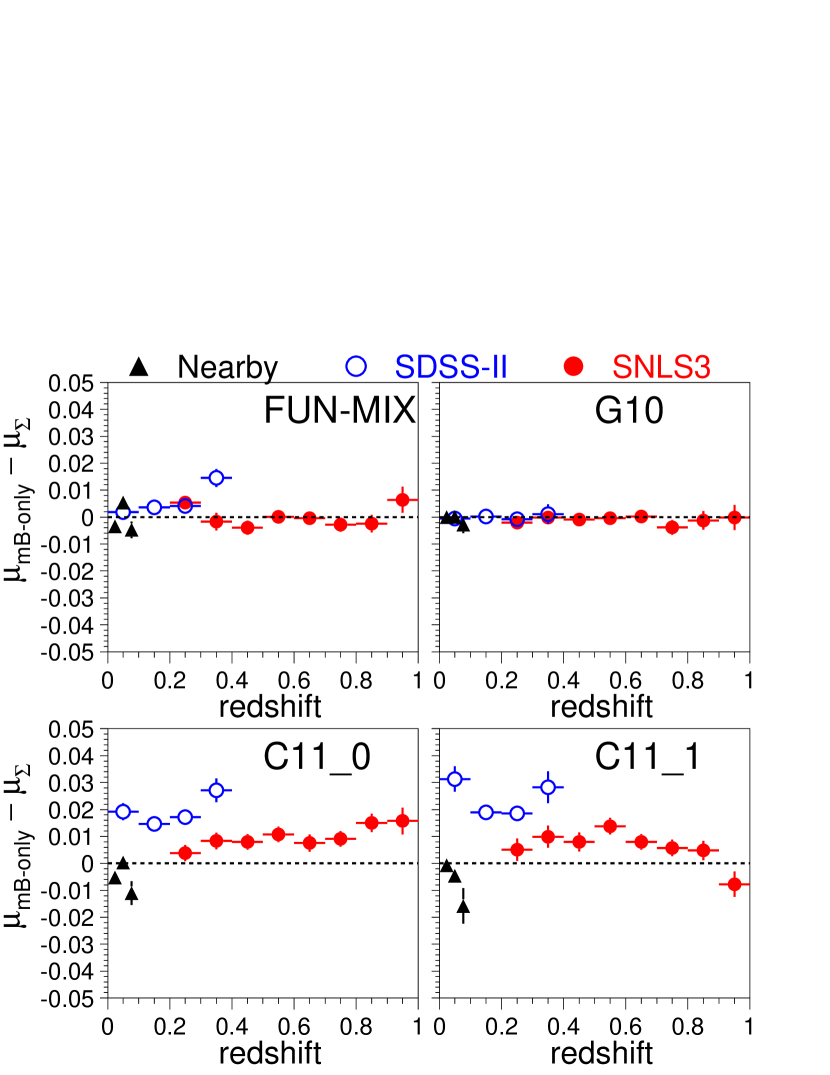
Figure 14.— Same as Figure 12, but after applying Malmquist bias correction.

7. Conclusions

We have used high quality SDSS–II and SNLS3 data and simulations to show that SN Ia intrinsic brightness variations include wavelength dependent variations resulting in a color dispersion of $\sim 0.02$ mag. A broad range of simulated intrinsic-scatter models (Table 3) is roughly consistent with the following photometric observables: Hubble scatter, dispersion in $B-V-c^{\prime}$, and photo-$z$ residuals. These models include the G10 model that is dominated by a coherent term and has only positive wavelength correlations, and the C11 model that has a small coherent term and large anti-correlations.

We have used these intrinsic scatter models in high-statistics simulations to test the standard procedure of adding a constant distance-modulus uncertainty ($\sigma_{\rm int}$) to the measured uncertainties so that $\chi^{2}/N_{\rm dof}=1$ for cosmology fits to the SN Ia Hubble-diagram. The constant $\sigma_{\rm int}$ assumption is valid if the light curve fits include model uncertainties with the correct wavelength dependence of the scatter. If these model uncertainties are not correct, such as using the salt-ii uncertainties to fit a simulated sample with large anti-correlations in the scatter (C11 model), then significant biases can appear in the Hubble diagram. For the specific simulation tests reported here the distance-modulus bias varies by up to 0.05 mag over the redshift range of the each survey, although this bias is roughly halved after applying Malmquist bias corrections. For the combined nearby+SDSS–II+SNLS3 simulated sample, which corresponds closely to the 472 SNe Ia analyzed in Sullivan et al. (2011), the $w$-bias is only $\sim 0.02$, in part because the mean color for each sample is very nearly the same. While this $w$-bias is well below the total systematic uncertainty reported in Sullivan et al. (2011) ($\delta w_{\rm syst}=0.06$), there is no assurance that future analyses on larger data sets will benefit from the fortuitous cancellations. For example, replacing the biased nearby sample with an unbiased sample increases the $w$-bias to $0.05$, comparable to the current systematic uncertainty.

We have also shown that applying a simulated Malmquist bias correction, based on the fitted (biased) $\beta$ value, may reduce the bias from using an incorrect model of intrinsic scatter. However, we urge caution in relying on this apparent “free lunch” because we have not fully explored if this naive correction increases the sensitivity to other systematic effects.

It is important not to interpret our results as proof that such biases exist in current SNIa-cosmology results; we have shown, for example, that this intrinsic scatter bias is negligible if the G10 model is correct. However, until the intrinsic scatter correlations can be better constrained, our results suggest that an additional systematic uncertainty should be included.

Although the intrinsic-scatter models considered here depend only on wavelength (except for the KRW09 models), the true behavior could include a dependence on epoch, color, stretch, and redshift. The impact of the scatter models on the salt-ii training is under investigation and will be published later. To obtain more robust systematic constraints on cosmological parameters, we encourage additional studies to measure or constrain the nature of intrinsic scatter.

J.F. and R.K. are grateful for the support of National Science Foundation grant 1009457, a grant from “France and Chicago Collaborating in the Sciences” (FACCTS), and support from the Kavli Institute for Cosmological Physics at the University of Chicago.

The SDSS is managed by the Astrophysical Research Consortium for the Participating Institutions. The Participating Institutions are the American Museum of Natural History, Astrophysical Institute Potsdam, University of Basel, Cambridge University, Case Western Reserve University, University of Chicago, Drexel University, Fermilab, the Institute for Advanced Study, the Japan Participation Group, Johns Hopkins University, the Joint Institute for Nuclear Astrophysics, the Kavli Institute for Particle Astrophysics and Cosmology, the Korean Scientist Group, the Chinese Academy of Sciences (LAMOST), Los Alamos National Laboratory, the Max-Planck-Institute for Astronomy (MPA), the Max-Planck-Institute for Astrophysics (MPiA), New Mexico State University, Ohio State University, University of Pittsburgh, University of Portsmouth, Princeton University, the United States Naval Observatory, and the University of Washington.

This work is based in part on observations made at the following telescopes. The Hobby-Eberly Telescope (HET) is a joint project of the University of Texas at Austin, the Pennsylvania State University, Stanford University, Ludwig-Maximillians-Universität München, and Georg-August-Universität Göttingen. The HET is named in honor of its principal benefactors, William P. Hobby and Robert E. Eberly. The Marcario Low-Resolution Spectrograph is named for Mike Marcario of High Lonesome Optics, who fabricated several optical elements for the instrument but died before its completion; it is a joint project of the Hobby-Eberly Telescope partnership and the Instituto de Astronomía de la Universidad Nacional Autónoma de México. The Apache Point Observatory 3.5 m telescope is owned and operated by the Astrophysical Research Consortium. We thank the observatory director, Suzanne Hawley, and site manager, Bruce Gillespie, for their support of this project. The Subaru Telescope is operated by the National Astronomical Observatory of Japan. The William Herschel Telescope is operated by the Isaac Newton Group on the island of La Palma in the Spanish Observatorio del Roque de los Muchachos of the Instituto de Astrofisica de Canarias. The W.M. Keck Observatory is operated as a scientific partnership among the California Institute of Technology, the University of California, and the National Aeronautics and Space Administration. The Observatory was made possible by the generous financial support of the W. M. Keck Foundation.

Appendix A Simulation of Nearby SN Ia Sample

Here we describe the simulation of the nearby ($z<0.1$) SN Ia sample corresponding to the 123 nearby SNe Ia used in Conley et al. (2011). While the nearby SN data are from several surveys and filter sets, we simplify the simulation by considering only the CFA3-Keplercam light curves (Hicken et al., 2009) using the $UBVr$ filters. The $i$ band is dropped because it is outside the valid wavelength range of the salt-ii model. Since the CFA3-Keplercam simulation is a proxy for the entire nearby SN sample, we simulate the correct nearby-SN statistics corresponding to about half that of the SNLS3 sample.

Since we do not have the observing conditions (mainly PSF and sky noise) needed for the SNANA simulation, we adopt a different strategy. The basic idea is to use each observed SN to define an observational sequence. The observed redshift and time of peak brightness are used along with the cadence. A random salt-ii stretch and color are chosen for each SN, and the simulated S/N for each epoch is essentially scaled from the observed S/N. More technically, we artificially fixed the PSF to be $0.8^{\prime\prime}$ and then for each epoch compute the sky noise needed to simulate the observed uncertainty; this strategy allows generating nearby SNe in exactly the same manner as for the SDSS–II and SNLS3. With little knowledge of the spectroscopic selection criteria we cannot simulate the selection bias from first principles. We therefore modified the population parameters in Table 1 so that the simulated color and stretch distributions match those of the nearby sample. For the generated color distribution the peak-probability value depends on redshift, $-0.02-z/2$, and the Gaussian width parameters are $\sigma_{-}=0.06$ and $\sigma_{+}=0.10$. For the generated stretch distribution, the peak-probability value is reduced to 0.2.

The intrinsic-scatter matrix is determined for the nearby sample with the same procedure used on the SDSS–II and SNLS3 simulations, and using SALT2mu we have checked that the fitted $\beta$ values are in good agreement with the simulated input, $\beta_{\rm SIM}=3.2$. We have also examined the analogous data/MC comparisons in Figures 1 and 2, and find equally good agreement.

References

- Aldering et al. (2002) Aldering, G. et al. 2002, in Society of Photo-Optical Instrumentation Engineers (SPIE) Conference Series, Vol. 4836, Society of Photo-Optical Instrumentation Engineers (SPIE) Conference Series, ed. J. A. Tyson & S. Wolff, 61–72
- Astier et al. (2006) Astier, P. et al. 2006, A&A, 447, 31
- Bailey et al. (2009) Bailey, S. et al. 2009, A&A, 500, L17
- Blondin et al. (2011) Blondin, S., Mandel, K. S., & Kirshner, R. P. 2011, A&A, 526, A81
- Blondin et al. (2011) Blondin, S. et al. 2011, MNRAS, 417, 1280
- Chotard (2011) Chotard, N. 2011, PhD thesis, University Claude Bernard Lyon, 1, Lyon, France
- Chotard et al. (2011) Chotard, N. et al. 2011, A&A, 529, L4
- Conley et al. (2011) Conley, A. et al. 2011, ApJS, 192, 1
- Dilday et al. (2008) Dilday, B. et al. 2008, ApJ, 682, 262
- Eisenstein et al. (2005) Eisenstein, D. et al. 2005, ApJ, 633, 560
- Freedman et al. (2009) Freedman, W. et al. 2009, ApJ, 704, 1036
- Frieman et al. (2008) Frieman, J. A. et al. 2008, AJ, 135, 338
- Fukugita et al. (1996) Fukugita, M. et al. 1996, AJ, 111, 1748
- Gunn et al. (1998) Gunn, J. E. et al. 1998, AJ, 116, 3040
- Gunn et al. (2006) —. 2006, AJ, 131, 2332
- Guy et al. (2010) Guy, J. et al. 2010, A&A, 523, A7
- Hicken et al. (2009) Hicken, M. et al. 2009, ApJ, 700, 331
- Holtzman et al. (2008) Holtzman, J. et al. 2008, AJ, 136, 2306
- Kasen et al. (2009) Kasen, D., Röpke, F. K., & Woosley, S. E. 2009, Nature, 460, 869
- Kasen et al. (2006) Kasen, D., Thomas, R. C., & Nugent, P. 2006, ApJ, 651, 366
- Kessler et al. (2009a) Kessler, R. et al. 2009a, ApJS, 185, 32
- Kessler et al. (2009b) —. 2009b, PASP, 121, 1028
- Kessler et al. (2010) Kessler, R. et al. 2010, ApJ, 717, 40
- Komatsu et al. (2009) Komatsu, E. et al. 2009, ApJS, 180, 330
- Lampeitl et al. (2010) Lampeitl, H. et al. 2010, ApJ, 722, 566
- Lupton et al. (2001) Lupton, R. et al. 2001, in ASP Conf. Ser. 238: Astronomical Data Analysis Software and Systems X, ed. F. R. Harnden, Jr., F. A. Primini, & H. E. Payne, 269–+
- Mandel et al. (2011) Mandel, K. S., Narayan, G., & Kirshner, R. P. 2011, ApJ, 731, 120
- March et al. (2011) March, M. C. et al. 2011, MNRAS, 418, 2308
- Marriner et al. (2011) Marriner, J. et al. 2011, ApJ, 740, 72
- Perlmutter et al. (1999) Perlmutter, S. et al. 1999, ApJ, 517, 565
- Perrett et al. (2010) Perrett, K. et al. 2010, AJ, 140, 518
- Phillips (1993) Phillips, M. M. 1993, ApJ, 413, 105
- Riess et al. (1998) Riess, A. et al. 1998, AJ, 116, 1009
- Riess et al. (1996) Riess, A. G., Press, W. H., & Kirshner, R. P. 1996, ApJ, 473, 88
- Riess et al. (2004) Riess, A. G. et al. 2004, ApJ, 607, 665
- Sako et al. (2008) Sako, M. et al. 2008, AJ, 135, 348
- Schlegel et al. (1998) Schlegel, D. J., Finkbeiner, D. P., & Davis, M. 1998, ApJ, 500, 525
- Silverman et al. (2012) Silverman, J. M. et al. 2012, MNRAS, 425, 1889
- Smith et al. (2012) Smith, M. et al. 2012, ApJ, 755, 61
- Sullivan et al. (2006) Sullivan, M. et al. 2006, ApJ, 648, 868
- Sullivan et al. (2011) Sullivan, M. et al. 2011, ApJ, 737, 102
- Tripp (1997) Tripp, R. 1997, A&A, 325, 871
- Wood-Vasey et al. (2007) Wood-Vasey, W. M. et al. 2007, ApJ, 666, 694
- York et al. (2000) York, D. G. et al. 2000, AJ, 120, 1579
- Zheng et al. (2008) Zheng, C. et al. 2008, AJ, 135, 1766