Why do the braking indices of pulsars span a range of more than 100 millions?

Abstract

Here we report that the observed braking indices of the 366 pulsars in the sample of Hobbs et al. range from about $-10^{8}$ to about $+10^{8}$ and are significantly correlated with their characteristic ages. Using the model of magnetic field evolution we developed previously based on the same data, we derived an analytical expression for the braking index, which agrees with all the observed statistical properties of the braking indices of the pulsars in the sample of Hobbs et al. Our model is, however, incompatible with the previous interpretation that magnetic field growth is responsible for the small values of braking indices ($<3$) observed for “baby” pulsars with characteristic ages of less than $2\times 10^{3}$ yr. We find that the “instantaneous” braking index of a pulsar may be different from the “averaged” braking index obtained from fitting the data over a certain time span. The close match between our model-predicted “instantaneous” braking indices and the observed “averaged” braking indices suggests that the time spans used previously are usually smaller than or comparable to their magnetic field oscillation periods. Our model can be tested with the existing data, by calculating the braking index as a function of the time span for each pulsar. In doing so, one can obtain for each pulsar all the parameters in our magnetic field evolution model, and may be able to improve the sensitivity of using pulsars to detect gravitational waves.

1. Introduction

Assuming the braking law of a pulsar as

$$\dot{\nu}=-K\nu^{n_{\rm b}},$$ (1)

where $\nu$ is its spin frequency and $n_{\rm b}$ is called its braking index, Manchester & Taylor (1977) found that

$$n_{\rm b}=\ddot{\nu}\nu/\dot{\nu}^{2},$$ (2)

if $\dot{K}=0$. For the standard magnetic dipole radiation model with constant magnetic field ($\dot{K}=0$), $n_{\rm b}=3$. Therefore $n_{\rm b}\neq 3$ indicates some deviation from the standard magnetic dipole radiation model with constant magnetic field.

Blandford & Romani (1988) re-formulated the braking law of a pulsar as,

$$\dot{\nu}=-K(t)\nu^{3}.$$ (3)

This means that the standard magnetic dipole radiation is responsible for the instantaneous spin-down of a pulsar, but the braking torque determined by $K(t)$ may be variable. In this formulation, $n_{\rm b}\neq 3$ does not indicate deviation from the standard magnetic dipole radiation model, but means only that $K(t)$ is time dependent. From Equation (3) one can obtain,

$$\frac{\dot{K}}{K}\frac{\nu}{\dot{\nu}}={n_{\rm b}}-3.$$ (4)

Assuming that magnetic field evolution is responsible for the variation of $K(t)$, we have $K=AB(t)^{2}$, in which $A$ is a constant and $B(t)$ is the time variable dipole magnetic field strength of a pulsar. The above equation then suggests that $n_{\rm b}<3$ indicates magnetic field growth of a pulsar, and vice versa, since $\dot{\nu}<0$ and $K>0$. This can be seen more clearly from (Zhang & Xie 2012b; hereafter Paper I),

$$\dot{K}=\frac{\ddot{\nu}}{\nu^{3}}(\frac{3}{n_{\rm b}}-1)=\frac{\dot{\nu}^{2}}{\nu^{4}}(3-n_{\rm b}).$$ (5)

Many authors have thus used the observed $n_{\rm b}<3$ of some very young pulsars to infer their possible magnetic field increase (e.g., Blandford & Romani 1988; Chanmugam & Sang 1989; Manchester & Peterson 1989; Lyne et al. 1993, 1996; Johnston & Galloway 1999; Wu et al. 2003; Lyne 2004; Chen & Li 2006; Livingstone et al. 2006, 2007; Middleditch et al. 2006; Yue et al. 2007; Espinoza et al. 2011). Magnetospheric activities or fall-back accretion may also be able to produce $n_{\rm b}<3$ (e.g. Menou et al. 2001; Alpar et al. 2001; Xu & Qiao 2001; Wu et al. 2003; Chen & Li 2006; Yue et al. 2007). This can also be explained by another model based on a decrease in effective moment of inertia due to an increase in the fraction of the stellar core that becomes superfluid as the star cools via neutrino emission (Ho & Andersson 2012).

However, the above studies have not investigated the statistical properties of the braking indices of pulsars. Recently, Magalhaes et al. (2012) studied the observed braking indices of several very young pulsars statistically. They built a model of a pulsar’s braking law to explain the ranges of these observed braking indices, and then predicted the possible values of the braking indices of several other very young pulsars withusing only their measured $\nu$ and $\dot{\nu}$. Testing these predictions and applying the model to more pulsars for observational tests may shed light on our further understanding of pulsars.

In Paper I, we have shown that the observed $n_{\rm b}$, for the large sample of pulsars reported by Hobbs et al. (2010, hereafter H2010), not only deviates from $n_{\rm b}=3$, but also ranges from around $-10^{8}$ to around $+10^{8}$, i.e., spanning a range of more than 100 millions, which has not been explained so far. In this work, we will first apply the model of Magalhaes et al. (2012) to this sample, and then search for possible correlations of the observed $n_{\rm b}$ of pulsars in the sample of H2010. We find a significant correlation between $n_{\rm b}$ and the characteristic ages of pulsars, which is explained satisfactorily with the magnetic field evolution model we developed in Paper I. Finally we will make a testable prediction of our model and discuss its physical implications.

2. Applicability of the model of Magalhaes et al. (2012) to the pulsars in H2010

Magalhaes et al. (2012) used equation (1) to predict,

$$n_{\rm pre}=\frac{\log(|\dot{\Omega}|S^{2}/\xi^{2})}{\log(\Omega)},$$ (6)

where $\Omega=2\pi\nu$, $S=2.3\times 10^{20}$ Hz^1/2 G and is assumed to be the same for all pulsars, and $1.5\times 10^{13}<\xi<34\times 10^{13}$ in units of Hz${}^{(3-n_{\rm b})/2}$ G determines the range of $n_{\rm pre}$ for each pulsar. Magalhaes et al. (2012) showed that Equation (6) describes the ranges of $n_{\rm b}$ observed for several very young pulsars very well. A natural question arises: can this model also explain the observed $n_{\rm b}$ for other older pulsars of the sample of H2010? In Figure 1 we plot the distributions of the observed braking indices ($n_{\rm obs}=\ddot{\nu}\nu/\dot{\nu}^{2}$) of the pulsars of the sample of H2010 and the ratios between $n_{\rm obs}$ and $n_{\rm pre}$. $n_{\rm obs}$ spans a range from around $-10^{8}$ to around $+10^{8}$, as shown in Paper I. However, $n_{\rm obs}/n_{\rm pre}$ spans a similar range and has almost the same numbers of positive and negative values. This means that the model of Magalhaes et al. (2012) cannot explain both the magnitudes and signs of the braking indices of the pulsars of the sample of H2010. Therefore an alternative model is needed to account for the observed braking indices of these pulsars.

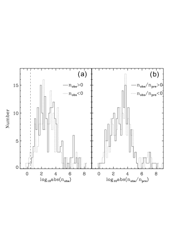
Figure 1.— (a) Distributions of the observed braking indices ($n_{\rm obs}=\ddot{\nu}\nu/\dot{\nu}^{2}$). (b) Ratios of the observed and predicted braking indices ($n_{\rm pre}$) from Equation (6) (equation  (11) in Magalhaes et al. 2012).

3. Observed correlations of braking indices

In order to develop a model to account for the observed braking indices of the pulsars of the sample of H2010, we first explore possible correlations of the observed braking index $n_{\rm b}=\ddot{\nu}\nu/\dot{\nu}^{2}$ with various spin-down parameters and their combinations, as shown in Figure 2. No or only weak correlation is found either between $n_{\rm b}$ and $\nu$ or between $n_{\rm b}$ and $\ddot{\nu}$. Strong correlations are found both between $n_{\rm b}$ and $\dot{\nu}$ and between $n_{\rm b}$ and the characteristic age $\tau_{\rm c}=-\frac{\nu}{2\dot{\nu}}$; the latter correlation is very significant and is the focus of study in the rest of this work.

The $n_{\rm b}\sim\tau_{\rm c}$ correlation shown in the bottom panel of Figure 2 reveals three phenomena. (1) For all young pulsars with $10^{4}<\tau_{\rm c}<5\times 10^{4}$ yr, $10<n_{\rm b}<40$ and $n_{\rm b}$ is not correlated with $\tau_{\rm c}$. (2) Excluding these pulsars, the overall correlation is almost linear over about eight orders of magnitude for both $n_{\rm b}$ and $\tau_{\rm c}$. (3) The overall correlation is almost the same for positive or negative $n_{\rm b}$.

Figure 2.— Observed correlations of the braking index $n_{\rm b}$ with (from top to bottom) $\nu$, $\dot{\nu}$, $\ddot{\nu}$ and $\tau_{\rm c}$.

4. A new analytical model of braking index

In Paper I, we have shown that the observed correlations between $\ddot{\nu}$ and other observables or parameters can be well explained by assuming that the braking law takes the form of Equation (3) and the evolution of the dipole magnetic field of a pulsar consists of a long-term decay modulated by one or multiple oscillation components, i.e.,

$$B(t)=B_{0}(\frac{t}{t_{0}})^{-\alpha}(1+k\sin(\phi+2\pi\frac{t}{T})),$$ (7)

where $t_{0}$ and $B_{0}$ are the initial decay time and dipole magnetic field strength, $\alpha$ is the decay index, and $k$, $\phi$ and $T$ are the oscillation amplitude, initial oscillation phase, and oscillation period, respectively. In Paper I we have shown that $\alpha\geq 0.5$, but its upper limit cannot be well constrained with the existing data. In this work, we simply take $\alpha=0.5$ for simplicity; the conclusions of this work will not change for larger values of $\alpha$.

From Equation (3), we can solve for the spin evolution of a pulsar,

$$\nu^{-2}=\nu_{0}^{-2}+2\int_{t_{0}}^{t}K(t)dt.$$ (8)

With $K=AB(t)^{2}$ and Equation (7), we have

$$\tau_{\rm c}=-\frac{\nu}{2\dot{\nu}}=\frac{1}{2K\nu^{2}}\approx t\ln\frac{t}{t_{0}},$$ (9)

where $\alpha=0.5$ and $k\ll 1$ are assumed. It is noticeable that the oscillation term in Equation (7) is not important in the above relation, since $k\ll 1$. However the decay component of Equation (7) makes the real age of a pulsar significantly shorter than its characteristics age, since normally $t/t_{0}\gg 1$ (Zhang & Xie, 2012a).

From Equation (8) we can easily obtain $\dot{\nu}(t)$ and $\ddot{\nu}(t)$. Inserting $\nu(t)$, $\dot{\nu}(t)$ and $\ddot{\nu}(t)$ into Equation (2), we have,

$$n_{\rm b}=3+\ln\frac{t}{t_{0}}(2-4ftC(t))=3+\frac{\tau_{\rm c}}{t}(2-4ftC(t)),$$ (10)

where $f=\frac{2\pi k}{T}$ and $C(t)=\cos(\phi+2\pi\frac{t}{T})$. As we have shown in Paper I, the oscillatory term can be ignored in determining $\ddot{\nu}$, so young pulsars with $\tau_{\rm c}\leq 10^{5}$ have $\ddot{\nu}>0$. Ignoring the oscillatory term in Equation (10), we have

$$n_{\rm b}\approx 3+2\frac{\tau_{\rm c}}{t}=3+2\ln\frac{t}{t_{0}},$$ (11)

which for young pulsars gives $n_{\rm b}>0$ (since $t>t_{0}$) and $n_{\rm b}$ is not well correlated with $\tau_{\rm c}$, in agreement with the data shown in the lower left corner of the bottom panel in Figure 2. For old pulsars, the oscillatory term dominates and thus Equation (10) gives,

$$n_{\rm b}\approx\pm 4\tau_{\rm c}f,$$ (12)

since $C(t)$ most likely takes values around $+1$ or $-1$. This immediately suggests that $n_{\rm b}$ should be linearly correlated with $\tau_{\rm c}$ and have equal probabilities to be either positive or negative, again in agreement with the correlation shown in the bottom panel of Figure 2.

In Figure 3, we plot the analytically calculated $n_{\rm b}$ as a function of $\tau_{\rm c}$ using Equations (9) and (10) for $k=10^{-4}$ and $10^{-5}$, respectively; we also assume $t_{0}=0.5$ yr and $T=10$ yr, the latter is the typical time scale of the quasi-periodic features in the power spectra of the timing residuals reported in H2010. The upper boundary in each panel is obtained when $C(t)=\pm 1$ and the other values of $n_{\rm b}$ are obtained when $-1<C(t)<1$. Clearly the observed correlation shown in Figure 2 is well reproduced. In particular, the lack of $n_{\rm b}<0$ for young pulsars with $\tau_{\rm c}$ is predicted with $k\leq 10^{-4}$, which in our model is caused by their long term magnetic field decay.

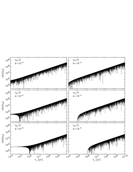
Figure 3.— Analytically calculated $n_{\rm b}$ as a function of $\tau_{\rm c}$ using Equation (10), for different values of $k$.

Equation (10) can be rewritten as,

$$n_{\rm b}/\tau_{\rm c}=3/\tau_{\rm c}+2/t-4fC(t)\approx 3/\tau_{\rm c}+2/t\pm 4f.$$ (13)

In Figure 4, we show the observed correlation between $n_{\rm b}/\tau_{\rm c}$ and $\tau_{\rm c}$, overplotted with the analytical results of Equation (13) with $T=10$ yr and $k=10^{-3},\ 10^{-4}$ and $10^{-5}$, respectively. Once again, the analytical results agree quite well with the data quite well.

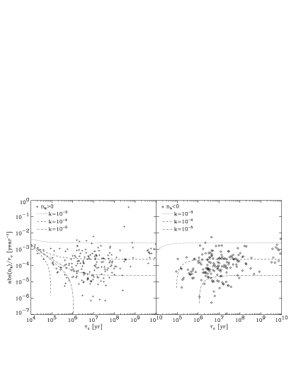
Figure 4.— Correlation between $n_{\rm b}/\tau_{\rm c}$ and $\tau_{\rm c}$. The different curves show the analytically calculated model predictions using Equation (13) for different values of $k$.

5. On “baby” pulsars and young pulsars

As discussed above, $n_{\rm b}<3$ has been well established for all very young pulsars with $\tau_{\rm c}<2\times 10^{3}$ yr (Livingstone et al. 2007), which we call “baby” pulsars here for convenience. In Figure 5 we show a comparison between all the measured braking indices of “baby” pulsars and those of young pulsars with $10^{4}<\tau_{\rm c}<10^{5}$ yr. From Equation (5), we get $\dot{K}>0$ or $\dot{K}<0$ for “baby” pulsars or young pulsars, respectively. If $\dot{K}\neq 0$ is due to $\dot{B}\neq 0$, we are then led to the scenario that the magnetic fields of “baby” pulsars grow, but those of young pulsars decay. If these “baby” pulsars with $\tau_{\rm c}<2\times 10^{3}$ yr evolve to become young pulsars, this must happen when the time of transition from the growth phase to the decay phase is longer than the ages of these “baby” pulsars, i.e., $t_{0}^{\rm baby}\geq 10^{3}$ yr. For a typical young pulsar with $\tau_{\rm c}\sim 2\times 10^{4}$ yr and $n_{\rm b}\sim 20$, Equation (11) gives $t\sim 2.4\times 10^{3}$ and $t_{0}^{\rm young}\sim 0.5$ yr. The mismatch between $t_{0}^{\rm baby}$ and $t_{0}^{\rm young}$ suggests that significantly different mechanisms are responsible for the observed braking indices for “baby” and young pulsars, respectively. In other words, our model that $n_{\rm b}\neq 3$ is due to $\dot{B}\neq 0$ can only be applied to young (and old pulsars), but not to “baby” pulsars. Indeed, we may expect significant fall-back accretion or neutrino cooling only for “baby” pulsars; these mechanisms have previously also been suggested to be responsible for the observed $n_{\rm b}<3$ of these “baby” pulsars. In either case, the additional torque of accretion or the reduced moment of inertia due to an increased fraction of superfluid stellar core can result in $n_{\rm b}<3$. Stronger magnetospheric activities are also expected from “baby” pulsars, whose magnetic fields should be stronger than those of young pulsars.

Figure 5.— Comparison between the measured braking indices of “baby” pulsars (in the lower left corner; data from Livingstone et al. 2007) and those of young pulsars (in the upper right corner; data from H2010).

6. Model prediction: the effect of time span

All the above equations for $n_{\rm b}$ give $n_{\rm b}$ as a function of $t$, i.e., the calculated $n_{\rm b}$ is in fact a function of time for a given pulsar, as shown in the left panel of Figure 6, in which the horizontal axis “Time” is the calendar time. We call $n_{\rm b}$ calculated this way the “instantaneous” braking index. However, in analyzing the observed timing data of a pulsar, one usually fits the data on time of arrival (TOA) over a certain time span to a Taylor expansion to third order:

$$\Phi(t)=\Phi_{0}+\nu_{0}(t-t_{0})+\frac{1}{2}\dot{\nu}_{0}(t-t_{0})^{2}+\frac{1}{6}\ddot{\nu}_{0}(t-t_{0})^{3},$$ (14)

where $\Phi(t)$ is the phase of TOA of the observed pulses, and $\Phi_{0}$, $\nu_{0}$, $\dot{\nu}_{0}$ and $\ddot{\nu}_{0}$ are the values of these parameters at $t_{0}$, to be determined from the fitting. $n_{\rm b}$ calculated from $\nu_{0}$, $\dot{\nu}_{0}$ and $\ddot{\nu}_{0}$ is thus not exactly the same as the “instantaneous” braking index. We call $n_{\rm b}$ calculated this way over a certain time span the “averaged” braking index.

In the right panel of Figure 6, we show the simulated result for the “averaged” braking index as a function of time span, In this simulation, we first produce a series of TOAs using Equations (8) and (7), and then use Equation (14) to obtain $\nu_{0}$, $\dot{\nu}_{0}$ and $\ddot{\nu}_{0}$ for different lengths of time span. It can be seen that the “averaged” $n_{\rm b}$ is close to the “instantaneous” one when the time span is shorter than $T$, which is the oscillation period of the magnetic field. The close match between our model predicted “instantaneous” $n_{\rm b}$ and the observed “averaged” $n_{\rm b}$, as shown in Figure 4 suggests that the time spans used in the H2010 sample are usually smaller than $T$.

For some pulsars the observation history may be longer than $T$ and one can thus test the prediction of Figure 6 with the existing data. In doing so, we can also obtain both $f$ and $T$ for a pulsar, thus allowing a direct test of our model for a single pulsar. We can in principle then include the model of magnetic field evolution for each pulsar in modeling its long term timing data, in order to remove the red noise in its timing residuals, which may potentially be the limiting factor to the sensitivity in detecting gravitational waves with pulsars.

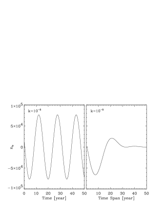
Figure 6.— Left: “instantaneous” braking index $n_{\rm b}$ as a function of time. Right: “averaged” braking index $n_{\rm b}$ as a function of the time span of the fitting. $T=15$ yr is used in both cases.

7. Summary

The results and conclusions of this work can be summarized as follows.

1. The observed braking indices of the pulsars in the H2010 sample, which span a range of more than 100 millions, are completely different from the predictions of the model of Magalhaes et al. (2012), as shown in Figure 1.

2. A significant correlation between the braking indices and characteristic ages of pulsars in the H2010 sample is found over about eight orders of magnitude, as shown in the bottom panel of Figure 2.

3. Based on the magnetic field evolution model we developed previously (Paper I), an analytical expression for the braking index is derived, as given by Equation (10). The analytically calculated correlation between the braking index and characteristic age re-produces the observed correlation well, as shown in Figure 3.

4. Our model is incompatible with the previous interpretation that the magnetic field growth is responsible for the observed small values of braking indices ($<3$) of “baby” pulsars with characteristic ages of less than $2\times 10^{3}$ yr.

5. We find that the “instantaneous” braking index of a pulsar may be different from the “averaged” braking index obtained from data. The close match between our model-predicted “instantaneous” braking indices and the observed “averaged” braking indices, as shown in Figure 4 suggests that the time spans used in the H2010 sample are usually smaller than or comparable to their magnetic field oscillation periods.

6. Our model can be tested with the existing data, by calculating the braking index as a function of the time span for each pulsar. In doing so, one can obtain all the parameters for each pulsar in our magnetic field evolution model. This is particularly important if one wants to use the long term timing data of pulsars to detect gravitational waves.

References

- Alpar et al. (2001) Alpar, M. A., Ankay, A., & Yazgan, E. 2001, ApJ, 557, L61
- Blandford & Romani (1988) Blandford, R. D., & Romani, R. W. 1988, MNRAS, 234, 57P
- Chanmugam & Sang (1989) Chanmugam, G., & Sang, Y. 1989, MNRAS, 241, 295
- Chen & Li (2006) Chen, W. C., & Li, X. D. 2006, A&A, 450, L1
- Espinoza et al. (2011) Espinoza, C. M., Lyne, A. G., Kramer, M., Manchester, R. N., & Kaspi, V. M. 2011, ApJ, 741, L13
- Ho & Andersson (2012) Ho, W. C. G., & Andersson, N. 2012, arXiv:1208.3201
- Hobbs et al. (2010) Hobbs, G., Lyne, A. G., & Kramer, M. 2010, MNRAS, 402, 1027 (H2010)
- Johnston & Galloway (1999) Johnston, S., & Galloway, D. 1999, MNRAS, 306, L50
- Livingstone et al. (2007) Livingstone, M. A., Kaspi, V. M., Gavriil, F. P., et al. 2007, Ap&SS, 308, 317
- Livingstone et al. (2006) Livingstone, M. A., Kaspi, V. M., Gotthelf, E. V., & Kuiper, L. 2006, ApJ, 647, 1286
- Lyne (2004) Lyne, A. G. 2004, Young Neutron Stars and Their Environments, IAU Symposium no. 218, (Eds., Camilo, F. & Bryan M. Gaensler, B. M.), 218, 257
- Lyne et al. (1993) Lyne, A. G., Pritchard, R. S., & Graham-Smith, F. 1993, MNRAS, 265, 1003
- Lyne et al. (1996) Lyne, A. G., Pritchard, R. S., Graham-Smith, F., & Camilo, F. 1996, Nature, 381, 497
- Magalhaes et al. (2012) Magalhaes, N. S., Miranda, T. A., & Frajuca, C. 2012, ApJ, 755, 54
- Manchester & Peterson (1989) Manchester, R. N., & Peterson, B. A. 1989, ApJ, 342, L23
- Manchester & Taylor (1977) Manchester, R. N., & Taylor, J. H. 1977, in Pulsars, ed. R. N. Manchester & J. H. Taylor (San Francisco, CA: W. H. Freeman), 281
- Menou et al. (2001) Menou, K., Perna, R., & Hernquist, L. 2001, ApJ, 554, L63
- Middleditch et al. (2006) Middleditch, J., Marshall, F. E., Wang, Q. D., Gotthelf, E. V., & Zhang, W. 2006, ApJ, 652, 1531
- Pons et al. (2012) Pons, J. A., Viganò, D., & Geppert, U. 2012, A&A, 547, A9
- Wu et al. (2003) Wu, F., Xu, R. X., & Gil, J. 2003, A&A, 409, 641
- Xu & Qiao (2001) Xu, R. X., & Qiao, G. J. 2001, ApJ, 561, L85
- Yue et al. (2007) Yue, Y. L., Xu, R. X., & Zhu, W. W. 2007, Adv. in Space Res., 40, 1491
- Zhang & Xie (2011) Zhang, S., & Xie, Y. 2012a, in ASP Conf. Ser. 451, 4519th Pacific Rim Conference on Stellar Astrophysics, ed. Shengbang Qian (San Francisco, CA: ASP), 231
- Zhang & Xie (2012) Zhang, S.-N., & Xie, Y. 2012b, ApJ, 757, 153 (Paper I)