Supersymmetric Partition Functions

and a
String Theory in 4 Dimensions

Cumrun Vafa

Jefferson Physical Laboratory, Harvard University, Cambridge, MA 02138, USA

Abstract

We propose a novel string theory propagating in a non-commutative deformation of the four dimensional space $T^{*}{\bf T}^{2}$ whose scattering states correspond to superconformal theories in 5 dimensions and the scattering amplitudes compute superconformal indices of the corresponding 5d theories. The superconformal theories are obtained by M-theory compactifications on singular CY 3-folds or equivalently from a web of 5-branes of type IIB strings. The cubic interaction of this string theory for primitive winding modes corresponds to the (refined) topological vertex. The oscillator modes of the string theory correspond to off-shell states and carry information about co-dimension 2 defects of the superconformal theory. Particular limits of a subset of scattering amplitudes of this string theory lead to the partition functions of $A_{n}$ Gaiotto theories for all $n$, compactified on $S^{4}$, i.e., to amplitudes of all Toda theories.

1 Introduction

Protected amplitudes of supersymmetric theories are frequently captured by topological theories. These are typically holomorphic quantities. In the context of supersymmetric theories arising in string theory these are computed by topological string amplitudes.

With the work of Pestun pestun on partition function of supersymmetric theories on $S^{4}$, it became clear that not only holomorphic amplitudes of supersymmetric theories can arise in partition functions but also combinations of topological/anti-topological amplitudes arise–very much along the lines of $tt^{*}$ geometry studied in the 2d context cv . This suggests that the notion of a ‘real’ topological strings exists, namely combining the usual topological string with its complex conjugate to come up with a real version. In many cases we already have all the relevant tools to study the corresponding amplitudes. The question is what is the meaning of the resulting physical system?

In this paper we study in particular the supersymmetric partition functions associated with 5d superconformal theories which arise by compactification of M-theory on singular Calabi-Yau manifolds, such as toric 3-folds dkv ; mseib ; ims ; kmv . Alternatively these are described lv by the dual type IIB network of $(p,q)$ 5-branes web . The superconformal index for these theories, i.e. their partition function on $S^{1}\times S^{4}$ is computable using topological string amplitudes on the corresponding Calabi-Yau iv .

Topological string amplitudes on toric CY threefolds can be computed using the topological vertex formalism akmv (and its refinement ikv ), which involves associating Feynamn like rules, where the relevant Feynman diagrams correspond to the geometry of the $(p,q)$ 5-brane web. This originally motivated the question of defining a quantum field theory whose amplitudes will automatically give the Feyman diagrams. However, there was a notable difference between Feynman diagrams and the amplitudes for topological strings: In the case of Feynman diagram one integrates over the internal momenta, one for each internal loop. The analog of this for the web diagram would translate to integration over the moduli space of the corresponding Calabi-Yau, which one usually holds fixed in the case of topological strings.

However as we shall see, in computing the superconformal index associated to the resulting theory, one ends up integrating over the internal loops, one integral per loop! So this major difference between the topological string diagrams and Feynman diagrams disappear and motivates the question: the Feynman diagrams are describing perturbation of which quantum theory? The main aim of this paper is to propose an answer to this question. We propose that these Feynman diagrams correspond to scattering amplitudes of a string theory propagating in 4-dimensional non-commutative version of space-time $T^{*}{\bf T}^{2}$. The choice of the 5d superconformal theory translates to the choice of the winding sectors of the string scattering states and the choice of the transverse position of the winding string on ${\bf T}^{2}$ translate to scattering momenta of the Feyman diagrams which are chemical potentials for global symmetries of the 5d superconformal theory. Moreover the oscillation modes of the string are off-shell states and they enjoy a natural cubic vertex structure, which is the (refined) topological vertex. The off-shell states capture amplitudes associated with the codimension 2 defect operators of the 5d superconformal theory. The natural Wick rotations of this theory suggests a signature $(2,2)$ for the space-time, and raises the question of relation of this string theory to $N=2$ strings ov .

The corresponding 5d superconformal theories reduced on a circle give a rich class of ${\cal N}=2$ superconformal theories, which include in particular all the $A_{n}$ Gaiotto theories gaiotto . Thus the partition functions of these theories, which are conjectured to be related to Toda theories, get related to specific scattering amplitudes of the string theory we propose, where the choice of the scattering states in the string theory, determines the choice of the Gaiotto theory. It would also be interesting to investigate the properties of the more general class of 4d ${\cal N}=2$ theories that we obtain, whose partition functions are computed by the string theory we propose.

The organization of this paper is as follows: In section 2 we review the construction of 5d conformal theories obtained from M-theory on toric manifolds (including some which admit singular toric action) or equivalently type IIB on a web of $(p,q)$ 5-branes (which could end on 7-branes). In section 3 we discuss how one can use topological strings to compute superconformal indices for these theories. In section 4 we propose the string theory in 4 dimensions, and in section 5 we end with some open questions.

2 Toric Geometry, (p,q) 5-brane Web and 5d Superconformal Theories

It is believed that compactifying M-theory on singular Calabi-Yau 3-folds can lead to superconformal theories in 5 dimensions involving interacting massless particles and tensionless strings wphase ; dkv ; mseib ; ims . It is also known lv that this is dual to a web of $(p,q)$ 5-branes web . In this section we review some basic features of these conformal theories, reformulated in a way which will be most useful to us in this paper.

A toric Calabi-Yau 3-fold is captured by the geometry of which cycles of a ${\bf T}^{2}$ shrink and what their intersection geometry is. Moreover the duality between M-theory on ${\bf T}^{2}$ and type IIB on $S^{1}$ allows us to convert a locus with a $(p,q)$-cycle of ${\bf T}^{2}$ shrinking with a $(p,q)$ 5-brane of type IIB. Thus the geometry of toric Calabi-Yau 3-folds can be captured by a web of $(p,q)$ 5-branes. Each such 5-brane fills the 5-dimensional space-time and has 1-dimension extended along a straight line in ${\bf R}^{2}$. The intersecting structure of the $(p,q)$-branes in ${\bf R}^{2}$ forms a web $W\subset{\bf R}^{2}$. We can view $W$ as oriented, where the orientation on the web distinguishes $(p,q)$ brane from a $(-p,-q)$ brane. Charge conservation of the $(p,q)$ 5-brane implies that $\sum_{i}(p_{i},q_{i})=0$ for each junction (vertex) where $(p,q)$ 5-branes meet. The generic junctions of the $(p,q)$ 5-branes are cubic. Moreover, if we introduce the inner product between $w=(p,q)$ 5-branes, given by

$$\langle w_{1},w_{2}\rangle=\langle(p_{1},q_{1}),(p_{2},q_{2})\rangle=p_{1}q_{2}-q_{1}p_{2},$$

the generic cubic vertex has the property that

$$\langle w_{1},w_{2}\rangle=\pm 1$$

Figure 1: An example of $(p,q)$ web with $N=6$ external lines and $g=3$ internal loops.

Figure 2: A breathing mode corresponds to changing the web, without moving the external lines. There is one breathing mode per internal loop.

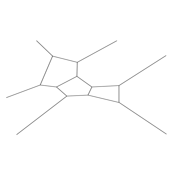
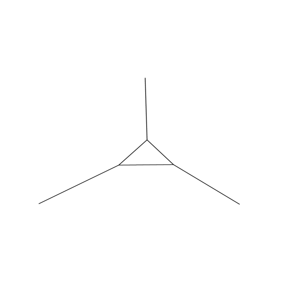
Properties of these theories are nicely captured by the properties of the branes web , which we now review. To balance the tension between the branes at the junctions, the orientations of $(p,q)$ 5-branes should be such that there is no force at the vertex. This is automatically the case if the $(p,q)$ brane is directed along the line $(p+q\tau)$ where $\tau$ is the type IIB coupling constant. Up to a rotation in $R^{2}$ this is the most general solution for balancing the tensions. Since $\tau$ will not play a role in this paper, for simplicity of exposition we take $\tau=i$, in which case the $(p,q)$ 5-brane is directed along a line with slope $q/p$. For an example of a $(p,q)$ web see Fig.1.

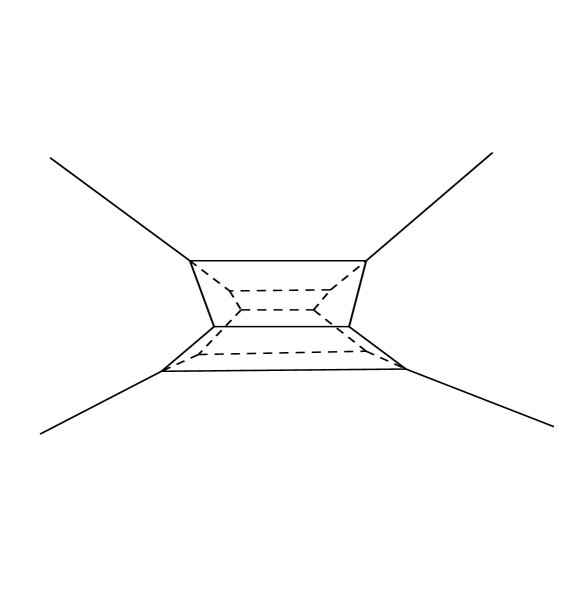
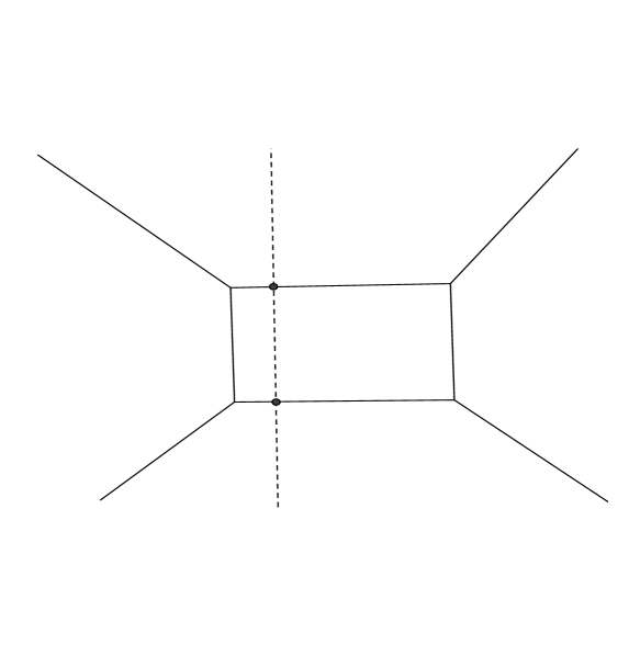
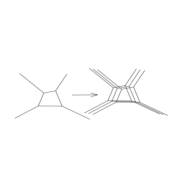
Any web $W$ will have a number of $(p,q)$ branes which are semi-infinitely extended along ${\bf R}^{2}$. These we will call the ‘external lines’ of the web. The rest of the 5-branes will be called ‘internal’. Moving the external lines in ${\bf R}^{2}$ requires infinite energy compared to the internal lines. Thus the degree of freedom of moving the external lines are non-normalizable and can be viewed as ‘mass parameters’ of the theory. The internal lines correspond to normalizable modes. Let us fix the mass parameters, and thus the position of external lines. Of course we cannot move the internal lines arbitrarily. First, the branes can only move parallel to themselves, to preserve tension. Secondly, the external lines are fixed. It is easy to see that for each primitive closed cycle (loop) in the web diagram, there is one mode which corresponds to the ‘breathing mode’ of the loop (see Figure 2). This is in perfect agreement with the M-theory picture, as each closed loop corresponds to a 4-cycles in the toric Calabi-Yau, and the primitive loops form a basis for 4-cycles. Moreover the corresponding breathing mode of the loop is the scalar corresponding to the normalizable Kähler mode. The internal lines of the web $W$ correspond to 2-cycles of the Calabi-Yau, though they are not independent classes. We shall denote by $N$ the number of external lines and by $g$ the number of primitive loops of the web. The theory will have a $U(1)^{g}$ gauge symmetry and the breathing modes are the real scalars in the corresponding vector multiplets. Note that we can view the web as a Feynman diagram with $N$ external lines, describing the scattering of $N$ particles at $g$-th loop order. In general, for fixed external lines, as we change the Kähler classes, the topology of the web may change, though generically it will still have $g$ primitive loops. From the viewpoint of Calabi-Yau this corresponds to transitions from one Calabi-Yau to another.

2.1 Integral convex polygon associated to the web

Consider a web of 5-branes with $N$ external lines corresponding to classes $w_{i}$ where we orient the external lines towards infinity. Then by the brane charge conservation we know that

$$\sum_{i=1}^{N}w_{i}=0.$$

Using the external lines we can define an integral convex polygon $P$ in the following way: Consider an infinite radius circle and order $w_{i}$ in increasing order as we go around the circle in a counter-clock wise direction. If there are several parallel $w_{i}$, they will clearly be one after the other in this sequence.

Using this data we can define an integral convex polygon $P$. This is a polygon whose vertices are on integral points of ${\bf R}^{2}$. Furthermore the edges of $P$ passes through $N$ integral points. Let $a_{j}$ correspond to the $j$-th integral point of $P$. This polygon is defined (up to an overall shift in the lattice) by the condition that

$$a_{j+1}-a_{j}=iw_{j}$$

where $iw_{j}=i(p_{j},q_{j})=(-q_{j},p_{j})$. Note that since $\sum_{i}w_{i}=0$ we learn that $a_{N+1}=a_{1}$. In other words we have a closed polygon passing through $N$ integral points. The fact that $P$ is convex follows from the fact that the angle that $w_{i}$ makes with the positive $x$-axis is increasing (in the counter-clockwise sense). The number of integral points on each edge of $P$ minus one is the number of parallel 5-branes in that direction.

Figure 3: An example of a $(p,q)$ web with $N=4$ external lines and $g=2$ internal loops. The convex outer polygon has 4 sides and its triangulation is dual to the web.

Even though it is not obvious, $g$ is the number of integral points in the interior of $P$. Moreover the number of internal points $g$ can be computed according to (Pick’s theorem):

$$g=A-{N\over 2}+1={1\over 2}\sum_{i<j}\langle w_{i},w_{j}\rangle-{N\over 2}+1$$

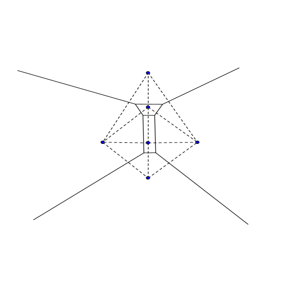
where $A$ is the area of $P$. In fact if we consider a generic web with the asymptotic states fixed by a polygon, and view the interior points as vertices (leading to a ‘grid diagram’) and triangulate them, each triangulation corresponds to a choice of web diagram with fixed external lines. The web is dual to this triangulation. In this picture, each face of the triangulation corresponds to a cubic vertex of the web and each edge of the web is orthogonal to an edge of the triangulation. See Figure 3.

If we compactly this 5 dimensional theory on a circle we obtain an ${\cal N}=2$ theory in 4 dimensions. The $(p,q)$ web of 5-branes can get dualized to an M-theory description involving M5 branes wrapping an SW curve. Equivalently, in the geometric picture of the M-theory on toric geometries we are led to type IIA on toric manifolds which is mirror to type IIB on the 3-fold with geometry $F(X,P)=uv$ where the curve $F(X,P)=0$ is the SW curve and is given by

$$\Sigma:\qquad F(X,P)=\sum_{m,n\in P}a_{mn}X^{m}P^{n}=0$$

where ${m,n}$ are integral points inside, or on the boundary of $P$. The $X,P$ are ${\bf C}^{*}$ variables and we sometimes also write them as

$$X={\rm exp}(x)={\rm exp}(-\tau_{x}+i\theta_{x})$$

$$P={\rm exp}(p)={\rm exp}(-\tau_{p}+i\theta_{p})$$

$X,P$ can be explained in the type IIB parameterization as follows: The $(\theta_{x},\theta_{p})$ can be naturally identified with the F-theory elliptic fiber $T^{2}$ and $(\tau_{x},\tau_{p})$ denotes the ${\bf R}^{2}$ on which the web of $(p,q)$ 5-branes were stretched. The $a_{mn}$ are complex parameters which parameterize the Coulomb branch of the theory if $(m,n)$ is one of the $g$ interior points of $P$. If $(m,n)$ is on the boundary of $P$, $a_{mn}$ is a mass parameter of the theory. The SW differential can be identified with

$$\lambda_{SW}=pdx.$$

The SW curve $\Sigma$ can be identified as the fattened up version of the web diagram. Moreover if $(m_{1},n_{1})$ and $(m_{2},n_{2})$ correspond to two successive points on the boundary of $P$ the cylinder associated with that edge comes from the part of the polynomial given by

$$a_{m_{1}n_{1}}X^{m_{1}}P^{n_{1}}-a_{m_{2}n_{2}}X^{m_{2}}P^{n_{2}}\sim 0$$

leading to the cylinder given by

$$X^{m_{2}-m_{1}}P^{n_{2}-n_{1}}=a_{m_{1}n_{1}}a^{-1}_{m_{2}n_{2}}$$

which corresponds to the $(p,q)$ 5-brane associated with $w=(n_{2}-n_{1},m_{1}-m_{2})$.

2.2 Adding 7-branes

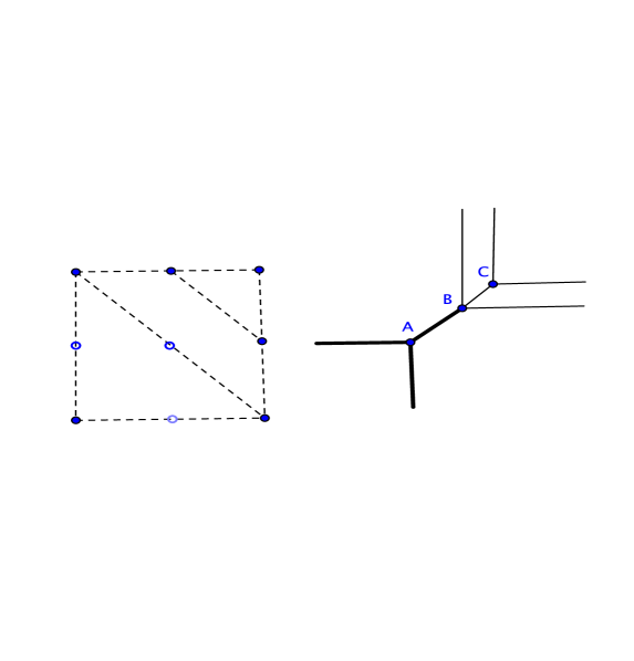
It is also possible to add 7-branes to this story, where the 5-branes can end on. This has been recently revisited in tach . These will correspond to M-theory compactified on non-toric Calabi-Yau which admit singular torus actions. This construction will allow us to also discuss manifolds such as ${\bf P}^{2}$ blown up at 8 points inside a Calabi-Yau in the context of webs. In this context it is natural to put the 7-branes at infinity in ${\bf R}^{2}$. Thus the external lines will be grouped according to which 7-brane it ends on. Sometimes this geometry is depicted by adding white dots to the diagram tach . The white dots signify the grouping of the 5-branes. In particular the 5-branes ending on the same 7-brane are dual to edges which are separated by white dots. See Figure 4. The rules of what type of vertices the 5-branes with multiplicity can have, has been worked out and we review them later in section 4.

Figure 4: An example of grouping 5-branes according to which 7-branes they end on. The dual grid contains white dots to depict the corresponding grouping. The vertices of the web correspond to faces of the grid. Vertex A corresponds to the bigger triangle. Vertex B the trapezoid and vertex C to the small triangle. The thicker edges of the web correspond to two 5-branes.

2.3 Introducting defects

Figure 5: The D3 branes (or Lagangian branes in the M theory setup), are suspended between a 5-brane at infinity (denoted by a dashed line) and the web. The D3 branes are perpendicular to the plane ending on the web at one of the two dots.

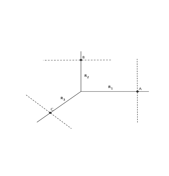
It is also possible (and important) to introduce defect probes in this theory. In the M-theory setup on Calabi-Yau, they correspond to wrapping a number of M5 branes on a special Lagrangian subspace MV , filling a 3-dimensional subspace of space-time. This can be viewed as a codimension 2 defect in the 5-dimensional theory. In the language of $(p,q)$ 5-brane web, they correspond akv to introducing D3 branes which fill a 3-dimensional part of 5d space-time and correspond to a semi-infinite line in the orthogonal direction to the ${\bf R}^{2}$ plane of the web, which end on an edge on the 5-brane. To fix a class of such defect probes it turns out to be natural to view the semi-infinite D3 brane probe to be a finite segment that ends on a spectator $(p,q)$ 5-brane which is placed infinitely far above the plane of the web (see Figure 5). In the geometric language introducing the spectator 5-brane at infinity corresponds to choosing a compactification of the special Lagrangian which the M5 brane wraps.

If one compactifies this theory on a circle down to 4 dimensions, the resulting defect will correspond to a surface operator of the ${\cal N}=2$ theory. In the context of webs which give rise to gauge theories some of these probes can be viewed as surface operators of the type studied in gw and connected to this picture in wk ; dg . They correspond to choosing a collection of points on the SW curve, where the D3 brane intersects the web.

In this context as we consider the normalizable deformations of the web, i.e. the breathing modes associated with the closed loops in the web, the spectator 5-branes at infinity do not move, but the D3 brane suspended between the spectator 5-brane and the web slide along the spectator brane in unison with the breathing mode, so as to continue ending on the web. This defines the class of the defect operators as we give expectation values to the fields. It is in this context that it becomes clear that we need the spectator $(p,q)$ 5-brane at infinity to actually define the defect operator. Different choices of the spectator 5-brane lead to different defect operators. Needless to say we can introduce as many defect probes and as many D3 branes suspended between them and the web, as we wish. The geometry of where the D3 brane probe ends on the web, defines different types of defect operators, which map, upon reduction to 4d in the gauge theory case, to the different types of defects allowed in gauge theory.

2.4 5d Superconformal Points

Figure 6: At the conformal point the web collapses to rays passing through one point.

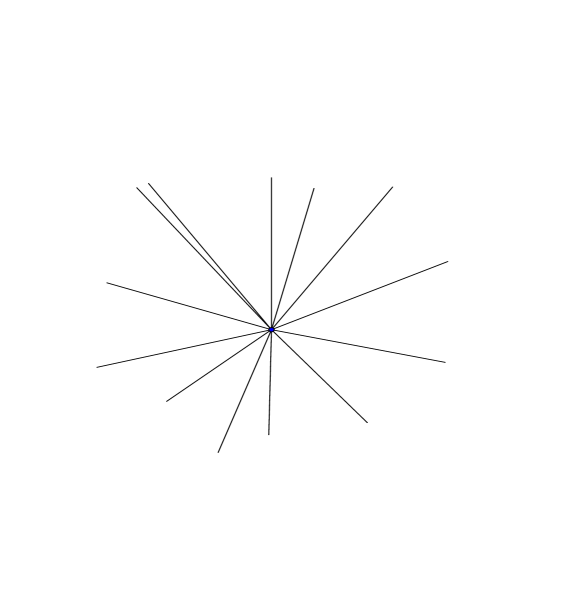
When 4-cycles in the CY shrink to zero size, we get tensionless strings by wrapping M5-branes over them. In the type IIB setup the tensionless string corresponds to D3 branes wrapping the minimal cycles and ending on the (p,q) 5-branes. In addition M2 branes wrapping over the corresponding 2-cycles inside the 4-cycle is massless. We thus get a collection of interacting massless particles and tensionless strings which suggests we have a conformal fixed point. For each web, with at least 1 internal integral point (i.e. $g\geq 1$) we thus end up with a non-trivial conformal theory where all the internal loops vanish. In this limit the web collapses to $N$ semi-infnite lines passing through the same point (where some semi-infinite lines may have multiplicity, associated to external 5-branes with the same $(p,q)$). See Figure 6. We can further group these according to which parallel ones end on the 7-brane. It is natural to conjecture that for each such configuration there is a unique superconformal theory in 5 dimensions. Thus we can associate to each integral convex polygon $P$, with possible white dots which signify the grouping of the same type $(p,q)$ branes, a superconformal theory. Two convex integral polygons define the same superconformal theory if they can be mapped to one another by translation on the integral lattice, as well as an $SL(2,Z)$ change of basis.

Note that the number of mass parameters for this conformal theory is $N-3$ where $N$ is the number of (black) integral points on the boundary of the polygon (i.e. external lines). This is because we have one mass parameter corresponding to moving each group of external lines, except that a two parameter subspace of this simply corresponds to moving the intersection point of the lines on ${\bf R}^{2}$ and does not change the theory. We first need to say more precisely how the masses are parameterized: For each brane given by a vector $w\in H_{1}(T^{2},{\bf Z})$ we choose a $v\in H_{1}(T^{2},{\bf Z})$ such that $\langle w,v\rangle=1$. $v$ is unique up to shifting it by an integer multiple of $v$:

$$v\rightarrow v+nw$$

Each such choice of $v$ we will call a ‘framing’ associated to the brane $w$. Consider moving the brane $w$ along ${\bf R}^{2}$. We parameterize the motion by a real number (mass) $m\in{\bf R}$ multiplied by $v$. In other words, we move every point of $w$ on ${\bf R}^{2}$ by $mv$. Note that the choice of framing is irrelevant for this motion as different framings correspond to shifting the brane parallel to itself which does not change the brane.

We now show that if we parameterize the $m_{i}$ corresponding to movement of the branes from the superconformal point (i.e. where $m_{i}=0$ correspond to the superconformal point) then they are not independent. In particular

$$\sum_{i=1}^{N}m_{i}=0.$$

To show this we will first show this for three primitive brane junctions. Consider the case with three primitive 7-branes, $w_{1},w_{2},w_{3}$ with

$$\sum w_{i}=0\quad and\quad\langle w_{1},w_{2}\rangle=\langle w_{2},w_{3}\rangle=\langle w_{3},w_{1}\rangle=1$$

Note that by an $SL(2,Z)$ transformation we can take $(w_{1},w_{2},w_{3})=((1,0),(0,1),(-1,-1))$. We can conveniently choose the framings

$$v_{1}=w_{2},v_{2}=-w_{1},v_{3}=w_{1}$$

If we move $w_{1}$ by $m_{1}v_{1}=(0,m_{1})$ and $w_{2}$ by $m_{2}v_{2}=(-m_{2},0)$ the intersection point between $w_{1}$ and $w_{2}$ branes will have moved by $(-m_{2},m_{1})$. Now the $w_{3}$ brane will have to be moved to pass through it. Indeed if we shift $w_{3}$ by $m_{3}v_{3}=(-m_{1}-m_{2})(1,0)$ then it passes through it because $(-m_{2},m_{1})-(-m_{1}-m_{2},0)=m_{1}(1,1)$. We thus learn that consistency of the brane configuration requires that

$$m_{1}+m_{2}+m_{3}=0$$

Now let us consider the general web in a generic position . We can associate to each edge a mass parameter $m_{i}$. The generic web will have cubic vertices which as we have just shown require $\sum m_{i}=0$ at each vertex. Thus the conservation of $m_{i}$ implies that the sum of the $m_{i}$ over all the external lines vanishes:

$$\sum_{i=1}^{N}m_{i}=0,$$

which is what we wished to show. Moreover, we can show that two combination of mass parameters are redundant. In fact let $u_{1},u_{2}$ be a basis for $H_{1}(T^{2},{\bf Z})$. Translations of ${\bf R}^{2}$ by $u=r_{1}u_{1}+r_{2}u_{2}$ will shift all the masses according to

$$m_{i}\sim m_{i}+\langle w_{i},u\rangle$$

Thus out of $N$ potential mass parameters we are left with $N-3$ independent parameters.

Upon compactification on a circle the mass parameters become complexified and as we have discussed they are captured by the ratio of the coefficients associated with the boundary monomials of $P$. In particular to each external line $w$ we associate the exponentiated mass parameter

$$M_{w}=exp(-m_{w}+i\theta_{w})$$

Furthermore, recall that each $w$ is associated with a boundary edge $w=-i(m,n)=(n_{2},-m_{2})-(n_{1},-m_{1})$ of $P$ and we get the identification

$$M_{w}=a_{m_{1}n_{1}}/a_{m_{2}n_{2}}$$

The analog of the mass condition $\sum m_{i}=0$ gets mapped to

$$\prod_{w\in\partial P}M_{w}=1$$

which is automatic. Moreover rescaling $X\rightarrow\alpha X$ and $P\rightarrow\beta P$ shifts

$$M_{w}\rightarrow M_{w}\ \alpha^{m}\beta^{n}$$

which gets rid of two additional complex mass parameters. In other words the angular part of the mass parameters $\theta_{w}$ also satisfy the constraint

$$\sum\theta_{w}=0$$

and

$$\theta_{w}\sim\theta_{w}+\langle w,u\rangle$$

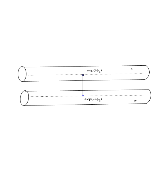
These can be interpreted as follows. Let us consider one of the external lines given by $w$. For simplicity of exposition let us take the external line corresponding to $w=(1,0)$. This corresponds to tube spanned by $X$. In general we can parameterize the SW curve by choosing $X$ as the local coordinate. In this way $P$ can be viewed as a holomorphic function $P(X)$ along the tube. More precisely we can view $p(x)dx$ as a 1-form along the tube which gives the data of the geometry. For $|X|>>1$ the transverse position of the tube approaches a constant on the $P$ tube given by

$$P=M_{w}$$

Figure 7: An external line is characterizes by a winding $w$ on ${\bf T}^{2}$. The transverse position of the string, as measured from some base point $B$ on ${\bf T}^{2}$ corresponds to $\theta_{w}$.

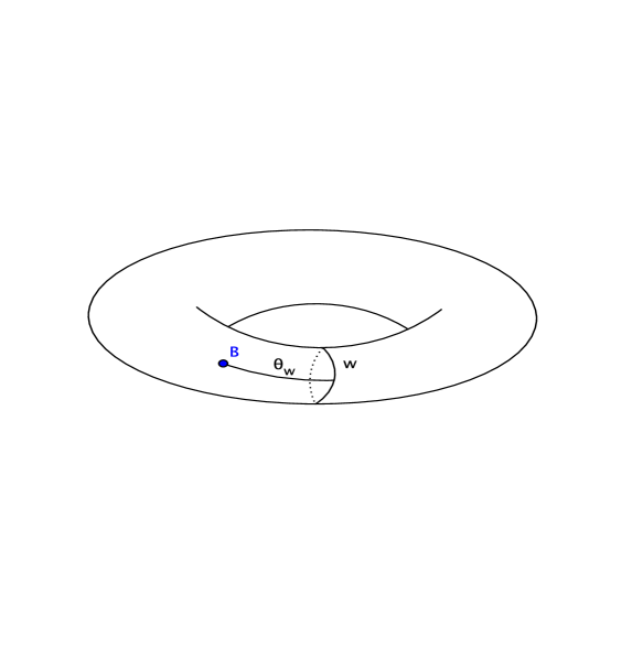
Changing $m_{w}$ corresponds to moving the position of the transverse point of the tube along $\tau_{p}$ and changing $\theta_{w}$ corresponds to rotating the position of the tube in the angular direction. Note that if we project this tube to the ${\bf T}^{2}:(\theta_{x},\theta_{p})$, it is wrapped around $\theta_{x}$ at a position given by $\theta_{p}=\theta_{w}$. The angular part of the framing of a tube depends on which base point we measure the position of $\theta_{x}$ from. Shifting the base point on ${\bf T}^{2}$, where we measure $\theta_{w}$ corresponds to the degree of freedom of shifting the angular part of the masses by two parameters. See Figure 7.

3 Topological Strings and 5d Superconformal Indices

Consider M-theory on a Calabi-Yau threefold $K$. In addition compactify further on $S^{1}\times TN$ where $TN$ denotes Taub-NUT. The circle product is twisted: as we go around $S^{1}$ we rotate the two complex planes of $TN$ by

$$(z_{1},z_{2})\rightarrow(qz_{1},q^{-1}z_{2})$$

If the Calabi-Yau is non-compact as in toric cases, and has an extra geometric $U(1)$ rotation corresponding to R-symmetry, we get a refinement of this by allowing independent rotations

$$(z_{1},z_{2})\rightarrow(q_{1}z_{1},q_{2}^{-1}z_{2})$$

and rotating the internal geometry by a $U(1)$ rotation given by $q_{1}q_{2}^{-1}$. The partition function of M-theory for this geometry is a definition of topological string dvv :

$$Z_{M}(K\times S^{1}\times_{(q_{1},q_{2})}TN)=Z^{top}(K,q_{1},q_{2})$$

A series of arguments dvv relate this definition to the usual definition of A-model topological string when $q_{1}=q_{2}=q=exp(i\lambda)$, where $\lambda$ is the topological string coupling constant. In this paper for simplicity we sometimes specialize discussion to this case, though the generalization of the amplitudes and methods for computation of refined topological strings are also known.

The topological string partition function for toric geometries (which correspond to webs with multiplicity 1 on each edge) can be computed using topological vertex formalism akmv (and its refinement ikv –see also awata ) which was inspired by the large $N$ dualities of topological strings GV .

As discussed already, the Calabi-Yau on toric geometries can be represented by a web $W$ of $(p,q)$ 5-branes. The generic such web has cubic vertices. The topological vertex formalism associates a Young diagram, or equivalently a finite representation $R$ of $U(\infty)$ to each internal line. Furthermore to each edge one associates a ‘propagator factor’ given by $Q^{n(R)}={\rm exp}(-n(R)t)$ where $n(R)$ is the number of boxes of $R$, $Q=e^{-t}$ and $t$ is the complexified length of the edge (i.e. the integral $t=\oint_{tube}pdx$). Note that to obtain finite amplitudes we need to put trivial representation on the external lines, since $Q_{external}=0$ due to infinite length of external lines. Moreover for each cubic junction one introduces a vertex $C(R_{1},R_{2},R_{3};q_{1},q_{2})$. The partition function is computed by summing over all representations $R$ for the internal edges.

The fact that each edge is associated with a representation $R$ is reminiscent of the oscillator mode of a single chiral boson or a complex chiral fermion. This analogy proved important in explanation of the structure of the topological vertex akmv ; IH , as we will now review. Consider a tubular geometry of the web. Let us assume, with no loss of generality, that the tube corresponds to wrapping the ${\bf C}^{*}$ direction corresponding to $X$. The embedding of this tube in ${\bf C}^{*}\times{\bf C}^{*}$ can be characterized by how $P$, the position on the orthogonal ${\bf C}^{*}$, varies over the tube parameterized by $X$. Noting that the normal direction $p$ belongs to the cotangent of $x$-space, it is natural to describe the normal deformation as being a 1-form in the $x$-space. We thus consider the normal deformation as

$$pdx=p_{cl}(x)dx$$

where $p_{cl}(x)dx$ can be read from the classical geometry of the mirror curve $F(X,P)=0$, by solving $p$ in terms of $x$. It is natural to ask about fluctuations of this classical geometry, in a holomorphic way. This in particular is parametrized as

$$p=p_{cl}(x)+\sum_{n}\alpha_{n}X^{n}=p_{cl}(x)+\sum_{n}\alpha_{n}{\rm exp}(-n(\tau_{x}+i\theta_{x}))$$

given that $pdx$ is a 1-form, and it is chiral, it is natural to identify it with a chiral bosonic current:

$$pdx=\partial\phi$$

which satisfies ${\overline{\partial}}\partial\phi=0$. In fact more is true: The radius of the boson (for the unrefined topological string) is such that the boson is equivalent to a complex fermion and we can write

$$\partial\phi=\psi^{*}\psi$$

For this to be true, the radius of $\phi$ should be 1, such that $\psi={\rm exp}(i\phi)$. This turns out to be true as explained in IH . The basic idea is that the $\psi$ corresponds to creation operator for the Lagrangian brane in the Calabi-Yau, or in the type IIB setup as the D3 brane ending on the web. In other words if we add a codimension 2 defect to our theory, this is equivalent to insertion of $\psi$ at a particular point on the curve. The period of $\phi$ is precisely correct to capture the charge of the brane ending on the web.

Figure 8: Topological vertex can be viewed as the partition function of topological string in the presence of defects introduced by branes which end on the web at $(A,B,C)$. The excitations $(R_{1},R_{2},R_{3})$ on the legs are created by them.

The introduction of defects plays a key role in the definition of topological vertex akmv . In fact the topological vertex can be viewed as the study of the configuration dual to ${\bf C}^{3}$ where we have introduced three sets of defect probes, one for each edge of the associated web. In this way the branes suspended between the spectator 5-brane and the web, create excitations on each of the corresponding legs of the web, whose amplitude is given by $C_{R_{1}R_{2}R_{3}}$. See Figure 8.

This structure naturally explains why each edge is labeled by a Young diagram, which is naturally identified with bosonic oscillator fock space (or equivalently $U(1)$ neutral states in a complex fermionic fock space) where the propagator is $Q^{L_{0}}$. However if this description is correct then one would expect that the topological vertex is simply the vertex associated with a chiral boson on thrice puncture sphere. This is almost true! However the topological vertex depends on the couplings $q_{i}$. The way this appears is that $\psi(x)$, the brane creation operator, is not an ordinary fermion on a Riemann surface $F(X,P)=0$, but rather $x,p$ do not commute when acting on $\psi$. In particular in the case $q_{1}=q_{2}^{-1}={\rm exp}(i\lambda)$

$$[x,p]=i\lambda$$

We view $F(X,P)=0$ (with suitable ordering of $x,p$) as an operator which annihilates $\psi$

$$F(\hat{X},\hat{P})\psi=0$$

and this leads to Ward identities which fix the cubic vertex IH . The appearance of this structure was further explained in sulk using the M-theory definition of topological strings, and by applying various dualities to it. In particular it was shown there that the topological strings partition function gets mapped to the partition function of type IIA strings for the flat background on ${\bf R^{3}}\times{\bf C}^{*}\times{\bf C}^{*}\times{\bf R^{\prime}}^{3}$, where a D6 brane wraps ${\bf C}^{*}\times{\bf C}^{*}\times{\bf R^{\prime}}^{3}$ and a D4 brane wraps ${\bf R}^{3}\times\Sigma$, where $\Sigma\subset{\bf C}^{*}\times{\bf C}^{*}$ is given by $F(X,P)=0$. Notice that the D4 and D6 brane intersect over $\Sigma$ and the strings stretched between them leads to a complex chiral fermion on $\Sigma$. Moreover an NS B-field is turned on over the D6 brane given by $B=dx\wedge dp/i\lambda$. Only the holomorphic part of this was relevant for the topological string, but of course reality of $B$ demands that

$$B={1\over i\lambda}[dx\wedge dp-d{\overline{x}}\wedge d{\overline{p}}]$$

This B-field makes the D6 brane non-commutative sw with non-commutativity

$$[x,p]=i\lambda$$

Moreover the D4-D6 strings form a representation of this non-commutative algebra kw , making the fermions behave as a D-module, exactly as was originally found for the topological vertex.

3.1 A purely 4 dimensional perspective

From the description of the topological string amplitudes in terms of D4 and D6 branes discussed in the previous section, as well as the description given in the case of the 5-brane web, it is clear that the main object of interest takes place in the 4-dimensional space

$$M={\bf C}^{*}\times{\bf C}^{*}$$

Getting rid of the ${\bf R^{3}}\times{\bf R^{\prime}}^{3}$ part of the type IIA string, the D6 brane is replaced by a D3-brane wrapping all of $M$, and D4 brane is replace by a D1-brane wrapping a holomorphic curve $\Sigma$ in $M$. Moreover there is a $B$-field turned on in $M$ which is

$$B={1\over\lambda}{\rm Im}\Omega$$

where $\Omega$ is the holomorphic 2-form on $M$ given by

$$\Omega={dX\wedge dP\over XP}=dx\wedge dp$$

Thus we have one 4-dimensional and one 2-dimensional brane in $M$. We are thus naturally led to ask if there is a theory on $M$ which is equivalent to topological string associated to toric Calabi-Yau. The answer turns out to be yes! Indeed we can consider topological strings directly on $M$. Since $M$ is hyperKähler the branes can be distinguished in more refined ways, depending on which complex structure one considers. The D3 brane, together with the $B$ field, turns out to be a co-isotropic brane of the type introduced in ko and studied in the hyperKähler context in kw . For a co-isotropic brane we need $k\wedge k=B\wedge B$ and the $k\wedge B=0$, both of which are easily checked to be true, where $k$ is the Kähler form which we take to be

$$k={i\over\lambda}(dx\wedge d{\overline{x}}+dp\wedge d{\overline{p}}).$$

In fact this is a ‘canonical co-isotropic brane’, or ‘cc brane’ (since the $B$ field is identified with the imaginary part of the canonical holomorphic 2-form on $M$). This is an $(A,B,A)$ brane distinguishing its brane type relative to the three different complex structures. The brane associated with $\Sigma$ is a holomorphic brane relative to the usual complex structure, but corresponds to a Lagrangian brane relative to the other two complex structures (as real and imaginary parts of $\Omega$ vanish on it), and it is thus called a $(B,A,A)$ brane. In this setup, one case ask what is the nature of the string stretched between the 4-brane and the 2-brane and that turns out to be a chiral fermion kw . Moreover the canonical co-isotropic brane has a non-commutativity induced by $B$ and fermions become what is called a D-module for this non-commutative algebra exactly as was expected for the topological strings. We can summarize this by the statement that the partition function of the topological string on toric Calabi-Yau 3-fold is the same as the partition function of topological string on the 4-manifold $M$ with one cc brane filling $M$ and one $(B,A,A)$ 1-brane wrapping the curve $\Sigma$ mirror to the toric 3-fold, where the coupling constant of string theory is inversely proportional to the strength of the B-field on $M$.

3.2 Superconformal Index

The index of ${\cal N}=1$ superconformal theories in 5d, can be computed by studying the partition function of the theory on $S^{1}\times S^{4}$ where we twist $S^{4}$ by rotations $q_{1},q_{2}$ as we go around $S^{1}$. Moreover we do an R-symmetry rotation by $(q_{1}q_{2})^{-1}$ For some examples of computation of superconformal index see kimyeong . This can be connected with topological strings setup where roughly speaking we can view $S^{4}$ as gluing two copies of $TN$ and the circle actions on the two $TN$’s are opposite. This can be viewed as the partition function of the resulting $4d$ theory on $S^{4}$. In this context, as studied in pestun we know that the partition function is given by the integral of the form

$$Z_{S^{4}}=\int\prod_{i}d{a_{i}}\big{|}Z^{Nek.}(a_{i};M_{j},q_{1},q_{2})\big{|}^{2}$$

where the integral is over a Lagrangian subspace of the electric Coulomb parameters $a_{i}$, and $M_{j}$ denote the mass parameters and coupling constants. On the other hand the Nekrasov partition function for theories coming from 5d, is believed to be equal to the refined topological string partition function. We thus learn that

$$Z_{S^{4}\times S^{1}}=\int\prod_{i}da_{i}\big{|}Z^{top}(a_{i};\theta_{j},q_{1},q_{2})\big{|}^{2}$$

This structure is explained in iv . As discussed there, the integration cycle of moduli of the Coulomb branch is identified with the $a_{i}=\theta_{i}$, i.e., the compact imaginary part of Coulomb branch parameters and $\theta_{j}$ above denotes the imaginary part of mass parameter, which is chemical potential associated with the corresponding global $U(1)$ symmetry. We have one such parameter for each closed loop in the web diagram. What this means in the topological vertex formalism is that, we will have two Young diagrams on each leg, one for the topological theory and one for the anti-topological theory. This can be interpreted as making the chiral boson (or equivalently the chiral fermion) living on $\Sigma$ become a non-chiral boson (or fermion). Moreover the propagators are now

$$Q^{L_{0}}\ {\overline{Q}}^{\overline{L}_{0}}$$

Furthermore for each edge which is part of the loop we integrate over the angular part of the breathing mode. In particular for each loop with integral variable $\theta$ we get a factor

$$\int...\ \prod_{i\in\ edge\ in\ loop}{\rm exp}(i\theta(L^{i}_{0}-{\overline{L}^{i}_{0}}))\ d\theta...$$

This is similar to what we encounter in string diagrams, with two major differences: The propagators are associated to real integrals, which corresponds to twisting the tube rather than lengthening it (the real part of external mass parameters set the length of the propagator tubes). Secondly the angular integral does not project to level matching condition for left and right movers for each edge, because the integral includes all edges in a given loop. This integral projects to the condition that the sum of left-moving oscillator numbers for all edges in a given loop is equal to the corresponding sum over the right-moving oscillator numbers.

As already discussed the superconformal theories we have considered are parameterized by the following data: We choose $N$ elements each of which is an element $w_{i}\in H_{1}({\bf T}^{2},{\bf Z})$. More precisely we choose a specific straight winding mode in each given homology class, which comes in addition with an angle corresponding to moving the winding mode parallel to itself, which we denote by $\theta_{i}$. We denote the corresponding superconformal index for this theory by

$$I(w_{1},\theta_{1},...,w_{N},\theta_{N};q_{1},q_{2})$$

As we have already noted $I$ vanishes unless the following conservation laws hold:

$$\sum_{i=1}^{N}w_{i}=0,\qquad\sum_{i=1}^{N}\theta_{i}=0$$

In other words

$$I(w_{1},\theta_{1},...,w_{N},\theta_{N};q_{1},q_{2})=\delta(\sum w_{i})\delta(\sum\theta_{i})f(w_{i},\theta_{i};q_{1},q_{2})$$

We have seen evidence of a new string theory in 4-dimensions. We now collect these evidences and propose a new string theory in 4 dimensions.

4 A String Theory in 4 Dimensions

The string theory we propose propagates in the 4-dimensional space

$$M={\bf C}^{*}\times{\bf C}^{*}=T^{*}{\bf T}^{2}.$$

This space comes equipped with a natural flat Kähler metric. This would be viewed as the Euclidean version of the theory. There is no natural $(3,1)$ signature version of this theory, due to the importance of symplectic/holomorphic structure in this geometry. The closest analog of Wick rotation in this theory, due to its complex structure, would correspond to changing the signature of the metric in the ${\bf R}^{2}$ in the cotangent directions of $M$, $(\tau_{x},\tau_{p})$. In this way each of the asymptotic tubes will in fact be stretched in the usual $1+1$ signature geometry. Thus the Wick rotation would be associated to a $(2,2)$ signature space, as is the case with $N=2$ strings ov .

We will now describe its physical on-shell states, its off-shell states, and its scattering amplitudes. We will then suggest some steps in how one can come up with a more direct definition of such a string theory. A prominent role will be played by the ${\bf T}^{2}\subset M$, which we think of as spatial directions for this string theory. The Hilbert space of the theory involves winding strings which we parametrize by a winding direction $w$. The on-shell string states will be identified with straight winding strings which in addition are labeled by an angle $\theta$ denoting the transverse position of the winding string as measured from a fixed point on ${\bf T}^{2}$. The oscillator modes of the string, which we view as ‘off-shell’ states, correspond to transverse oscillation modes, one left-moving and one right-moving which can be classified by a pair of Young diagrams $(R_{L},R_{R})$. Note that if we had a signature $3+1$ strings, we may have expected two directions for oscillation modes, as there are two transverse directions to the strings. However, in the $(2,2)$ signature case, the transverse space to the worldsheet will have signature $(1,1)$ and it is natural to expect the string theory to have a symmetry to allow us to gauge away oscillation states in the transverse temporal direction, as we demand for this theory. We thus have the string states labeled by

$$(w,\theta,R_{L},R_{R})$$

where on shell states will be identified with the subset where $R_{L}=R_{R}=\emptyset$, which we simply denote by $(w,\theta)$. The corresponding field we will denote by $\Phi(w,\theta)$. This theory will have a conservation law associated to both $w$ and $\theta$. In particular all interactions conserve $\sum w_{i}$ as well as $\sum\theta_{i}$. Moreover the $\theta_{i}$ have an overalll 2-parameter redundancy by shifting the base point on ${\bf T}^{2}$ where they are measured. This is then our proposal for computing the scattering amplitudes of this string theory: Let $\langle\prod_{i=1}^{N}\Phi(w_{i},\theta_{i})\rangle$ denote the scattering amplitudes of this string. Then we propose

$$\langle\prod_{i=1}^{N}\Phi(w_{i},\theta_{i})\rangle=I(w_{i},\theta_{i};q_{1},q_{2})$$

where $I$ denotes the superconformal index of the corresponding 5d theory.

The basic interaction of this theory for string states which have primitive windings is cubic and is given by the refined topological vertex. By an $SL(2,Z)$ transformation this will have the structure of

$$\langle\Phi_{R^{1}_{L},R^{1}_{R}}((1,0),\theta_{1})\Phi_{R^{2}_{L},R^{2}_{R}}((0,1),\theta_{2})\Phi_{R^{3}_{L},R^{3}_{R}}((-1,-1),\theta_{3})\rangle=\delta(\sum\theta_{i})\ C_{R^{1}_{L}R^{2}_{L}R^{3}_{L}}\ {\overline{C}}_{R^{1}_{R}R^{2}_{R}R^{3}_{R}}$$

This structure suggests that we should think of $\theta$ as some ‘momenta’ which is conserved (modulo integer multiples of $2\pi$).

4.1 Multi-wound strings

In the context of toric geometries and the $(p,q)$ 5-brane web, the winding strings are all primitive classes of $H_{1}({\bf T}^{2},{\bf Z})$. Moreover if we consider a state in winding sector $n$ times a primitive one, we can split it up to $n$ primitive strings. However, it is natural to ask if it makes sense to have ‘bound states’ were winding strings $w_{i}$ could end up being multi-wound states. From the view point of $(p,q)$ 5-branes at first it seems not possible, because type IIB S-duality predicts that there are no bound states when $p$ and $q$ are not relatively prime. However, as we have already reviewed, introduction of 7-branes to the story, can allow the 5-branes to effectively bind when a number of them are forced to end on a given 7-brane. This has been considered in the context of $(p,q)$ 5-branes tach . The same story can be described in the geometric Calabi-Yau case: There are cases such as Calabi-Yau with higher del Pezzo’s (such as ${\bf P}^{2}$ blown up at 8 points), which have no toric description, but nevertheless they admit a degenerate torus action as has been studied in druled . Having 7-branes suggest changing the ${\bf T}^{2}$ fiber, as in F-theory, to vary over the base. Even though it is in principle possible to consider this here, a more natural possibility is to take these 7-branes to be infinitely far away in the ${\bf R}^{2}$ base of $M$, as we have considered in our discussion of the 5-brane webs. In such a case we can still take the ${\bf T}^{2}$ to have a fixed complex structure and just allow the boundary winding strings to be multi-wound. Needless to say we can also consider the superconformal index for such theories and use this to define the scattering of multi-wound strings. In order to apply topological vertex formalism, we need to extend it to include additional vertices. To this end additional vertex structure were introduced in druled , precisely for computations of topological string in these cases. Putting the wound strings as originating from infinity suggests a somewhat different realization of the vertex of druled . In particular the generalized s-rule hw studied in tach would suggest that we need two additional type of vertices involving multi-wound states. One cubic and one quartic. See Figure 4 for an example of all three types of vertices. The cubic vertex is of the form

$$(n,0)+(0,n)\rightarrow(n,n)$$

which reduces to the usual vertex when $n=1$, and the quartic one corresponds to

$$(n+m,0)+(0,n)\rightarrow(n,n)+(m,0)$$

and reduces to the cubic one when $m=0$. It would be important to extend the topological vertex formalism to include these vertices as well div .

4.2 Some basic properties of the scattering amplitudes

As already discussed in section 3, $\theta$-momenta are conserved. Thus we end up with integration over $\theta$ variables, one for each primitive loop of the scattering diagram, i.e. for each genus of the worldsheet. Moreover the propagator for each edge is fixed by the external momenta, as well as the momenta in each loop. The internal propagators will include off-shell states associated to string oscillator modes. In cases where the external winding states are primitive, conservation of winding number and the basic cubic interaction, fixes the genus of the world sheet to be

$$g={1\over 2}\sum_{i<j}\langle w_{i},w_{j}\rangle-{N\over 2}+1$$

where we order the $w_{i}$ according to the angle they make with the positive real axis in the counter-clockwise sense. This formula is valid even if we have more than one string in the same primitive winding class. If the external states include multiple wound strings, again there is a fixed genus which gives the amplitudes but in this case the formula for $g$ is more complicated. The above expression for $g$ gives an upper bound in the multi-wound case.

To compare with what we usually see in string theory, typically amplitudes receive contributions for all genera. Here, for each fixed scattering state, we get a contribution from a fixed genus. This sometimes does happen for special supersymmetry protected scatterings in superstring perturbation theory. Here we are computing amplitudes with given fixed asymptotic geometry, specified by $(w_{i},\theta_{i})$ and the 1-brane worldsheet is a Riemann surface which is forced to be a holomorphic brane (as in topological string). This fixes the worldsheet to have a fixed genus. Moreover the moduli of string worldsheet with this asymptotic behavior is not unique and we have a $g$ complex dimensional moduli space of such world sheets (given by the classical SW curve $\Sigma$). Somehow, consistent with the fact that we do not want excitations in the temporal directions, we should be forced to restrict this to a $g$-real dimensional subspace.

Another contrast with the usual string theory perturbation is that there we have an integration over $3g-3$ complex moduli, which correspond to complexified lengths of the tubes making up the worldsheet. Here we are ending up with a $g$-dimensional real integration space, as in field theories. The integration variables are comprised of the angular moduli of the tubes. Moreover the angular moduli of the edges are not independent and there is one such angular moduli for each loop (i.e. one for each genus).

In string theory we can also have non-wound strings. Here we do not yet have any interpretation for amplitudes associated to such states. In that sense our worldsheet is more like a brane which is embedded in the target space, rather than a map from the 2d worldsheet to the target, as in Polyakov’s string.

Note that for a given scattering theory, the worldsheet can in general be resolved to inequivalent $(p,q)$ 5-branes, related by geometric transitions. Clearly these theories lead to the same conformal theory in 5d, because that corresponds to the same point in the moduli space. This in particular implies that if we compute the superconformal index by different resolutions the answers will all be the same iv . This is of course a manifest symmetry of the string formulation as different resolutions correspond to the same genus Riemann surface which are continuously deformable to one another, without going through any singularities.

Finally, as we have explained in section 3, the target space $M$ is non-commutative given by the bi-vector inverse to the $B$-field on $M$, which is proportional to the imaginary part of the holomorphic (2,0) form on $M$ and our string can be identified with a $(B,A,A)$ brane propagating in the background of canonical coisotropic brane filling $M$. So the needed ingredient is to make the $(B,A,A)$ string dynamical. This is similar to saying we have a CFT and we are trying to make a string theory out of it. We know what the relevant CFT is. The analog of symmetries and the ghost structure of the string theory is what is missing. Whatever this symmetry is, it should explain in particular that the integration over the $(B,A,A)$ brane moduli and oscillators are restricted to half the allowed dimensional space given by fixed asymptotics of the brane.

4.3 Relation to Gaiotto theories

Gaiotto considered a family of $N=2$ supersymmetric theories in 4 dimensions, related to $n$ M5 branes wrapping a Riemann surface with punctures gaiotto . It was later noted that these theories do descend from 5d by choosing suitable web of 5-branes tach , or equivalently suitable CY geometries. In this context the partition function of the Gaiotto theories on $S^{4}$ is made of chiral blocks which correspond to topological string partition function on the corresponding Calabi-Yau. In the 4d limit the chiral blocks reduce to B-model topological string amplitudes studied in toda ; mir . The chiral blocks of the parent 5d theories which Gaiotto’s theories descend from has also been studied from the viewpoint of A-model topological strings in wk .

Figure 9: Each web with primitive windings can be promoted to a Gaiotto type theory, by changing the multiplicity by a factor of $n$. In this figure we are depicting the $n=3$ theory on a genus 1 curve with four punctures.

The basic connection is very simple: Consider any web diagram, and suppose all the external lines are primitive winding states. The corresponding curve can be viewed as the Gaiotto curve. Now change all the winding modes by a factor of $n$ in the external states. Clearly this is still an allowed configuration of strings (see Figure 9). However we still have to decide for each external state with winding $w$, which winding state in $nw$ sector to choose. We may choose to split them to $n$ separate ones, i.e., $n$ strings in winding number $1\cdot w$ which we denote by $(1^{n})$. This corresponds to the ‘full’ puncture of Gaoitto. For example if we consider the three string states given by windings $n[(1,0),(0,1),(-1,-1)]$ we get the 5d version of the $T_{n}$ theory.

More generally, we can choose to decompose the winding string to ($1^{k_{1}},..,n^{k_{n}}$) winding state, where

$$\sum_{j}jk_{j}=n$$

This can be viewed as a partition of $n$ and fixes the corresponding Gaiotto puncture. This is in accord with the web description of such punctures proposed in tach . Note that the symmetries of this sector is manifestly $U(k_{1})\times U(k_{2})\times...\times U(k_{n})$ corresponding to the fact that the mass parameters live in the Cartan torus of this group due to symmetries of exchanging the strings with the same winding number. This structure is reminiscent of matrix strings dmat where conjugacy classes of $S_{n}$ permutation group labels the symmetric product of string states, which decompose according to length of the cycle in each conjugacy class. To actually obtain the 4d limit we need to consider the case where the masses (or the corresponding $\theta_{i}$ in the 5d) come together. The $U(1)$ center of mass of the strings decouples and we are left with the relative separation of the strings as the parameters.

From the perspective of the present paper choosing the $n$ multiplicity for all winding states is very special. Clearly in 5d there are additional conformal theories corresponding to different winding multiplicities for different external states and it is natural to expect that a large class of such theories yield new additional $N=2$ superconformal theories in 4d in similar limits. It would be interesting to study this question and see how many of these additional 5d CFT’s lead to new 4d CFT’s. Needless to say dualities, similar to the ones studied by Gaiotto will hold for this class of 4d theories as well, which is manifest from the Riemann surface (or web) description of it.

Surface operators in the 4d can also be introduced from the perspective of this string theory. Namely we introduce the corresponding spectator branes which inject impurities on the world sheet of strings (corresponding to fermionic operators) as already discussed. This modifies the scattering amplitudes of the strings depending on which impurities we have inserted. This can be viewed as the computation of the superconformal index in 5 dimensions in the presences of codimension 2 defects, as discussed in iv .

4.4 Connections with AGT Conjecture

According to the AGT conjecture the partition function of $A_{1}$ Gaiotto theory on $S^{4}$ reduces to Liouville amplitudes on the Gaiotto curve agt . Similarly the partition function of $A_{n}$ theories are conjectured to correspond to Toda partition functions wyl . It is natural to ask how these fit with the scattering amplitudes of our string theory. After all, as mentioned in the previous section, for special scattering amplitudes in particular limits they should reduce to the corresponding partition function. Here we review the connection between these two setups along the lines suggested in toda .

For simplicity let us consider the $A_{1}$ case, and in the limit $q_{1}=q_{2}^{-1}$, i.e. turning off the refinement of topological string. In this situation, we consider a web configuration which we identify with the analog of Gaiotto curve, and double the number of strings associated with each edge. As discussed before this would correspond to the $A_{1}$ theory. Let us focus along one of the edges of this string. We thus have two parallel tubes which have coalesced. This is reminiscent of something else we have already discussed: the defect operators. If we separated the two parallel tubes and take one infinitely far away, and if we introduced D3 branes suspended between the tubes, this corresponds to insertion of fermionic operator on the tube. Taking into account that we have both the topological string and the anti-topological string, this would mean the insertion of $\psi_{L}\psi_{R}={\rm exp}(i\phi)$. Now recall that the spectator brane is not really a spectator and is part of the web. Thus the D3 branes ending on the spectator brane introduce insertion of fermions also on the spectator brane (but complex conjugate relative to the one on the first brane). Thus we expect insertion of operators of the type

Figure 10: When two parallel 5-branes come close there are instanton corrections corresponding to insertion of fermion operators on either end. The instanton can slide on the tubes. The Liouville potential arises when the tubes coincide.

$$\psi^{1}_{L}\psi^{1}_{R}(z,{\overline{z}})\psi^{2*}_{L}\psi^{2*}_{R}(w,{\overline{w}})={\rm exp}[i(\phi_{1}(z)]\ {\rm exp}[-i\phi_{2}(w)]$$

Moreover if we bring the tubes back together and make them coalesce the D3 branes that we previously added by hand have zero tension and can be viewed as an instanton contribution to this background (see Figure 10). Moreover since the tubes are parallel, the D3 brane can slide along the entire tube and thus the surface operator could be along the entire Gaiotto tube $z=w$. This simply means that we add the term

$$\int_{worldsheet}d^{2}z\ {\rm exp}[i(\phi_{1}-\phi_{2})]$$

to the action. Adding this term to the action simply ensures that we can have an arbitrary number of the ‘tensionless’ D3 branes suspended between the two tubes. Moreover putting a parameter $\mu$ in front of this term in the action, counts how may of them we bring down, which should be related to the separation between them $m$, i.e. the length of the D3 brane segment. In other words $\mu={\rm exp}(-m)$. Rescaling $\mu$ is thus equivalent to rescaling the separation between the lines, which is the same as changing the momentum of Liouville insertions. This is the same as what is familiar in Liouville theory: That $\mu$ can be absorbed to the choice of external momenta. Here we have talked about the unrefined case. As discussed in toda going to the refined case in the 4d limit would end up introducing the background charge for the $\phi$ and changing the coefficient of the exponent in such a way that it corresponds to a $(1,1)$ operator. Similarly this can be carried over to the Toda case, where we get insertion of multi scalars, one for each tube, leading up to the potential term for the Toda.

Note that the integration over the internal momenta of the Liouville theory (or Toda theory) map to the integral over the moduli space of the Riemann surface which is the appropriate cover of the Gaiotto curve. In our set up this integral is simply all the allowed worldsheets compatible with a given asymptotic string scattering states.

Figure 11: A simple scattering amplitude with no internal loops.

4.5 Examples

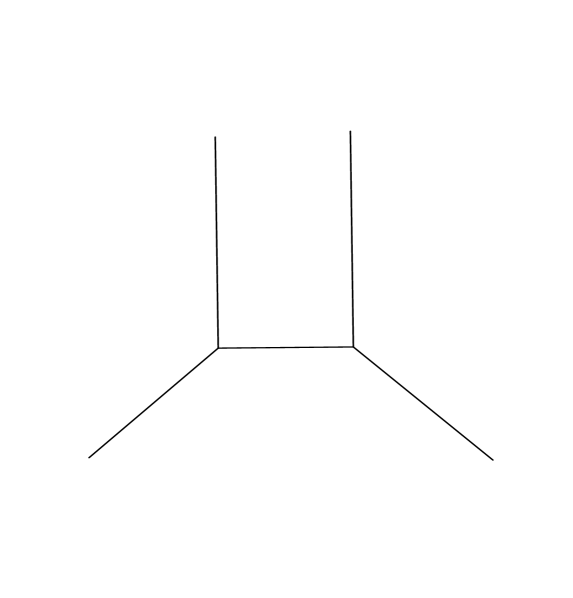
Here we consider a few simple examples of scattering amplitudes. The simplest type of 2-string scatterings corresponds to the following amplitude (see Figure 11):

$$(1,0)+(0,1)\rightarrow(1,0)+(0,1)$$

which can be viewed as the amplitude for

$${\cal A}=\langle\Phi((1,0),\theta_{1})\Phi((0,1),\theta_{2})\Phi((-1,0),\theta_{3})\Phi((0,-1),\theta_{4})\rangle$$

Using momentum conservation, and shifting two of the $\theta_{2}=\theta_{3}=0$, the amplitude will only depend on $\theta_{1}=\theta$. Dropping the delta function, we have the following answer of this scattering:

Figure 12: Another simple scattering amplitude with no internal loops.

$${\cal A}=\prod_{i,j,k,l=1}^{\infty}(1-q_{1}^{i}q_{2}^{j}\ e^{i\theta})(1-q_{1}^{k}q_{2}^{l}\ e^{-i\theta})$$

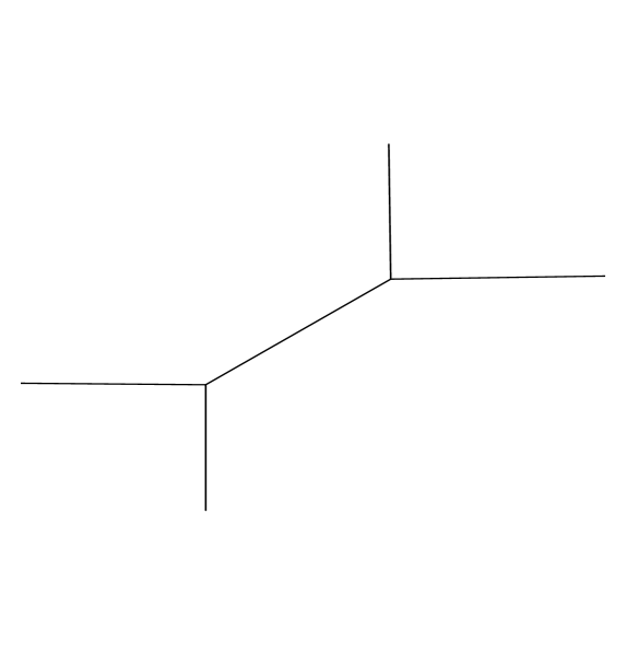
This corresponds to the $O(-1)+O(-1)$ geometry over ${\bf P}^{1}$ and has $g=0$. Another simple two particle $g=0$ scattering is (see Figure 12)

$$(1,0)+(1,0)\rightarrow(1,-1)+(1,1)$$

leading to the amplitude

$${\cal A}=\prod_{i,j,k,l=1}^{\infty}{1\over(1-q_{1}^{i}q_{2}^{j}\ e^{i\theta})(1-q_{1}^{k}q_{2}^{l}\ e^{-i\theta})}$$

Figure 13: The decay amplitude with one internal loop. The amplitude depends on no external momenta.

The higher genus amplitudes are more difficult to compute, though they can be computed. The simplest scattering corresponding to genus 1 corresponds to a three particle amplitude (see Figure 13):

$$(-2,1)\rightarrow(-1,2)+(-1,-1)$$

This scattering amplitude has no mass parameter $(N-3=3-3=0)$ so the amplitude depends only on $q_{1},q_{2}$. It corresponds to the superconformal index of M-theory on ${\bf C}^{3}/Z_{3}$. It can be computed using refined topological string (see iv ).

One can also compute amplitudes for non-toric geometries, for example corresponding to del Pezzo with 8 points blown up with $E_{8}$ global symmetry (corresponding to $SU(2)$ with 7 flavors sei ; dkv ; mseib . Using the result of tach this can be viewed as the result of the scattering of non-primitive winding modes:

$$(3,0)+(3,0)+(0,2)+(0,2)+(0,2)\rightarrow(1,1)+(1,1)+(1,1)+(1,1)+(1,1)+(1,1)$$

This has 8 parameters (11-3), and they can be identified with the Cartan of $E_{8}$ (or 7 masses of the fundamental $SU(2)$’s and one coupling constant of $SU(2)$) and has a genus $1$ worldsheet. This scattering amplitude has been recently computed using localization techniques for gauge theory amplitudes in kimyeong .

5 Open Questions

The primary question is to give a direct definition of the string theory we have provided evidence for. It is also natural to ask what is the relation of this string theory to $N=2$ string theory ov ?. The fact that both are defined in 4 dimensions with a complex structure suggests some relation between the two. In fact there are more common roots: They both seem to be related to integrable structures. Self-dual geometries and connections, which is the backbone of $N=2$ string theory is deeply rooted in integrable structures. On the other hand the worldsheet which underlies the scattering amplitude of the string we have proposed, is related to quantum version of Seiberg-Witten curve which again is deeply connected with integrable structures (see in particular nekshat ). Both the $N=2$ strings and the string being proposed here have effectively the same on-shell degrees of freedom corresponding to one scalar field in 4d. This is because choosing a winding vector has effectively two degrees of freedom (corresponding to integral points on ${\bf R}^{2}$) and in addition the momentum $\theta$, leading to three parameters to vary, just as one would expect for a massless scalar field in 4d which is the on shell degree of freedom of $N=2$ strings. It could be that to connect the two we need to introduce additional background branes in the $N=2$ string, as in the space-time filling coisotropic brane, making the space-time effectively non-commutative.

It is also clear that some aspects of the vertex for the string theory we have proposed need to be developed further. In particular currently we do not have a simple vertex which capture multiple winding strings. In particular as we have noted we need to develop techniques to compute an additional cubic and quartic type vertices. It would be important to extend the topological vertex formalism to this case. Also aspects of the refined topological string need to be better understood. In particular one needs to extend the non-commutative background to include both coupling constants in the refined case.

It is also natural to consider more general target space. For example it would be interesting to study this when $M={\bf C}^{2}$. This would correspond to SUSY amplitudes directly in 4d. Also it would to be interesting to consider $M$ being an arbitrary hyperKähler geometry. The fact that we can introduce 7-branes, already suggests that the elliptic fiber can vary (as the ${\bf T}^{2}$ is identified with the F-theory fiber), which is already a hyperKähler manifold which is not flat. Even though for the purposes of our paper we were able to push the 7-branes to infinity and treated the geometry as flat, this already shows that there is no inconsistency with having a non-flat hyperKähler geometry. Moreover the description in terms of $(B,A,A)$ branes in the background of cc branes supports this possibility, because these can be defined for arbitrary hyperKähler manifolds. Perhaps it would be natural to leave two directions non-compact to correspond to the time directions. Even this restriction would allow some interesting additional possibilities: For example what would this theory correspond to when $M$ is the non-commutative version of $T^{*}\Sigma$ where $\Sigma$ is an arbitrary Riemann surface? Note that this space does admit a complete $(2,2)$ signature hyperKähler metric ov , where the fiber directions correspond to time-like components of the metric.

It is also natural to ask if there is twistorial version of this theory. Namely, we have chosen a constant background B-field in 4-dimensional flat space. Different choices of such a $B$, where we can integrate over, can be viewed as a twistorial version of this theory.

The results presented here suggest that studying supersymmetric partition functions for a family of quantum theories in a given dimension may lead to a single unifying theory. In the 5d case, we found a string theory. I conjecture that this structure will also be true in other dimensions. It would be interesting to study this question and ask which unifying quantum theory, if any, underlies the supersymmetric partition functions for a family of quantum theories in a given dimension.

References

- (1) V. Pestun, “Localization of gauge theory on a four-sphere and supersymmetric Wilson loops,” Commun.Math.Phys. 313 (2012) 71–129, arXiv:0712.2824 [hep-th].
- (2) S. Cecotti and C. Vafa, “Topological antitopological fusion,” Nucl.Phys. B367 (1991) 359–461.
- (3) M. R. Douglas, S. H. Katz, and C. Vafa, “Small instantons, Del Pezzo surfaces and type I-prime theory,” Nucl.Phys. B497 (1997) 155–172, arXiv:hep-th/9609071 [hep-th].
- (4) D. R. Morrison and N. Seiberg, “Extremal transitions and five-dimensional supersymmetric field theories,” Nucl.Phys. B483 (1997) 229–247, arXiv:hep-th/9609070 [hep-th].
- (5) K. A. Intriligator, D. R. Morrison, and N. Seiberg, “Five-dimensional supersymmetric gauge theories and degenerations of Calabi-Yau spaces,” Nucl.Phys. B497 (1997) 56–100, arXiv:hep-th/9702198 [hep-th].
- (6) S. Katz, P. Mayr, and C. Vafa, “Mirror symmetry and exact solution of 4-D N=2 gauge theories: 1.,” Adv.Theor.Math.Phys. 1 (1998) 53–114, arXiv:hep-th/9706110 [hep-th].
- (7) N. C. Leung and C. Vafa, “Branes and toric geometry,” Adv.Theor.Math.Phys. 2 (1998) 91–118, arXiv:hep-th/9711013 [hep-th].
- (8) O. Aharony, A. Hanany, and B. Kol, “Webs of (p,q) five-branes, five-dimensional field theories and grid diagrams,” JHEP 9801 (1998) 002, arXiv:hep-th/9710116 [hep-th].
- (9) A. Iqbal and C. Vafa, “Work to appear,”.
- (10) M. Aganagic, A. Klemm, M. Marino, and C. Vafa, “The Topological vertex,” Commun.Math.Phys. 254 (2005) 425–478, arXiv:hep-th/0305132 [hep-th].
- (11) A. Iqbal, C. Kozcaz, and C. Vafa, “The refined topological vertex,” JHEP 10 (2009) 069, arXiv:hep-th/0701156.
- (12) H. Ooguri and C. Vafa, “Geometry of N=2 strings,” Nucl.Phys. B361 (1991) 469–518.
- (13) D. Gaiotto, “N=2 dualities,” JHEP 1208 (2012) 034, arXiv:0904.2715 [hep-th].
- (14) E. Witten, “Phase transitions in M theory and F theory,” Nucl.Phys. B471 (1996) 195–216, arXiv:hep-th/9603150 [hep-th].
- (15) F. Benini, S. Benvenuti, and Y. Tachikawa, “Webs of five-branes and N=2 superconformal field theories,” JHEP 0909 (2009) 052, arXiv:0906.0359 [hep-th].
- (16) M. Aganagic and C. Vafa, “Mirror symmetry, D-branes and counting holomorphic discs,” arXiv:hep-th/0012041 [hep-th].
- (17) M. Aganagic, A. Klemm, and C. Vafa, “Disk instantons, mirror symmetry and the duality web,” Z.Naturforsch. A57 (2002) 1–28, arXiv:hep-th/0105045 [hep-th].
- (18) S. Gukov and E. Witten, “Gauge Theory, Ramification, And The Geometric Langlands Program,” arXiv:hep-th/0612073 [hep-th].
- (19) C. Kozcaz, S. Pasquetti, and N. Wyllard, “A and B model approaches to surface operators and Toda theories,” JHEP 1008 (2010) 042, arXiv:1004.2025 [hep-th].
- (20) T. Dimofte, S. Gukov, and L. Hollands, “Vortex Counting and Lagrangian 3-manifolds,” Lett.Math.Phys. 98 (2011) 225–287, arXiv:1006.0977 [hep-th].
- (21) R. Dijkgraaf, C. Vafa, and E. Verlinde, “M-theory and a topological string duality,” arXiv:hep-th/0602087.
- (22) H. Awata and H. Kanno, “Refined BPS state counting from Nekrasov’s formula and Macdonald functions,” Int.J.Mod.Phys. A24 (2009) 2253–2306, arXiv:0805.0191 [hep-th].
- (23) R. Gopakumar and C. Vafa, “On the gauge theory/geometry correspondence,” Adv. Theor. Math. Phys. 3 (1999) 1415–1443, arXiv:hep-th/9811131.
- (24) N. Nekrasov and A. Okounkov, “Work to appear,”.
- (25) M. Aganagic and S. Shakirov, “Work to appear,”.
- (26) M. Aganagic, R. Dijkgraaf, A. Klemm, M. Marino, and C. Vafa, “Topological strings and integrable hierarchies,” Commun.Math.Phys. 261 (2006) 451–516, arXiv:hep-th/0312085 [hep-th].
- (27) R. Dijkgraaf, L. Hollands, P. Sulkowski, and C. Vafa, “Supersymmetric gauge theories, intersecting branes and free fermions,” JHEP 0802 (2008) 106, arXiv:0709.4446 [hep-th].
- (28) N. Seiberg and E. Witten, “String theory and noncommutative geometry,” JHEP 9909 (1999) 032, arXiv:hep-th/9908142 [hep-th].
- (29) A. Kapustin and E. Witten, “Electric-Magnetic Duality And The Geometric Langlands Program,” Commun.Num.Theor.Phys. 1 (2007) 1–236, arXiv:hep-th/0604151 [hep-th].
- (30) A. Kapustin and D. Orlov, “Remarks on A branes, mirror symmetry, and the Fukaya category,” J.Geom.Phys. 48 (2003) 84, arXiv:hep-th/0109098 [hep-th].
- (31) H.-C. Kim, S.-S. Kim, and K. Lee, “5-dim Superconformal Index with Enhanced En Global Symmetry,” arXiv:1206.6781 [hep-th].
- (32) D.-E. Diaconescu, B. Florea, and N. Saulina, “A Vertex formalism for local ruled surfaces,” Commun.Math.Phys. 265 (2006) 201–226, arXiv:hep-th/0505192 [hep-th].
- (33) A. Hanany and E. Witten, “Type IIB superstrings, BPS monopoles, and three-dimensional gauge dynamics,” Nucl.Phys. B492 (1997) 152–190, arXiv:hep-th/9611230 [hep-th].
- (34) D.-E. Diaconescu, A. Iqbal, and C. Vafa, “Work in progress,”.
- (35) R. Dijkgraaf and C. Vafa, “Toda Theories, Matrix Models, Topological Strings, and N=2 Gauge Systems,” arXiv:0909.2453 [hep-th].
- (36) M. C. Cheng, R. Dijkgraaf, and C. Vafa, “Non-Perturbative Topological Strings And Conformal Blocks,” JHEP 1109 (2011) 022, arXiv:1010.4573 [hep-th].
- (37) T. J. Hollowood, A. Iqbal, and C. Vafa, “Matrix models, geometric engineering and elliptic genera,” JHEP 0803 (2008) 069, arXiv:hep-th/0310272 [hep-th].
- (38) R. Dijkgraaf, E. P. Verlinde, and H. L. Verlinde, “Matrix string theory,” Nucl.Phys. B500 (1997) 43–61, arXiv:hep-th/9703030 [hep-th].
- (39) L. F. Alday, D. Gaiotto, and Y. Tachikawa, “Liouville Correlation Functions from Four-dimensional Gauge Theories,” Lett.Math.Phys. 91 (2010) 167–197, arXiv:0906.3219 [hep-th].
- (40) N. Wyllard, “A(N-1) conformal Toda field theory correlation functions from conformal N = 2 SU(N) quiver gauge theories,” JHEP 0911 (2009) 002, arXiv:0907.2189 [hep-th].
- (41) D. Harlow, J. Maltz, and E. Witten, “Analytic Continuation of Liouville Theory,” JHEP 1112 (2011) 071, arXiv:1108.4417 [hep-th].
- (42) N. Seiberg, “Five-dimensional SUSY field theories, nontrivial fixed points and string dynamics,” Phys.Lett. B388 (1996) 753–760, arXiv:hep-th/9608111 [hep-th].
- (43) N. Berkovits and C. Vafa, “N=4 topological strings,” Nucl.Phys. B433 (1995) 123–180, arXiv:hep-th/9407190 [hep-th].
- (44) H. Ooguri and C. Vafa, “All loop N=2 string amplitudes,” Nucl.Phys. B451 (1995) 121–161, arXiv:hep-th/9505183 [hep-th].
- (45) N. A. Nekrasov and S. L. Shatashvili, “Supersymmetric vacua and Bethe ansatz,” Nucl. Phys. Proc. Suppl. 192-193 (2009) 91–112, arXiv:0901.4744 [hep-th].
- (46) J. Heckman, “Talk given in Strings 2012, based on joint work with H. Verlinde,”.