Occupation of X-ray selected galaxy groups by X-ray AGN

Abstract

We present the first direct measurement of the mean Halo Occupation Distribution (HOD) of X-ray selected AGN in the COSMOS field at $z\leq 1$, based on the association of 41 XMM and 17 C-COSMOS AGN with member galaxies of 189 X-ray detected galaxy groups from XMM and Chandra data.We model the mean AGN occupation in the halo mass range $logM_{200}[M_{\odot}]=13-14.5$ with a rolling-off power-law with the best fit index $\alpha=0.06(-0.22;0.36)$ and normalization parameter $f_{a}=0.05(0.04;0.06)$. We find the mean HOD of AGN among central galaxies to be modelled by a softened step function at log$M_{h}>$log$M_{min}=12.75(12.10,12.95)$$M_{\odot}$ while for the satellite AGN HOD we find a preference for an increasing AGN fraction with $M_{h}$ suggesting that the average number of AGN in satellite galaxies grows slower ($\alpha_{s}<0.6$) than the linear proportion ($\alpha_{s}=1$) observed for the satellite HOD of samples of galaxies. We present an estimate of the projected auto correlation function (ACF) of galaxy groups over the range of $r_{p}=$ 0.1 - 40 h^-1Mpc at $\langle z\rangle=0.5$. We use the large-scale clustering signal to verify the agreement between the group bias estimated by using the observed galaxy groups ACF and the value derived from the group mass estimates. We perform a measurement of the projected AGN-galaxy group cross-correlation function, excluding from the analysis AGN that are within galaxy groups and we model the 2-halo term of the clustering signal with the mean AGN HOD based on our results.

1. Introduction

In the past decade it has become clear that the majority of galaxies have likely had one or more brief active periods, shifting our view of astrophysical black holes (BHs) from the role of exotic phenomena to fundamental ingredients of cosmic structures. The question of when and under which physical conditions the active galactic nuclei (AGN) activate is important for understanding not only the origin and evolution of BHs but also the origin and evolution of galaxies.

The clustering analysis can powerfully test theoretical model predictions and address which physical processes trigger AGN activity. In the framework of the cold dark matter structure formation (CDM), the spatial distribution of AGN in the Universe (described by the correlation function, CF) can be related to how AGN are biased with respect to the underlying matter distribution and to the typical mass of dark matter halos (DMHs) in which they reside. There have been several studies of the bias evolution of optical quasars with redshift, based on survey such as 2QZ and SDSS (Croom et al., 2005; Porciani & Norberg, 2006; Shen et al., 2009; Ross et al., 2009). All the previous studies infer the picture that the quasar bias evolves with redshift following a constant mass evolution in the range log$M_{h}$[h${}^{-1}M_{\odot}$] $\sim 12.5-13$, i.e. halo masses similar to group scales, where the combination of low velocity dispersion and moderate galaxy space density yields to the highest probability of a close encounter (Hopkins et al., 2008; McIntosh et al., 2009). Models of major mergers between gas-rich galaxies appear to naturally produce many observed properties of quasars, such as the shape and the evolution of the quasar luminosity function and the large-scale quasar clustering as a function of luminosity and redshift (Hopkins et al., 2007, 2008; Shen, 2009; Shankar et al., 2009, 2010; Bonoli et al., 2009), supporting the scenario in which major mergers dominate the bright quasar populations. On the other hand, the majority of the results on the clustering of X-ray selected AGN, suggest a picture where moderate-luminosity AGN live in massive DMHs ($12.5<logM_{h}$[h${}^{-1}M_{\odot}$] $<13.5$) up to $z\sim 2$ (Gilli et al., 2005; Yang et al., 2006; Gilli et al., 2009; Hickox et al., 2009; Coil et al., 2009; Krumpe et al., 2010; Cappelluti et al., 2010; Krumpe et al., 2010; Allevato et al., 2011; Miyaji et al., 2011), i.e. X-ray selected AGN samples appear to cluster more strongly than luminous quasars (see Cappelluti, Allevato & Finoguenov, 2012, for a review on the argument). The reason for this is not completely clear, but several studies argued that this large bias and DMH masses could suggest a different AGN triggering mechanism with respect to bright quasars characterized by galaxy merger-induced fueling. Several studies on the morphology of the AGN host galaxies have demonstrated that major mergers of galaxies are not likely to be the single dominant mechanism responsible for triggering AGN activity at low ($z\sim 1$) (Georgakakis et al., 2007; Silverman et al., 2009; Georgakakis et al., 2009; Dunlop et al., 2003; Grogin et al., 2005; Pierce et al., 2007; Gabor et al., 2009; Reichard et al., 2009; Tal et al., 2009; Cisternas et al., 2011; Silverman et al., 2011) and high redshift ($z\sim$ 2) (Rosario et al., 2011; Kocevski et al., 2011; Schawinski et al., 2011).

The theoretical understanding of galaxy clustering and bias factor has been greatly enhanced through the Halo Occupation Distribution (HOD) framework. In this framework, the virialised DMH with typical overdensities of $\Delta_{200}$ (defined w.r.t. the mean density) are described in terms of the probability $P(N|M)$ of a halo of given mass $M$ of having $N$ galaxies. A simple way to model the complicated shape of $N(M)$ is by assuming the existence of two separate galaxy populations within halos, central and satellite galaxies. This method has been used extensively to interpret galaxy CFs (Hamana et al., 2004; Tinker et al., 2005; Phleps et al., 2006; Zheng et al., 2007; Zehavi et al., 2010; Zheng et al., 2009) to constrain how various galaxy samples are distributed among DMH as well as whether these galaxies occupy the centers of the DMHs or are satellite galaxies (Kravtsov et al., 2004; Zheng et al., 2005; Zehavi et al., 2005; Richardson et al., 2012). These two populations can be modeled with an HOD described by a step function above a halo mass limit for central galaxies, and a power-law for satellite galaxies.

Similarly, the problem of discussing the abundance and spatial distribution of AGN can be reduced to studying how they populate their host halos. In fact the observed departure of the AGN CF from a power law on small scales (1-2 h^-1Mpc) can be physically interpreted in the language of the halo model, as the transition between two scales - from small scales lying within the DMHs (1-halo term) to those larger than the halo (2-halo term). The 1-halo term constrains the HOD of satellite AGN and gives us the average profile of pairs of AGN in groups and clusters of galaxies. The 2-halo term reflects the large-scale AGN bias driven by the typical mass of the hosting halos.

Due to the low number density of AGN, there have been few results in the literature studying the AGN correlation function using HOD modeling. Previous works of Padmanabhan et al. (2009) at $z<0.6$ and Shen et al. (2010) at $z=3-4$ on QSO using the HOD modeling found that $>$25% and $\geqslant$10% of their QSOs, respectively, are satellites. Miyaji et al. (2011) described for the first time the shape of the HOD of X-ray selected AGN. By using the cross correlation function of ROSAT-RASS AGN with SDSS galaxies, they modelled the mean AGN occupation of DMHs suggesting that the satellite AGN fraction increases slow (or may even decrease) with $M_{h}$, in contrast with the satellite HOD of luminosity-limited samples of galaxies. Cosmological hydrodynamic simulations have been performed in Chatterjee et al. (2012) to study the mean occupation function of low-luminosity AGN as function of redshift and luminosity. They used a softened step function for the central component plus a rolling-off power-law for the satellite component with $\alpha=0.3-1.4$ depending on the redshift and AGN luminosity. Their results suggest a strong evolution of the AGN occupancy in the redshift range $z=1-3$ estimated at three different luminosities $L_{BOL}\geq 10^{38},10^{40},10^{42}$ s^-1erg. Richardson et al. (2012) modelled the HOD of SDSS quasars at $z\sim 1.4$ following this parametrization. They found that the satellite occupation becomes significant at mass $\sim 10^{14}$h${}^{-1}M_{\odot}$, i.e. only the most massive halos host multiple quasars at this redshift and only a small satellite fraction ($f_{sat}=7.4\pm 1.3\times 10^{-4}$) of SDSS quasars is required to fit the clustering signal at small scales. Moreover, they measured that the quasars HOD steepens considerably going from z=1.4 to 3.2 over halo mass scales $10^{13-14}$ h${}^{-1}M_{\odot}$ and that the characteristic halo mass increases with z for central quasars.

Despite the diverse methods for studying the HOD, counting the number of AGN within galaxy groups can constrain quite directly the average AGN number within a halo as a function of halo mass. The total mass of galaxy groups can be estimated via gravitational lensing and the distribution of AGN within halos can be investigated in groups by means of the distribution of the AGN host galaxies. Separating the contribution to the occupation of halos from AGN in satellite or central galaxies can advance our understanding of the co-evolution AGN/galaxy and is related to the mechanism of AGN activation.

On the other hand, the cross-correlation (CCF) of AGN with galaxy groups provides additional information about how galaxies and BH co-evolve in dense environments. In fact the physical processes that drive galaxy evolution, such as the available cold gas to fuel star formation and the BH growth, are substantially different in groups and clusters compared to the field. Many studies over the past decade have presented an evidence that AGN at $z\sim 1$ are more frequently found in groups compared to galaxies (Georgakakis et al. 2008, Arnold et al. 2009). X-ray observations reveal that a significant fraction of high-z clusters show overdensities of AGNs in their outskirts (Henry et al. 1991, Cappi et al. 2001, Ruderman et al. 2005, Cappelluti et al. 2005).

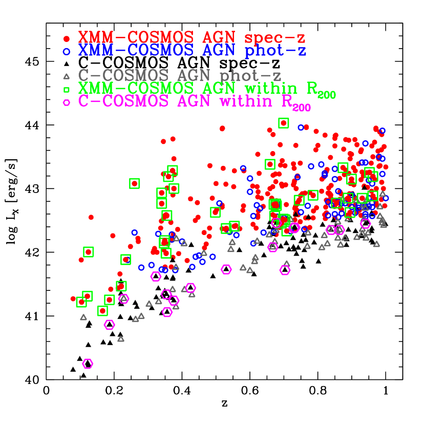
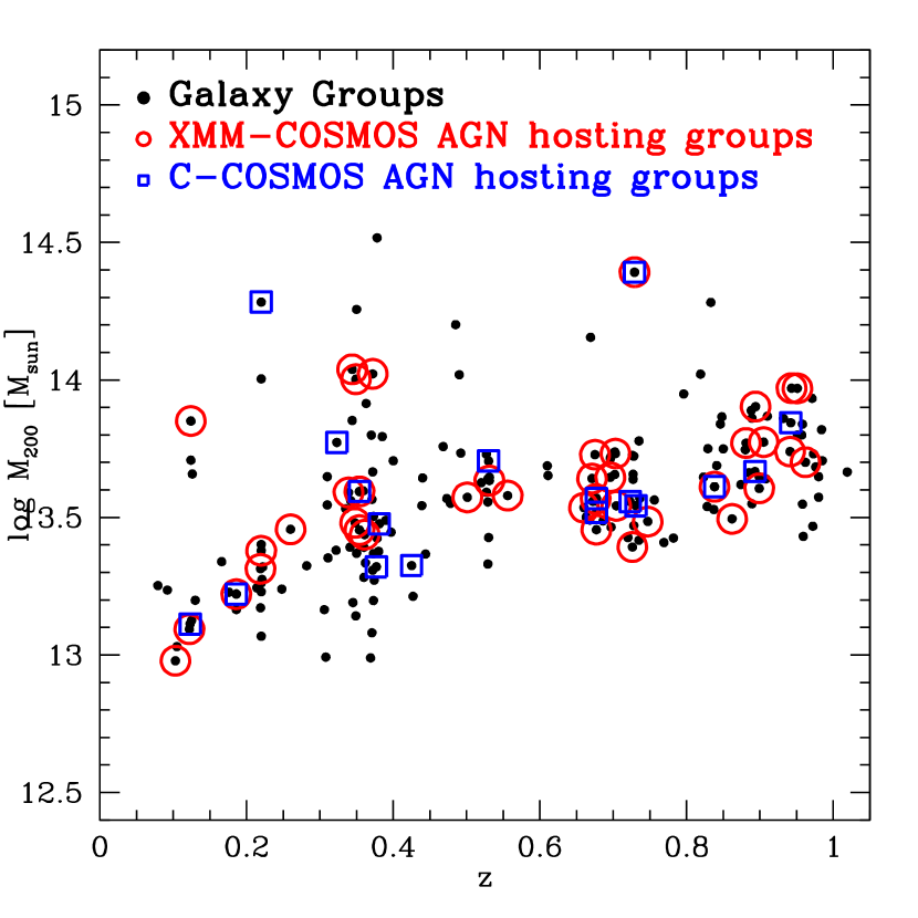
Figure 1.— Left panel: X-ray rest-frame soft luminosity $L_{X}$ as a function of redshift for XMM-AGN (circles) and C-COSMOS selected AGN (triangle) with know spec-z (filled) and or phot-z (open). The open green squares indicate XMM-AGN within galaxy groups, while the open magenta hexagons represent 17 additional C-COSMOS slected AGN in galaxy groups. Right panel: Galaxy group masses $M_{200}$ as a function of redshift for the whole galaxy group sample (black circles) while open circles (squares) indicate XMM-AGN (C-COSMOS AGN) hosting groups. The mass estimates are defined with respect to 200 times the mean density, in units of $M_{\odot}$.

In this paper, we perform the first direct measurement of the mean halo occupation of X-ray AGN and of the projected cross-correlation function of AGN with galaxy groups, using a sample of X-ray selected AGN and galaxy groups in the COSMOS field at $z\leq 1$, from XMM and Chandra data. We use a $\Lambda$CDM cosmology with $\Omega_{M}=0.28$, $\Omega_{\Lambda}=0.72$, $\Omega_{b}=0.045$, $\sigma_{8}=0.8$. For comparison with previous measurements we refer to correlation lengths and distances in units of $h^{-1}$ Mpc comoving, where $H_{0}=100$ h km s^-1 Mpc^-1. AGN luminosities and galaxy groups masses are calculated using $h$ = 0.72.

2. The Catalogs

2.1. AGN Catalog

The Cosmic Evolution Survey (COSMOS) is a multiwavelength survey over $1.4\times 1.4$ deg² of equatorial sky observed by the most advanced astronomical facilities HST (Scoville et al., 2007), SUBARU (Taniguchi et al., 2007), Spitzer (Sanders et al., 2007), GALEX (Zamojski et al., 2007), XMM-Newton (Hasinger et al., 2007; Cappelluti et al., 2007, 2009), Chandra (Elvis et al., 2009; Puccetti et al., 2009), designed to thoroughly probe the evolution of galaxies, AGN, and dark matter in the context of their cosmic environment (LSS). XMM-Newton surveyed $2.13$ deg² of this field in the 0.5-10 keV energy band for a total of $\sim$ 1.55 Ms providing a large sample of 1822 point-like X-ray sources (Cappelluti et al., 2009), down to limiting fluxes of $\sim 5\times 10^{-16}$, $\sim 3\times 10^{-15}$ and $\sim 7\times 10^{-15}$ erg cm^-2s^-1 in the soft, hard and ultra hard band, respectively.

The inner part of the COSMOS field ($\sim 0.92$ deg²) has been imaged for a total of 1.8 Ms by Chandra down to limiting fluxes 3-4 times deeper than XMM-COSMOS. Of the 1822 XMM sources, 945 have been observed by Chandra and 875 of them are presented in the C-COSMOS point-like source catalog (Elvis et al., 2009; Puccetti et al., 2009; Civano et al., 2012). Brusa et al. (2010) presented the XMM-COSMOS multiwavelength catalog of X-ray sources with optical/near-infrared identification, multiwavelength properties and redshift information. Starting from this catalog, we restricted the analysis to a sample of X-ray AGN (we removed normal galaxies and ambiguous sources) detected in the soft band which guarantees the largest sample of X-ray AGN in the COSMOS field, compared to AGN observed in the hard or ultra-hard band. Moreover, the selection in only one band allows a more simple treatment of the AGN X-ray luminosity function used to correct the AGN HOD (§3) and of the XMM-and C-COSMOS sensitivity maps used to generate the AGN random catalog (§4.3).

Specifically, we selected a sample of 280 and 83 soft XMM-COSMOS AGN with spectroscopic and photometric redshift (Salvato et al., 2011) $z\leq 1$, respectively. The use of photometric redshifts for group membership assignment has been successfully demonstrated in George et al. (2011). Note that 184/363 sources are also Chandra detected AGN. In order to test if the AGN halo occupation significantly changes including sources from the C-COSMOS catalog that are only Chandra detected (hereafter C-COSMOS AGN) (see §3), we included in the analysis a sample of 107 and 61 AGN, detected in the soft band, with known spectroscopic or photometric redshifts $z\leq 1$, respectively. The rest-frame soft X-ray luminosity as a function of redshift is shown in Fig. 1 (Left Panel) for XMM-COSMOS AGN (circles) and C-COSMOS AGN (triangles).

2.2. Galaxy Group Catalog

We used a catalog with 270 galaxy groups, detected in the co-added XMM-Newton and Chandra data. The general data reduction process is described in Finoguenov et al. (2007) and details regarding improvements and modification to the initial catalog are given in Leauthaud et al. (2010) and George et al. (2011). The identification of the groups has been done using the red sequence technique, and spectroscopic identification of groups has been achieved through zCOSMOS-BRIGHT program (Lilly et al., 2009), targeted follow-up using IMACS/Magellan and FORS2/VLT (George et al., 2011), Gemini GMOS-S (Balogh et al., 2011) as well as through secondary targets on Keck runs by COSMOS collaboration. At $z\leq 1$ the spectroscopic completeness has achieved 90% (A. Finoguenov 2012, in preparation).

As described in Leauthaud et al. (2010), the total X-ray fluxes have been obtained from the measured fluxes by assuming a beta profile and by removing the flux that is due to embedded AGN point sources. Some of the faint Chandra AGN could not be removed from the group fluxes, with their contribution to the total flux being $<10\%$. The rest-frame luminosities have been computed in Finoguenov et al. (2007) and Leauthaud et al. (2010) from the total flux following $L_{0.1-2.4keV}=4\pi d_{L}^{2}K(z,T)C_{\beta}(z,T)F_{d}$, where $K(z,T)$ is the K-correction and $C_{\beta}(z,T)$ is an iterative correction factor, while to estimate the temperature of each group they used the $L_{X}-T$ relation of Markevitch (1998).

A quality flag (hereafter ’XFLAG’) is assigned to the reliability of the optical counterpart, with flags 1 and 2 indicating a secure association, and higher flags indicating potential problems due to projections with other sources or bad photometry due to bright stars in the foreground. In detail, XFLAG=1,2 are assigned to groups with a confident spectroscopic association, while systems with only the red sequence identification have XFLAG=3 (see Leauthaud et al., 2010, for more details).

The line-of-sight position of the group is assigned to be the centroid of the X-ray emission (the accuracy of the determination of the X-ray center is higher for XFLAG=1). If the X-ray centroid is not precise enough to be used directly,the Most Massive Central Galaxy (MMCG) located near the peak of the X-ray emission has been used to trace the center of the DM halos of groups (see Leauthaud et al., 2010; George et al., 2011, for more details). Group masses $M_{200}$ are assigned from an empirical mass-luminosity relation, described in Leauthaud et al. (2010),

$$log_{10}(M_{200,c})=p_{0}-log_{10}E(z)+log_{10}(M_{0})$$ (1)

$$+p_{1}[log_{10}(L_{x}/E(z))-log_{10}(L_{0})]$$

where $M_{200}$ is the mass within the radius containing the density of matter 200 times the critical density, in units of $M_{\odot}$. $\left\{p_{0},p_{1}\right\}=\left\{0.729538,0.561657\right\}$ are the fitting parameters, $\left\{logM_{0},logL_{0}\right\}=\left\{13,42.5\right\}$ are the calibration parameters and $E(z)$ is the correction for redshift evolution of scaling relations, which has been shown in Leauthaud et al. (2010) to reproduce well the $L_{X}-M$ relation of COSMOS groups.

In order to be consistent in comparing these mass values with the ones obtained studying the clustering properties of groups, we accounted for the difference between the mass defined with respect to 200 times the critical density and with respect to 200 times the mean density (hereafter $M_{200}$ refers to masses obtained using the definition with respect to the mean density). In fact, the absolute bias which we are going to derive from the DM correlation function is based on the shape of the DM mass function defined with respect to the mean density. Starting from the Navarro-Frenk-White (NFW) profile with a concentration parameter $c=5$, we derived the relation between the two mass definitions, $M_{200,m}=M_{200,c}\times\Omega(z)^{-0.134}$.

In this work, we make use of galaxy groups with $z\leq 1$ and identification flag $XFLAG\leq 3$ which removes problematic identification cases, obtaining a catalog of 189 X-ray galaxy groups over 1.64 deg² with a rest-frame 0.1-2.4 keV luminosity range of $41.3<log(L_{X}[s^{-1}$erg]$)<44.1$, and mass range of $13<logM_{200}[M_{\odot}]<14.5$ (see Fig. 1, Right Panel).

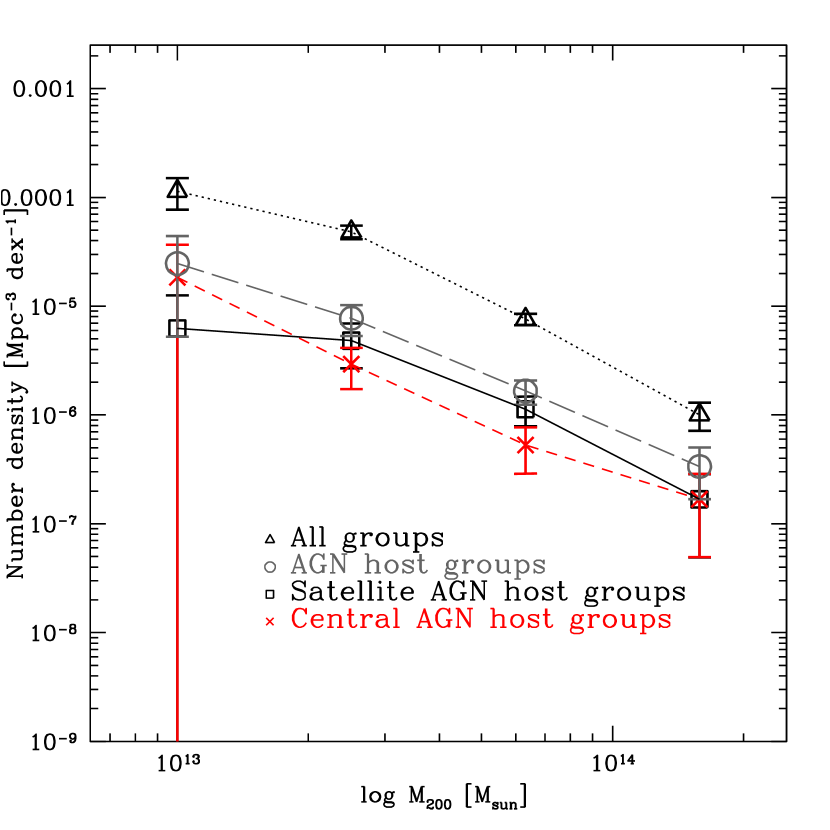
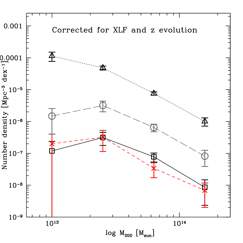
Figure 2.— Left Panel: Mass function of X-ray galaxy groups (triangles) and AGN host groups (circles). The black squares (red crosses) show the mass function of groups hosting an AGN in satellite (central) galaxies. Right Panel: Same as left panel when correcting for the AGN soft XLF and the redshift evolution.

2.3. AGN in galaxy groups

We define group members as AGN located within $<3\sigma$ and $<R_{200}$ from the group centers, where $\sigma$ is the group line-of-sight velocity dispersion and $R_{200}$ is the virial radius of a group within which the mean density is 200 times the mean density of the Universe at the group redshift.

In this analysis we used the sample of 363 XMM-COSMOS AGN with $z\leq 1$ described in §2.1 and we found 41 sources (35/41 are also Chandra detected) in galaxy groups with median $\langle z\rangle=0.55$ and median $\langle L_{X}\rangle=10^{42.6}$ $s^{-1}$erg. When we include in the analysis the sample of 168 C-COSMOS AGN (§2.1), we found 17 additional AGN in galaxy groups, with known spectroscopic or photometric $z\leq 1$. As expected C-COSMOS AGN have lower soft fluxes respect to XMM-COSMOS AGN at any redshift, with a median $L_{X}=10^{41.7}$ $s^{-1}$erg. In particular we found 2 galaxy groups at $z\sim 0.1$ and 2 groups at $z\sim 0.7-0.8$ with 2 AGN per halo and 1 group with 3 AGN at $z\sim 0.35$. All the properties of AGN and galaxy group samples are summarized in Table 1, while Table 2 shows the catalog of 58 XMM + C-COSMOS AGN in galaxy groups. For the sources with known spectroscopic redshifts (47/58) we know the classification in BL or non-BL AGN as described in Brusa et al. (2010) and Civano et al. (2012) for XMM and C-COSMOS AGN, respectively. In detail, we found 43 non-BL and 4 BL in the XMM + C-COSMOS AGN sample. Fig. 1 (Left Panel) shows the rest-frame soft X-ray luminosity as a function of redshift for the subsamples of XMM (green squares) and C-COSMOS selected AGN (magenta hexagon) within $R_{200}$.

We cross-matched the sample of AGN in groups with a galaxy membership catalog (Leauthaud et al., 2007; George et al., 2011) and we verified that AGN classified as group members based on our method, have host galaxies associated with the same galaxy groups. We divided the sample of 58 AGN in groups in two subsets, according to their association with BCGs. In detail we found that 22/58 (16/41) AGN are in central galaxies, while 36/58 (25/41) are in satellites.

Table 1Properties of the Group and AGN Samples

(1)	(2)	(3)	(4)
Sample	N	$\langle z\rangle$	$\langle L_{X}\rangle$
XMM-AGN	363	0.66	$10^{42.8}$
C-COSMOS AGN	168	0.56	$10^{41.8}$
XMM-AGN in $R_{200}$	41	0.55	$10^{42.6}$
C-COSMOS AGN in $R_{200}$	17	0.53	$10^{41.7}$
XMM-AGN in the field	253	0.67	$10^{42.8}$
XMM+C-COSMOS AGN in $R_{200}$	58	0.55	$10^{42.3}$
- Satellites	36	0.56	$10^{42.2}$
- Centrals	22	0.50	$10^{42.4}$
			$\langle M_{200}\rangle$
Galaxy Groups	189	0.56	$10^{13.60}$
XMM+C-COSMOS AGN host groups	52	0.55	$10^{13.62}$

3. Halo Mass Function and AGN HOD

Fig. 2 (Left Panel) shows the mass function of all X-ray galaxy groups and those marked by AGN presence, showing separately the contributions of groups hosting an AGN in central or satellite galaxies. We calculated the mass function by using the standard $1/V_{max}$ method (Schmidt 1968) and we counted twice galaxy groups with 2 AGN. Hence, in the $i^{th}$ mass bin, the comoving space density ($n_{i}$) and its corresponding error ($\sigma_{i}$) are computed by (see Bondi et al. 2008):

$$n_{i}=\sum_{j}\frac{1}{V_{max}^{j}} \sigma_{i}=\sum_{j}\sqrt{\left(\frac{1}{V_{max}^{j}}\right)^{2}}$$ (2)

In estimating the average number of AGN occupying a halo of mass $M_{200}$, some major effects need to be taken into consideration. The sample of AGN in $R_{200}$ is a flux-limited sample and brighter AGN are detected at higher redshift. Similarly, we observe galaxy groups with small halo mass only at low redshift. However the relatively small number of COSMOS AGN in galaxy groups does not allow us to select a volume complete subsample by using a cut in luminosity at log$L_{X}$[erg s^-1]=42.4. We have therefore made a correction for the effect of changes in the AGN density as a function of redshift and limiting luminosity, by using the AGN X-ray luminosity function (XLF). It has been shown in different works that the Luminosity Dependent Density Evolution (LDDE) model for the XLF provides the best framework that describes the evolutionary properties of AGN, both in the soft (Miyaji et al., 2000; Hasinger et al., 2005) and hard X-rays (Ueda et al., 2003; La Franca et al., 2005). In this paper we modelled the AGN soft XLF with the LDDE XLF described in Ebrero et al. (2009), because they modelled the soft XLF including in the analysis both type 1 and type 2 AGN, but we verified that using different best-fit parameters of the global XLF expression, the resulting mean AGN occupation stays within the error bars.

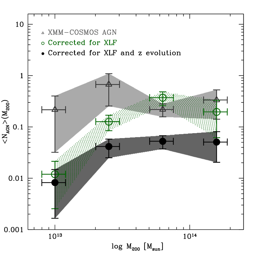
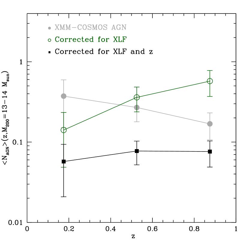
Figure 3.— Left Panel: Observed occupation of galaxy groups by XMM-COSMOS AGN as a function of the halo mass (open grey triangles) and after correcting for the soft XLF (green open circles) and for both the XLF and the AGN redshift evolution. Right Panel: Mean AGN occupation as a function of redshift for AGN hosting groups with $M_{200}=13-14M_{\odot}$ (colors with same meaning as left panel.)

Then for each AGN redshift we defined two weights: $w$ to correct for the fact that we are including in the analysis AGN with log$L_{X}$[erg s^-1]$<$42.2 and $w_{0}$ to correct for this effect plus the redshift evolution of the AGN density:

$$w(z)=\frac{\int_{42.4}^{\infty}\phi(z,L_{X})dL_{X}}{\int_{L_{lim}(z)}^{\infty}\phi(z,L_{X})dL_{X}}$$ (3)

$$w_{0}(z)=\frac{\int_{42.4}^{\infty}\phi(z=0,L_{X})dL_{X}}{\int_{L_{lim}(z)}^{\infty}\phi(z,L_{X})dL_{X}}$$ (4)

$\phi(z,L_{X})$ is the soft XLF proposed in Ebrero et al. (2009) and $L_{lim}$ depends on the survey flux limit and is a function of redshift. In detail, following Equations 9,11 and 12 and Table 2 in Ebrero et al. (2009), we described the shape of the present-day luminosity function with slopes $\gamma_{1}=0.72\pm 0.02$ and $\gamma_{2}=2.04\pm 0.04$, log$L_{0}$[h₇₀erg s^-1] = 43.65 $\pm$ 0.05 which is the value of the luminosity where the change of slope occurs and normalization $A=3.76\pm 0.38\times 10^{-6}$h${}_{70}^{3}$Mpc^-3. We estimated the evolution factor assuming $p_{1}=3.38\pm 0.09$, $p_{2}=-1.5$, $z_{c}=1.42$, log$L_{a}$ = 44.6h₇₀erg s^-1 and $\alpha=0.100\pm 0.005$.

Based on Eq. 3 and 4, the comoving space density $n_{i}$ of AGN hosting groups corrected for the XLF is given by:

$$n_{i}=\sum_{j}\frac{w^{j}(z,L_{X})}{V_{max,j}}$$ (5)

while the $n_{i}$ corrected for both the XLF and the z evolution is estimated by using:

$$n_{i}=\sum_{j}\frac{w_{0}^{j}(z=0,L_{X})}{V_{max,j}}$$ (6)

Fig. 2 (Right Panel) shows the mass function when all these effects are corrected.

The ratio between the mass function of X-ray groups hosting AGN within $R_{200}$ by that of all X-ray galaxy groups generates the mean AGN HOD, which describes the occupation of DM halos by AGN. Fig. 3 (Left Panel) shows the observed average number of XMM-COSMOS AGN in a halo of given mass as a function of $M_{200}$ (grey triangles) and the average number after correcting for the XLF (green open circles) and for both the XLF and the z evolution (black filled circles). The redshift evolution of the AGN fraction is shown in Fig. 2 (Right Panel). The grey circles represent the mean AGN occupation as a function of redshift for halos with $M_{200}=13-14M_{\odot}$ while the green circles and the black squares show the AGN fraction when we correct for the XLF only and for both the XLF and the z evolution effects, respectively. When we correct for the XLF, the mean occupation increases with z since in the AGN luminosity range of our interest, the AGN density increases with z, while the redshift correction removes this trend producing a constant AGN fraction.

We fitted the total AGN HOD assuming the model with a rolling-off power-law:

$$\langle N_{AGN}\rangle(M_{h})=f_{a}\left(\frac{M_{h}}{M_{1}}\right)^{\alpha}exp\left(\frac{M_{cut}}{M_{h}}\right)$$ (7)

where $f_{a}$ is the normalization, $M_{1}$ is the halo mass at which the number of central AGN is equal to that of satellite AGN, $M_{cut}$ is a cut-off mass scale. With our data alone, we cannot make meaningful constraints on $M_{1}$, therefore we fixed log$M_{1}=13.8M_{\odot}$ following the results of Miyaji et al. (2011). We verified that the result does not change for log$M_{1}=13-14.2M_{\odot}$, due to the fact that the fraction of AGN among central and satellite galaxies are comparable in this mass range. For the modelling of the rolling-off power-law, we assumed log$M_{cut}=13.4M_{\odot}$ which corresponds to the mass below which our data points decay exponentially.

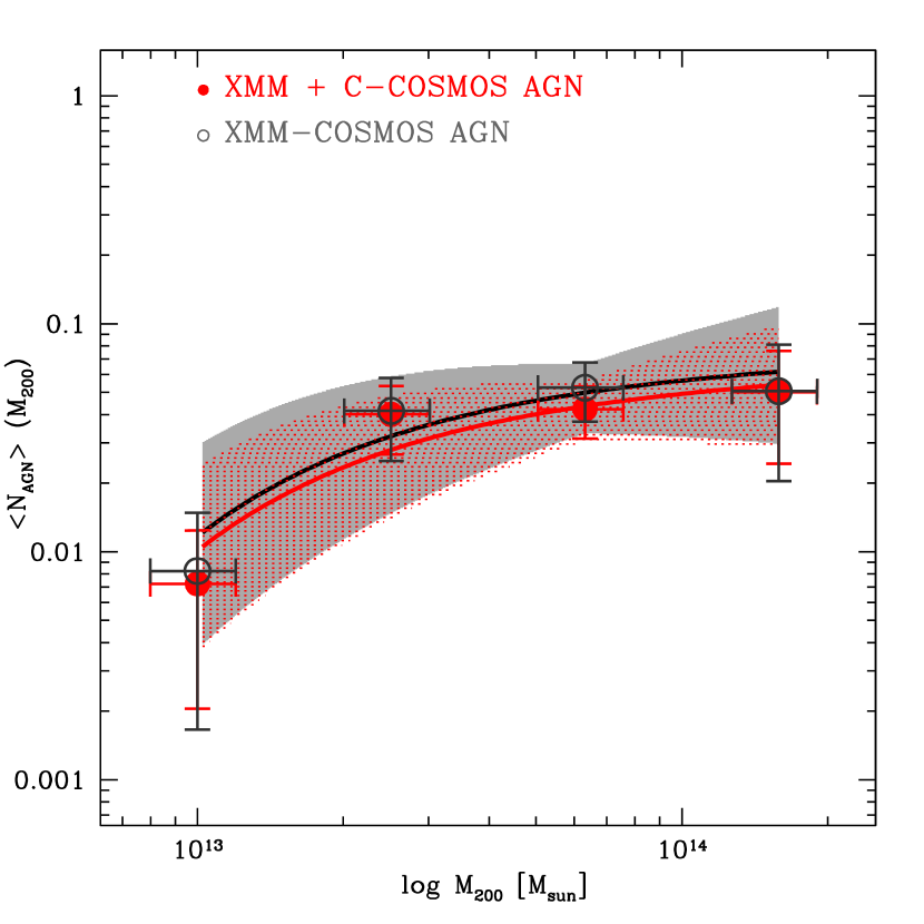
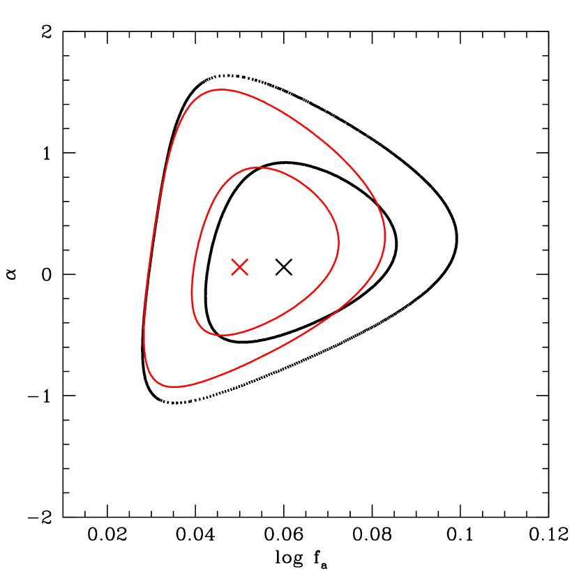
Figure 4.— Left Panel: Occupation of galaxy groups by 41 XMM-COSMOS AGN (black open circles) and 58 XMM + C-COSMOS AGN (red filled circles) as a function of the halo mass, when correcting for the XLF and for the redshift evolution of the AGN density. The fit assuming a rolling-off power-law dependence of the HOD is shown as the solid black lines (best fit) and shaded regions ($1\sigma$ confidence interval, $\Delta\chi^{2}=2.3$). Right Panel: the confidence contours of the power-law best-fit parameters $\alpha$ and $f_{a}$, for XMM-COSMOS AGN (black) and for XMM + C-COSMOS AGN (red) in galaxy groups. The contours mark the 68.3% and 95.4% confidence levels (respectively corresponding to $\Delta\chi^{2}$ = 2.3 and 6.17).

We obtained constraints in the ($\alpha$, $f_{a}$) - space and we found as best fit parameters of the mean AGN HOD, $\alpha=0.06(-0.22;+0.45)$ and $f_{a}=0.06(0.04;0.08)$, where the $68\%$ confidence interval for a combined two parameter fit ($\Delta\chi^{2}=2.3$) is given in the brackets. Fig. 4 (Left Panel) shows the mean occupation of XMM-COSMOS AGN with the best fit parameters (solid black line), and 1$\sigma$ confidence interval (shaded grey region), compared to the mean AGN HOD including C-COSMOS AGN in the analysis. The solid red line corresponds to the best fit model for the mean occupation of XMM+C-COSMOS AGN, with $\alpha=0.06(-0.22,0.36)$ and $f_{a}=0.05(0.04,0.06)$, while the shaded region is the $1\sigma$ confidence interval (see Fig. 4, Right Panel).

Moreover by dividing the mass function of satellite (central) AGN host groups by that of all X-ray galaxy groups, we provide the fraction of AGN among satellite (central) galaxies as a function of halo mass (see Fig. 5). We model the mean AGN occupation function in halos by decomposing it into the central and satellite contribution $\langle N_{AGN}\rangle(M_{h})=\langle N_{cen}\rangle(M_{h})+\langle N_{sat}\rangle(M_{h})$:

$$\langle N_{cen}\rangle(M_{h})=f_{a}^{\prime}~{}erf\left(\frac{logM_{h}-logM_{min}}{\sigma_{logM}}\right)$$ (8)

$$\langle N_{sat}\rangle(M_{h})=f_{a}^{\prime}~{}\left(\frac{M_{h}}{M_{1}}\right)^{\alpha_{s}}exp(-M_{cut}/M_{h})$$ (9)

where the central AGN occupation follows a softened step function and the satellite occupation a rolling-off power law (e.g. Kravtsov et a. 2004, Zheng et al. 2005, Zehavi et al. 2005, Tinker et al. 2005, Conroy et al. 2006, Chatterjee et al. 2011, Richardson et al. 2012). In this formalism there are four free parameters $f_{a}^{\prime}$, $M_{min}$, $\sigma_{logM}$ and $\alpha_{s}$, where $M_{min}$ is the minimum mass where the occupation of central AGN is zero.

As shown in Fig. 5, the HOD of central AGN is described by a softened step function with log$M_{min}[M_{\odot}]=12.75(12.10,12.95)$ and $\sigma_{logM}=1.46(0.4,4.0)$ where the errors are the $1\sigma$ confidence intervals estimated by using the $\chi^{2}$ minimization technique with 2 free parameters. On the other hand, the satellite AGN HOD suggests a picture in which the average number of satellite AGN increases with $M_{h}$ ($\alpha_{s}=0.22(-0.07,0.63)$ and $f_{a}^{\prime}=0.034(0.022,0.046)$) slower than the satellite HOD of samples of galaxies ($\varpropto M_{h}^{\alpha_{s}=1-1.2}$).

Miyaji et al. (2011) first used a sample of ROSAT-RASS AGN and SDSS galaxies at $z\sim 0.3$ to study the occupancy of X-ray AGN in DM halos. They investigate three models: the first (model a) assumes that AGN only reside in satellite galaxies while the others explore the effects of centrals (model b and c). In particular, in model b, the HOD of central AGN is constant and the satellite HOD has a power-law form at halo masses above $M_{min}$. Model c has the same form except that only less massive DM halos contain central AGN. Our results clearly show that only a model which includes AGN in both satellite and central galaxies at any halo mass $M>M_{min}$ can reproduce the observed AGN HOD.

In agreement with our results, they found that the upper limit of the power-law index of the satellite HOD is below unity, with $\alpha_{s}\leq 0.95$. In detail, their model b with best fit parameters $\alpha_{s}=0.55$, log$M_{min}$[h${}^{-1}M_{\odot}$] = 12.5 and $f_{a}=2.9\times 10^{-2}$ is in perfect agreement with our results, showing that the luminosity and redshift evolution of the mean AGN HOD is not strong in the luminosity and redshift ranges of our interest. In fact, we used an AGN sample with $\langle L_{X}\rangle=10^{42.3}$ erg s^-1, while the results in Miyaji et al. (2011) provide the mean AGN HOD at $\langle z\rangle\sim 0.3$ for more luminous AGN with $\langle L_{0.1-2.4}\rangle\sim 10^{44.2}$ erg s^-1 without any correction for the z evolution. Then the two models suggest a similar positive $\alpha_{s}$ range, but negative values of the slope are not rejected ($\Delta\chi^{2}<2.3$) in their model. Note that while in our case the AGN fraction is a free parameter, they constrained it by normalizing the AGN HOD to the observed AGN number density.

An assumption in the corrections applied by using Eq. 3 and 4, is that the shape of the XLF remains the same between AGN in groups and the general AGN population at $\log L_{\rm x}$[erg s^-1]$<42.4$. We still do not have sufficient observational basis to estimate the effects of possible difference in the XLF shapes between group environment and the field. At higher luminosities, Krumpe et al. (2010; 2012) found that AGN at log$\langle L_{X}\rangle$[erg s^-1] $\approx 44.6$ have higher bias values than those at $\approx 43.9$, corresponding to the mean host halo mass of $\log\langle M_{\rm h}\rangle$[h${}^{-1}M_{\odot}$] = 13.0 and 13.3 respectively (Miyaji et al., 2011). Viewing this trend from the $M_{\rm h}$ dependence of the XLF shape, the XLF in high $M_{\rm h}$ environments have XLF more biased towards higher $L_{\rm X}$. If the positive correlations between $L_{\rm X}$ and the host halo mass $M_{\rm h}$ extends to luminosities in the range $41.5<\log L_{X}$ [erg s^-1] $<42.4$, i.e. the range of $\log L_{\rm lim}(z)$ (see Fig. 1 left), the correction factors using the overall XLF in Eq. 3 and 4 are overestimated at higher $L_{\rm X}$ and underestimated at lower $L_{\rm X}$. A quantitative assessment of this effect needs an estimate of the bivariate X-ray luminosity-host DMH mass function, which is far from being available. We comment that, if the higher $L_{X}$ AGN preferentially occupy $\log M_{\rm h}$[$M_{\odot}$]$>13$ DMHs than the field, our estimate of $\alpha_{\rm s}$ should be corrected to a lower value.

4. Two-points Statistics

4.1. Method

The two-point auto-correlation function (ACF) describes the excess probability over random of finding a pair with an object in the volume $dV_{1}$ and another in the volume $dV_{2}$, separated by a distance $r$ so that $dP=n^{2}[1+\xi(r)]dV_{1}dV_{2}$, where $n$ is the mean space density. A known effect when measuring pair separations is that the peculiar velocities combined with the Hubble flow may cause a biased estimate of the distance when using the spectroscopic redshift. To avoid this effect it is usually computed the projected ACF (Davis & Peebles, 1983):

$$w_{p}(r_{p})=2\int_{0}^{\pi_{max}}\xi(r_{p},\pi)d\pi$$ (10)

where $r_{p}$ is the distance component perpendicular to the line of sight and $\pi$ parallel to the line of sight (Fisher et al., 1994).

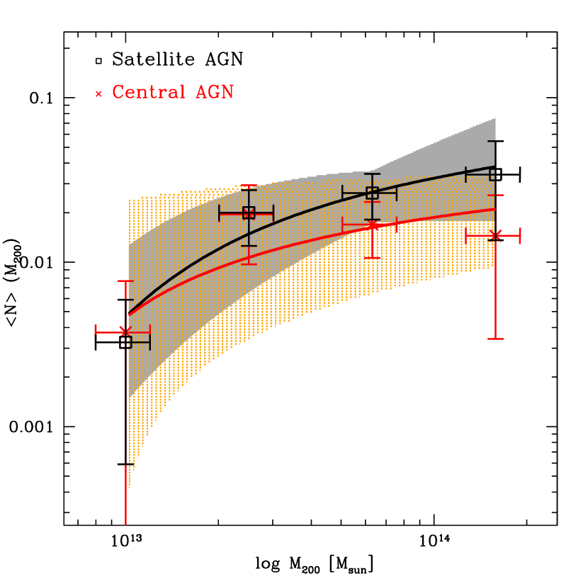
Figure 5.— Occupation of galaxy groups by satellite AGN (black squares) and central AGN (red crosses) as a function of the halo mass when correcting for the redshift evolution of the AGN density and for the soft XLF. The fit assuming a rolling-off power-law dependence is shown as solid black line (best fit) and dashed grey region ($1\sigma$ confidence interval) for AGN among satellite galaxies. The HOD for central AGN has been modelled with a softened step function (solid red line) where the shaded orange region marks the 68.3% confidence level.

The ACF is estimated by using the minimum variance estimator described by Landy & Szalay (1993):

$$\xi(r_{p},\pi)=\frac{DD-2DR+RR}{RR}$$ (11)

where DD, DR and RR are the normalized number of data-data, data-random, and random-random source pairs, respectively. Eq. 11 indicates that an accurate estimate of the distribution function of the random samples is crucial in order to obtain a reliable estimate of $\xi(r_{p},\pi)$. Several observational biases must be taken into account when generating a random sample of AGN in a X-ray flux limited survey. In particular, in order to reproduce the selection function of the survey, one has to carefully reproduce the space and flux distributions of AGN, since the sensitivity in X-ray surveys is not homogeneous on the detector and therefore on the sky. An other important choice for obtaining a reliable estimate of $w_{p}(r_{p})$, is to set $\pi_{max}$ in the calculation of the integral above. One should avoid values of $\pi_{max}$ too large since they would add noise to the estimate of $w_{p}(r_{p})$. If, instead, $\pi_{max}$ is too small one could not recover all the signal.

We created an AGN random sample where each simulated source is placed at a random position in the sky, with flux randomly extracted from the catalog of real source fluxes. The simulated source is kept in the random sample if its flux is above the sensitivity map value at that position (Miyaji et al., 2007; Cappelluti et al., 2009). The corresponding redshift for a random object is assigned based on the smoothed redshift distribution of the AGN sample.

Similarly, an unclustered catalog of galaxy groups mimicking the selection function of the survey must be employed to quantify the degree to which the groups preferentially locate themselves in one another’s neighborhood. We generate a random group catalog by calculating at each area of a given sensitivity, the probability of observing a group of a given mass and redshift. We then used Monte-Carlo simulation of the group positional assignment, finally producing a catalog of hundred thousand objects. Also the X-ray surface brightness sensitivity map is non-uniform in depth and consequently the probability of detecting groups of a particular mass is variable with redshift; in particular the minimum mass below which a group will be detected is an increasing function of $z$.

4.2. Galaxy Groups ACF

We measured the projected ACF of galaxy groups in the range $r_{p}=0.1-40$ h^-1Mpc by using Eq. 10, with $\pi_{max}=80$ h^-1Mpc (see Fig.6). The errors have been estimated using bootstrap resampling of the data, which consists of computing the variance of $w_{p}(r_{p})$ in $N_{real}$ bootstrap realizations of the sample. Each realization is obtained by randomly selecting a subset of groups from the data sample allowing for repetitions.

In the halo model approach, the clustering signal can be modelled as the sum of two contributions of pairs from the same DM halo (1-halo term) and those from different DM halos (2-halo term). In Fourier space, the 2-halo term can be explicitly written as (Seljak 2000, Cooray & Sheth 2002):

$$P_{2-h}\approx b^{2}P_{lin}(k,z)$$ (12)

where $P_{lin}(k,z)$ is the linear power spectrum and $b$ is the bias factor of the sample. Then the galaxy groups two-point correlation function at large scales is given by:

$$w_{p,2-h}(r_{p})=b_{group}^{2}\int\frac{k}{2\pi}P_{lin}(k)J_{0}(kr_{p})dk$$ (13)

where $J_{0}(x)$ is the zeroth-order Bessel function of the first kind. Following this model, the galaxy group bias defines the relation between the 2-halo term of DM and groups clustering signal:

$$b^{2}_{group,obs}(r_{p})=\frac{w_{p,2-h}(r_{p})}{w_{DM}^{2-h}(r_{p},z=0)}$$ (14)

According to this equation, we estimated an average bias factor in the range $r_{p}=1-40$ h^-1Mpc equal to $b_{group,obs}=2.20\pm 0.12$ where the error corresponds to $\Delta\chi^{2}=1$ using a $\chi^{2}$ minimization technique with 1 free parameter. Following the bias mass relation $b(M_{h},z)$ described in van den Bosch (2002) and Sheth et al. (2001), this observed bias, with respect to the DM distribution at $z=0$ corresponds to a typical mass log$M_{typ}$ [h${}^{-1}M_{\odot}$] = 13.65${}^{+0.07}_{-0.08}$.

Figure 6.— :Upper Panel: Projected auto-correlation function of galaxy groups with $z\leq 1$. Following the halo model approach, the clustering signal at large scale ($r_{p}>1-2h^{-1}$ Mpc) is produced by separate DM halos (so called 2-halo term) and it can be expressed as $b_{group}^{2}w_{DM}^{2-h}(r_{p},z=0)$ (dotted line), where the bias factor is defined in Equation 15. Lower Panel: Bias factor versus $r_{p}$. The solid line shows the best-fitting constant value. The shaded regions indicate the values of the bias for which $\Delta\chi^{2}=1$ (dashed line) and $\Delta\chi^{2}$ = 4 (dotted lines).

On the other hand the average bias of galaxy groups can be estimated starting from the known masses $M_{200}$. Since usually the bias factor is related to the average DM halo mass expressed in units of $h^{-1}M_{\odot}$, hereafter we refer to $M_{h}$ to indicate the galaxy groups masses in these units. Since we know the mass estimates, we can predict the bias factor of this sample of galaxy groups. By accounting for the fact that the linear regime of the structure formation is verified only at large scales, we estimated the average bias of the sample, including only pairs which contribute to the clustering signal at $r_{p}=1-40$ Mpc $h^{-1}$. As described in Allevato et al. (2011), we measured the average bias factor of the sample as:

$$b_{group}(M_{h})=\sqrt{\frac{\sum_{i,j}b_{group,i}b_{group,j}D_{i}D_{j}}{N_{pairs}}}$$ (15)

where $b_{gg,i}b_{gg,j}$ is the bias factor of the group pair $i-j$ and $N_{pairs}$ is the total number of group pairs in the range $r_{p}=1-40$ Mpc $h^{-1}$. The $D$ factor is defined by $D_{1}(z)/D_{1}(z=0)$, where $D_{1}(z)$ is the growth function (see eq. (10) in Eisenstein & Hu (2001) and references therein) and takes into account that the amplitude of the DM 2-halo term decreases with increasing redshift.
By using this approach we obtained $b_{group}=2.21^{+0.13}_{-0.14}$ where the errors have been estimated assuming a $20\%$ error on the galaxy groups masses. This value is in perfect agreement with the bias obtained from the ACF, with $b_{group}/b_{group,obs}=1.00\pm 0.05$.

4.3. X-ray AGN-Galaxy Groups Cross-Correlation

Measurements of the cross-correlation function between AGN and groups use a version of the estimator proposed by Landy & Szalay (1993):

$$\xi=\frac{1}{R_{g}R_{A}}(D_{g}D_{A}-D_{g}R_{A}-D_{A}R_{g}+R_{g}R_{A})$$ (16)

where each data sample, with pair counts $D_{i}$ has an associated random catalog, with pair counts $R_{i}$ normalized by its number density.

We estimated the cross-correlation function of 189 galaxy groups and a subset of 253 XMM-COSMOS AGN with known spectroscopic redshift $\leq 1$, obtained excluding those within $R_{200}$ (see Fig. 7).

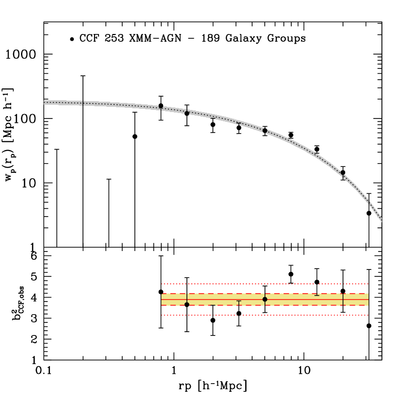
Figure 7.— : Upper Panel: Projected cross-correlation function of 253 XMM-COSMOS AGN with $z_{spec}\leq 1$ and 189 galaxy groups, excluding from the analysis AGN that are within in galaxy groups. The clustering signal at large scale $r_{p}>1-2h^{-1}$ Mpc is due to AGN residing in different DM halos and is described by $b_{CCF}^{2}w_{DM}^{2-h}(r_{p},z=0)$ (dotted line), where the bias factor is defined in Equation 17. On the contrary the 1-halo term is zero since we are removing from the analysis AGN with $R_{200}$ responsible for the signal of AGN within the same DM halos. Lower Panel: Bias factor versus $r_{p}$. The solid line shows the best-fitting constant value. The shaded regions indicate the values of the bias for which $\Delta\chi^{2}=1$ (dashed line) and $\Delta\chi^{2}$ = 4 (dotted lines).

Following Eq. 13, the linear bias factor of the projected CCF of AGN with galaxy groups can be approximated by using the 2-halo term:

$$b^{2}_{CCF,obs}(r_{p})=b_{AGN}(r_{p})b_{group}(r_{p})=\frac{w_{p,2-h}^{CCF}(r_{p})}{w_{DM}(r_{p},z=0)}$$ (17)

where $b_{AGN}$ and $b_{group}$ are the bias factor of AGN and galaxy groups, respectively and $w_{DM}$ is the projected dark matter CF. Fig. 7 (Lower Panel) shows the linear bias $b_{CCF}^{2}$ as a function of $r_{p}$ over the scales $r_{p}\sim 1-40$ h^-1Mpc. We fitted the data points with a constant by using the $\chi^{2}$ minimization technique and we found $b^{2}_{CCF,obs}=3.90\pm 0.28$. The shaded regions show the bias values for which $\Delta\chi^{2}$=1 and 4 (68% and 99% confidence levels for one parameter).

5. The bias factor in the HOD model

Based on the halo model approach, the AGN bias factor depends on the mean AGN HOD $\langle N_{AGN}\rangle(M_{h})$:

$$b_{AGN}(z)=\frac{\int_{M_{min}}^{\infty}b_{h}(M_{h},z)\langle N_{AGN}\rangle(M_{h})n_{h}(M_{h},z)dM_{h}}{\int_{M_{min}}^{\infty}\langle N_{AGN}\rangle(M_{h})n_{h}(M_{h},z)dM_{h}}$$ (18)

where $M_{min}$ is the minimum mass below which the AGN HOD is zero, $n_{h}(M_{h})$ and $b_{h}(M_{h})$ are the halo mass function and the halo bias given by Sheth et al. (2001). Note that the large-scale bias factor does not depend on the normalization log$M_{1}[M_{\odot}]=10^{13.8}$ and on $f_{a}$. Since we are estimating the CCF excluding from the XMM-COSMOS sample 41 AGN in galaxy groups, the clustering signal at large scale is due to AGN that live in halos with $M_{200}<10^{13}M_{\odot}$ or with masses that we can not observe at a given redshift $z$. This implies that the AGN bias can be written as:

$$b_{AGN}(z)=\frac{\int_{M_{min}}^{M_{x}(z)}b_{h}(M_{h},z)\langle N_{AGN}\rangle(M_{h})n_{h}(M_{h},z)dM_{h}}{\int_{M_{min}}^{M_{x}(z)}\langle N_{AGN}\rangle(M_{h})n_{h}(M_{h},z)dM_{h}}$$ (19)

where $M_{x}(z)$ is the minimum mass we can observe for a group at redshift $z$ (at $z\sim 1$ we only detect luminous and then massive groups). Note that we are assuming the separability of the mass and redshift dependence of the $\langle N_{AGN}\rangle$, i.e. $\langle N_{AGN}\rangle(M_{h},z)=\langle N_{AGN}\rangle(M_{h},z=0)\times\langle N_{AGN}\rangle(z)$.

Following this method, the bias factor $b^{2}_{CCF}$ is defined by:

$$b^{2}_{CCF}=\frac{\sum_{i,j}b_{AGN,i}b_{group,j}D_{i}D_{j}}{N_{pairs}}$$ (20)

where the sum is over the pairs $i,j$ contributing to the clustering signal at large scale and $b_{AGN}(z_{i})$ is the AGN bias (Eq. 19) assuming a rolling-off power-law HOD based on our results. $b_{group,j}$ is the bias associated to the galaxy group mass and redshift following Sheth et al. (2001) and $N_{pairs}$ is the total number of AGN-group pairs in the range $r_{p}=1-40$ h^-1Mpc. We found $b^{2}_{CCF}=3.97^{+0.10}_{-0.05}$, which is in perfect agreement with the observed bias factor defined in Eq. 17. The errors are due to the $1\sigma$ errors on the power-law index $\alpha$, $M_{min}$ and on $b_{group}$.

Similarly we can define the average halo mass $\langle M\rangle$ corresponding to the observed CCF signal, i.e.:

$$\langle M\rangle=\frac{\sum_{i,j}b_{AGN,i}b_{group,j}D_{i}D_{j}M_{h}^{i,j}}{\sum_{i,j}b_{AGN,i}b_{group,j}D_{i}D_{j}}$$ (21)

where $M_{h}^{i}(z_{i})$ is the average AGN host halo mass at redshift $z_{i}$:

$$M_{h}^{i}(z_{i})=\frac{\int_{M_{min}}^{M_{x}(z)}\langle N_{AGN}\rangle(M_{h})n_{h}(M_{h},z_{i})M_{h}dM_{h}}{\int_{M_{min}}^{M_{x}(z)}\langle N_{AGN}\rangle n_{h}(M_{h},z_{i})dM_{h}}$$ (22)

while $M_{h}^{j}(z_{j})$ is the galaxy group mass, both in units of h${}^{-1}M_{\odot}$. Fixing the values of $\alpha$ and $M_{min}$, we found the average mass of XMM-COSMOS AGN to be $log\langle M\rangle$ [h${}^{-1}M_{\odot}$]= 13.20(13.10;13.25), where the errors correspond to the 68% confidence region in the log$M_{min}-\alpha$ space.

6. Discussion

Using a sample of X-ray selected AGN and galaxy groups in the COSMOS field at $z\leq 1$, we performed the first direct measurement of the AGN HOD in the mass range $logM_{200}=13-14.5M_{\odot}$, based on the mass function of galaxy groups hosting AGN. In contrast to previous works using the clustering signal of the sample, we directly counted the number of AGN within galaxy groups and we found 58 AGN in groups, associated to 22 central and 36 satellite galaxies. This allowed us to put constrains on both the mean occupation of AGN among satellite and central galaxies as function of the halo mass, which provides information on the AGN triggering mechanism. Starikova et al. (2011) studied the halo occupation properties of AGN detected by the Chandra X-ray Observatory in the Bootes field over a redshift interval from z=0.17 to z=3, showing that X-ray AGNs are predominantly located at the centers of DMHs with $M_{h}>4.1\times 10^{12}$ h${}^{-1}M_{\odot}$, with an upper limit of the satellite fraction of 0.1 ($\Delta\chi^{2}<2.3$). The central locations of the quasar host galaxies are expected in major merger models because mergers of equally sized galaxies preferentially occur at the centers of DMHs (Hopkins et al. 2008). On the contrary Padmanabhan et al. (2009) observed the presence of the one-halo term in the cross-correlation function of optically selected $z<0.6$ quasars and Luminous Red Galaxies, and use this to conclude that a large fraction of the AGNs is hosted by satellite galaxies.

Our results show that the average number of AGN in satellite galaxies in the halo mass range $logM_{h}[M_{\odot}]=13-14.5$, and AGN luminosity $log\langle L_{X}\rangle$ [erg s^-1]= 42.3 might be comparable or even larger that the average number of AGN in central galaxies, i.e. X-ray AGN do not avoid satellite galaxies. A high fraction of AGN in satellite galaxies is expected in a picture where other phenomena like secular processes, might become dominant in the AGN activation. Milosavljevic et al. (2006), Hopkins & Hernquist (2006) and Hopkins & Hernquist (2009) showed that low-luminosity AGN could be triggered in more common nonmerger events, like stochastic encounters of the black holes and molecular clouds, tidal disruption or disk instability. This leads to the expectation of a characteristic transition to merger-induced fueling around the traditional quasar-Seyfert luminosity division.

Moreover we found the power-law slope, which defines the evolution of the mean satellite HOD with halo mass, to be $\alpha_{s}\sim 0-0.6$, suggesting a picture in which the average number of satellite AGN per halo increases with the halo mass. On the other hand, Miyaji et al. (2011) obtained $\alpha_{s}<0.95$, but negative values of the slope are not rejected ($\Delta\chi^{2}<2.3$).

It is interesting to compare this result with HOD analyses of galaxies. Previous HOD analyses of galaxies found $\alpha_{s}\sim 1-1.2$ for a wide range of absolute magnitudes and redshifts at least up to $z\sim 1.2$ (Zehavi et al., 2005; Zheng et al., 2007; Zehavi et al., 2010), implying a simple proportionality between halo mass and satellite number, $\langle N_{sat}\rangle\propto M_{h}$. Our results suggest that the mean HOD of satellite AGN might increase slower ($\alpha_{s}<0.63$) with the halo mass respect to the linear proportion ($\alpha_{s}=1$) in the satellite galaxy HOD, i.e. the AGN is not only triggered by the halo mass. On the contrary, a decreasing AGN fraction with the halo mass is consistent with previous observations that the AGN fraction is smaller in clusters than in groups in the nearby universe.

In order to fully understand the growth history of SMBHs as well as the physical processes responsible for the AGN activity we need to explore the AGN HOD at different redshifts, luminosities, and AGN types. The luminosity distribution of AGN that reside in halos of a given mass provides a tool to examine the distribution of halo mass for a given luminosity and study luminosity dependent clustering. While this formalism has been widely used in modelling galaxy clustering, it is still not applicable to AGN. In fact, it is also important to have larger numbers of AGN in galaxy groups which will enable stronger constraints on the shape of the satellite and central AGN HOD, hopefully as function of AGN luminosity and redshift.

7. Conclusions

We have performed the first direct measurement of the mean halo occupation distribution of X-ray AGN as function of halo mass, by directly counting the number of AGN within X-ray galaxy groups with masses $logM_{200}[M_{\odot}]=13-14.5$, in the COSMOS field at $z\leq 1$. Our findings are summarized as follows.

1. We identified 41 XMM-COSMOS AGN within galaxy groups, defined as AGN located within 3 times the group line-of-sight velocity dispersion and within $R_{200}$ and 17 additional sources including in the analysis C-COSMOS only selected AGN.

2. We measured the mean AGN occupancy of galaxy groups as function of halo mass in the range log$M_{200}[M_{\odot}]=13-14.5$ and we modelled the data points with a rolling-off power-law with the best fit index $\alpha=0.06(−0.22,0.36)$ and normalization parameter $f_{a}=0.05(0.04,0.06)$.

3. Using a galaxy membership catalog, we associated 22/58 and 36/58 AGN to central and satellites galaxies, respectively. We constrained that the mean AGN occupation function among central galaxies is described by a softened step function above log$M_{min}=12.75(12.10,12.95)$ while the satellite AGN HOD increases with the halo mass ($\alpha_{s}<0.63$) slower than the satellite HOD of sample of galaxies ($\alpha_{s}=1-1.2$).

4. We presented an estimate of the projected ACF of galaxy groups over the range $r_{p}=$ 0.1-40 h^-1Mpc at $\langle z\rangle=0.5$. We verified that the bias factor and the corresponding typical halo mass estimated from the observed galaxy group ACF, are in perfect agreement with the values $b_{group}$ and $\langle M_{h}\rangle$ obtained by using the galaxy group mass estimates. In particular we found $b_{group}=2.21^{+0.13}_{-0.14}$ and log $\langle M_{h}\rangle$ [h${}^{-1}M_{\odot}$] = 13.61${}^{+0.09}_{-0.10}$,

Table 2AGN in galaxy groups

$ID$	Ra	Dec	$z$	log$M_{200}$	$ID$	AGN Ra	AGN Dec	$ID$	$z$	$logL_{X}$	Flag
Groups	deg	deg	Groups	[$M_{\odot}$]	$XMM$	deg	deg	$Chandra$	AGN	[$h^{-2}_{70}$ erg $s^{-1}$]
11	150.1898	1.65725	0.22	14.28	-99	150.19864	1.671924	12390	0.228∗	41.27	0
17	149.96413	1.68033	0.372	14.02	30744	149.96396	1.6805983	-99	0.372	43.28	1
19	150.37282	1.60944	0.103	12.98	2021	150.37256	1.6093965	1678	0.104	41.22	1
20	150.32494	1.60313	0.22	13.38	2186	150.33601	1.6012201	1671	0.234∗	41.88	0
35	150.2066	1.82327	0.53	13.70	-99	150.20702	1.823398	1292	0.529	41.73	1
39	149.82381	1.8252701	0.531	13.63	5502	149.81248	1.8238187	219	0.529	42.37	0
52	150.44704	1.8828501	0.671	13.64	30681	150.44731	1.8832886	690	0.670∗	42.75	1
69	150.42012	1.9708	0.862	13.49	5519	150.42473	1.9693011	1185	0.854∗	42.77	0
78	150.27461	1.98884	0.838	13.61	-99	150.27823	1.990302	685	0.838	42.35	1
78	150.27461	1.9888	0.838	13.61	206	150.27434	1.9884306	1100	0.673	42.57	0
79	150.44728	2.05392	0.323	13.77	-99	150.44765	2.053961	2605	0.323	41.62	1
87	150.51109	2.0269899	0.899	13.60	2387	150.51036	2.0293686	496	0.899	43.15	1
93	149.6692	2.0740	0.338	13.59	417	149.6692	2.073962	168	0.34	42.76	0
110	150.17979	2.1103699	0.361	13.43	6	150.17978	2.1101542	42	0.360	43.19	1
118	149.63463	2.1357	0.962	13.70	411	149.63828	2.1494889	323	0.952	43.25	0
124	150.05656	2.2085	0.186	13.22	302	150.0571	2.2063098	1297	0.186	41.25	0
124	150.05656	2.20854	0.186	13.22	-99	150.09554	2.2202671	1221	0.186	40.86	0
128	150.58435	2.1811	0.556	13.58	2855	150.57634	2.1812408	1634	0.554	42.41	0
127	150.44104	2.15873	0.377	13.32	-99	150.44202	2.1551671	2313	0.376	41.24	1
130	150.02382	2.2032	0.942	13.84	-99	150.02303	2.206567	2413	0.94	42.45	0
136	150.17493	2.2170	0.676	13.56	-99	150.17592	2.2156539	877	0.667∗	42.08	0
137	149.96271	2.2102399	0.425	13.32	-99	149.96216	2.2102211	12011	0.425	41.44	1
138	149.50874	2.2614	0.943	13.97	5539	149.50914	2.261276	-99	0.962	43.19	1
142	150.28798	2.2769	0.122	13.09	317	150.25331	2.2779887	3718	0.165	41.08	0
143	150.21454	2.2801	0.880	13.77	116	150.20604	2.2857771	22	0.874	43.33	0
149	150.41566	2.4302	0.124	13.85	45	150.33598	2.4335926	658	0.121	41.31	0
149	150.41566	2.4302001	0.124	13.85	73	150.416	2.4299896	634	0.124	42.00	1
161	149.95262	2.3418	0.941	13.74	430	149.95949	2.3560882	497	0.889	42.85	0
171	149.66328	2.2677	0.676	13.56	5411	149.66243	2.2693584	1646	0.676	42.76	0
173	150.05804	2.38045	0.347	13.48	241	150.05794	2.3805208	898	0.347	42.14	1
174	149.63988	2.3491	0.950	13.97	53937	149.64459	2.3587193	-99	0.962∗	42.88	0
175	150.24123	2.34835	0.723	13.55	-99	150.24109	2.3483839	977	0.703	41.72	0
186	150.21748	2.4003	0.905	13.77	53303	150.21141	2.4022212	975	0.894∗	42.62	0
194	149.69957	2.4028	0.354	13.45	135	149.70084	2.4025679	417	0.376	43.00	0
196	150.27898	2.4192	0.123	13.11	-99	150.27975	2.4222209	1315	0.122	40.25	0
216	150.06664	2.6474	0.696	13.64	5113	150.06633	2.642817	143	0.693	42.45	0
217	150.00713	2.4534299	0.731	13.54	-99	150.00188	2.4606521	1243	0.732	42.39	1
219	150.27148	2.5134399	0.704	13.54	158	150.27411	2.5117824	138	0.703	42.51	1
220	149.92343	2.5249	0.729	14.39	486	149.92007	2.5143571	562	0.698	42.52	0
220	149.92343	2.5249901	0.729	14.39	-99	149.91588	2.52139	1310	0.729	42.38	0
231	150.05421	2.58885	0.675	13.73	8	150.05383	2.5896702	142	0.699	44.03	1
234	150.15816	2.6082	0.893	13.66	-99	150.15796	2.6113441	727	0.863∗	42.35	0
237	150.11774	2.6842501	0.349	14.00	5118	150.11783	2.6840661	-99	0.349	42.18	1
259	149.65717	2.8195	0.703	13.73	60270	149.65953	2.8270493	-99	0.708∗	42.33	0
262	149.60007	2.8211	0.344	14.03	5320	149.63142	2.8174951	-99	0.34	42.93	0
275	149.83878	2.6750801	0.259	13.45	5112	149.83847	2.6750875	1608	0.259	43.08	1
277	150.00462	2.63275	0.677	13.45	5091	150.00452	2.6328416	616	0.678	42.73	1
289	150.11256	2.5560	0.501	13.57	142	150.10342	2.5504889	148	0.498	42.62	0
292	150.03307	2.5524	0.747	13.48	398	150.02638	2.5620575	991	0.745	42.82	0
296	149.55516	2.0020	0.894	13.90	10732	149.56131	2.0087938	3549	0.930∗	42.85	0
298	149.78191	2.1390	0.354	13.59	63	149.78223	2.1387713	313	0.355	42.57	0
298	149.78191	2.13906	0.354	13.59	392	149.79369	2.1256437	679	0.353	41.98	1
298	149.78191	2.13906	0.354	13.59	-99	149.77357	2.141633	1498	0.354	41.34	0
300	149.72893	2.2373	0.381	13.47	-99	149.74792	2.253087	2876	0.356	41.06	0
303	149.99364	2.2585399	0.660	13.53	19	149.99367	2.2585886	450	0.659	43.38	1
322	150.2254	2.26872	0.677	13.51	-99	150.228	2.2698331	24	0.678	42.46	0
324	150.02414	2.36050	0.726	13.39	254	150.03079	2.358371	533	0.786	42.89	0
333	150.0423	2.6949	0.219	13.31	5075	150.04155	2.6945302	623	0.221	41.46	1

References

- Allevato et al. (2011) Allevato V., et al. 2011, ApJ, 736, 99
- Avni & Bahcall (1980) Avni, Y. & Bahcall, J. N., 1980, ApJ, 235, 694
- Balogh et al. (2011) Balogh, M. L., et al. 2011, MNRAS, 412, 2303
- Berlind et al. (2003) Berlind A. A., et al. 2003, ApJ, 593, 1
- Bierly et al. (2010) Bierly, R. M., et al. 2010, A&A, 523, 66
- Bonoli et al. (2009) Bonoli, S., Marulli, F., Springel, V., et al. 2009, MNRAS, 396, 423
- Brusa et al. (2010) Brusa, M., Civano, F., Comastri, A., et al. 2010, ApJ, 716, 348
- Cappelluti et al. (2007) Cappelluti, N., et al. 2007, ApJS, 172, 341
- Cappelluti et al. (2009) Cappelluti, N., Brusa M., Hasinger G., et al. 2009, A&A, 497, 635
- Cappelluti et al. (2010) Cappelluti, N., et al. 2010, ApJ, 716, 209
- Cappelluti, Allevato & Finoguenov (2012) Cappelluti, N., Allevato, V., Finoguenov, A., Advances in Astronomy, vol. 2012, id. 853701
- Chatterjee et al. (2012) Chatterjee S., et al. 2012, MNRAS, 419, 2657
- Cisternas et al. (2011) Cisterans, M., et al. 2011, ApJ, 726, 57
- Civano et al. (2012) Civano, F., et al. 2012, ApJ, 752, 49
- Coil et al. (2009) Coil, A. L., Georgakakis, A., Newman, J. A., et al. 2009, ApJ 701 1484
- Cooray & Sheth (2002) Cooray, A., Sheth, R., 2002, PhR, 372, 1
- Croom et al. (2005) Croom, Scott M., Boyle, B. J., Shanks, T., Smith, R. J., et al. 2005, MNRAS, 356, 415
- Davis & Peebles (1983) Davis, M., Peebles, P. J. E., 1983, ApJ, 267, 465
- Dunlop et al. (2003) Dunlop J. S., McLure R. J., Kukula, M. J., et al. 2003, MNRAS, 340, 1095
- Ebrero et al. (2009) Dunlop J. S., McLure R. J., Kukula, M. J., et al. 2003, MNRAS, 340, 1095
- Elvis et al. (2007) Elvis, M., Chandra-COSMOS Team, 2007, in Bullettin of the American Astronomical Society, Vol. 39, p.899
- Elvis et al. (2009) Elvis M., et al. 2009, ApJS, 184, 158
- Eisenstein & Hu (2001) Eisenstein, Daniel J., Hu, Wayne., 1999, ApJ, 511, 5
- Finoguenov et al. (2007) Finoguenov, A., et al. 2007, ApJS, 172, 182
- Finoguenov et al. (2010) Finoguenov, A., et al. 2010, MNRAS, 403, 2063
- Fisher et al. (1994) Fisher, K. B., Davis, M., Strauss, M. A., Yahil, A. & Huchra, J., 1994, MNRAS, 266, 50
- Gabor et al. (2009) Gabor, J. M., et al. 2009, ApJ, 691, 705
- Georgakakis et al. (2007) Georgakakis, A., Nandra, K., Laird, E. S., et al. 2007, ApJ, 660, 15
- Georgakakis et al. (2009) Georgakakis, A., Coil, A. L., Laird, E. S., et al. 2009, MNRAS, 397, 623
- George et al. (2011) George, Matthew R., et al. 2011, ApJ, 742, 125
- George et al. (2012) George, Matthew R., et al. 2012, submitted
- Gilli et al. (2005) Gilli, R., Daddi, E., Zamorani, G., et al. 2005, A&A, 430, 811
- Gilli et al. (2009) Gilli, R., et al. 2009, A&A, 494, 33
- Grogin et al. (2005) Grogin, N. A., et al. 2005, ApJ, 627, 97
- Hamana et al. (2004) Hamana, T., Ouchi, M., Shimasaku, K., Kayo, I., & Suto, Y. 2004, MNRAS, 347, 813
- Hasinger et al. (2005) Hasinger, G., Hasinger, G., Schmidt, M., 2005, A&A, 441..417H
- Hasinger et al. (2007) Hasinger, G., et al. 2007, ApJS, 172, 29
- Hickox et al. (2009) Hickox, R. C., Jones, C., Forman, W. R., 2009, ApJ, 696, 891
- Hogg (1999) Hogg, D.W, 1999, arXiv:astro-ph/9905116
- Hopkins et al. (2007) Hopkins, P.F., et al. 2007, ApJ, 662, 110
- Hopkins et al. (2008) Hopkins, P.F., Hernquist, L., Cox, T.J., & Keres, D. 2008, ApJS, 175, 356
- Hopkins & Hernquist (2006) Hopkins, P.F., Hernquist, L., 2006, ApJ, 166, 1
- Hopkins & Hernquist (2009) Hopkins, P.F., Hernquist, L., 2009, ApJ, 694, 599
- Kauffmann, Nusser & Steinmetz (1997) Kauffmann, G., Nusser, A. & Steinmetz, M., 1997 MNRAS, 286, 795
- Kocevski et al. (2011) Kocevski, D. D., et al 2011, arXiv1109.2588K
- Kravtsov et al. (2004) Kravtsov A. V., et al. 2004, ApJ, 609, 35
- Krumpe et al. (2010) Krumpe, M., Miyaji, T., Coil, A. L. 2010, ApJ, 713, 558
- La Franca et al. (2005) La Franca, F., et al. 2005, ApJ, 635, 864
- Landy & Szalay (1993) Landy, S. D., & Szalay A. S., 1993, ApJ, 412, 64
- Leauthaud et al. (2010) Leauthaud, A., Finoguenov, A., Kneib, J. P., et al 2010, ApJ, 709, 97
- Leauthaud et al. (2007) Leauthaud, A., et al. 2007, ApJS, 172, 219
- Lilly et al. (2007) Lilly, S. J., Le Févre, O, Renzini, A, et al. 2007, ApJS, 172, 70
- Lilly et al. (2009) Lilly, S. J., Le Brun, V., Mayer, C., et al. 2009, ApJS, 184, 218
- Markevitch (1998) Markevitch, M., 1998, ApJ, 504, 27
- McIntosh et al. (2009) McIntosh, D. H., Guo, Y., Mo, H. J., van den Bosch, F., & Yang, 2009, Bulletin of the American Astronomical Society, 41, 423.09
- Miyaji et al. (2000) Miyaji, T., Hasinger, G., Schmidt, M., 2000, A&A, 353, 25
- Miyaji et al. (2007) Miyaji, T., Zamorani, G., Cappelluti, N., et al., 2007, ApJS, 172, 396
- Miyaji et al. (2011) Miyaji, T., Krumpe, M., Coil, A. L., & Aceves, H. 2011, ApJ, 726, 83
- Milosavljevic et al. (2006) Milosavljevíc, M., Merritt, D., & Ho, L. C. 2006, ApJ, 652, 120
- Mullis et al (2004) Mullis, C. R., Henry, J. P., Gioia, I. M., et al., 2004, ApJ, 617, 192
- Padmanabhan et al. (2009) Padmanabhan, N., White, M., Norberg, P., & Porciani, C. 2009, MNRAS, 397, 1862
- Pierce et al. (2007) Pierce, C. M., et al. 2007, ApJ, 660, 19
- Peacock & Smith (2000) Peacock, J. A., Smith, R. E. 2000, MNRAS318, 1144
- Phleps et al. (2006) Phleps S., Peacock J. A., Meisenheimer K., Wolf C. 2006, A&A, 457, 145
- Peebles (1980) Peebles P. J. E., 1980, The Large Scale Structure of the Universe (Princeton: Princeton Univ. Press)
- Porciani & Norberg (2006) Porciani, C., Norberg, P., 2006, MNRAS, 371, 1824
- Puccetti et al. (2009) Puccetti, S., et al. 2009, ApJS, 185, 586
- Reichard et al. (2009) Reichard, T. A., Heckmas, T. M., Rudnick, G., et al. 2009, ApJ, 691, 1005
- Rosario et al. (2011) Rosario, D. J., McGurk, R. C., Max, C. E., et al. 2011, 2011arXiv1102.1733R
- Richardson et al. (2012) Richardson, J., Zheng, Z., Chatterjee, S., NAgai, D., and Shen, Y., 2012, arXiv:1104.3550v2
- Ross et al. (2009) Ross, N. P., Shen, Y., Strauss, M. A., et al. 2009, ApJ, 697, 1634
- Salvato et al. (2011) Salvato, M., et al. 2011, ApJ, 742, 61
- Sanders et al. (2007) Sanders, D., Salvato, M., Aussel, H., et al. 2007, ApJS, 172, 86
- Schawinski et al. (2011) Schawinski, K,, Treister, E.,Urry, C. M., et al. 2011, ApJ, 727, 31
- Scoville et al. (2007) Scoville, N., Abraham, R. G., Aussel, H., et al. 2007, ApJS, 172, 38
- Shankar et al. (2009) Shankar, F., Weinberg D. H., et al. 2009, ApJ, 690, 20
- Shankar et al. (2010) Shankar F., et al., 2010, ApJ, 718, 231
- Shankar (2010) Shankar F., 2010, IAUS, 267, 248
- Shen et al. (2009) Shen Y., Strauss, M. A., Ross, N. P., Hall, P. B., et al. 2009, ApJ697, 1656
- Shen (2009) Shen Y., 2009, ApJ, 704, 89
- Shen et al. (2010) Shen, Y., et al. 2010, ApJ, 719, 1693
- Sheth et al. (2001) Sheth R. K., Mo H. J., Tormen G. 2001, MNRAS, 323, 1
- Silverman et al. (2009) Silverman, J. D.; Kovac̆, K., Knobel, C., ApJ, 695, 171
- Silverman et al. (2011) Silverman, J. D. et al. 2011, ApJ, 743, 2
- Starikova et al. (2011) Starikova, S. et al., 2011, ApJ, 741, 15
- Tal et al. (2009) Tal, T., van Dokkum P. G., Nelan, J., et al. 2009, ApJ, 138, 1417
- Taniguchi et al. (2007) Taniguchi, Y., Scoville, N. Z., Murayama, T., et al. 2007, ApJS, 172, 9
- Tinker et al. (2005) Tinker, J. L., Weinberg, D. H., Zheng, Z., Zehavi, I. 2005, ApJ, 631, 41
- Ueda et al. (2003) Ueda, Y., Akiyama, M., Ohta, K., & Miyaji, T., 2003, ApJ,598, 886
- Yang et al. (2006) Yang, Y., Mushotzky, R. F., Barger, A. J., & Cowie, L. L. 2006, ApJ, 645, 68
- van den Bosch (2002) van den Bosch, F. C. 2002, MNRAS, 331, 98
- Zamojski et al. (2007) Zamojski, M. A., Schiminovich, D., Rich, R. M., et al. 2007, ApJS, 172, 468
- Zehavi et al. (2005) Zehavi, I., et al. 2005, ApJ, 630, 1
- Zehavi et al. (2010) Zehavi, I., et al. 2010, arXiv:1005.2413
- Zheng et al. (2005) Zheng, Z., et al. 2005, ApJ, 633, 791
- Zheng et al. (2007) Zheng, Z., Coil, A. L., & Zehavi, I. 2007, ApJ, 667, 760
- Zheng et al. (2009) Zheng, Z., Zehavi, I., Eisenstein, D. J., Weinberg, D. H., & Jing, Y. P. 2009, ApJ, 707, 554