ZU-TH 19/12
LPN12-093
NLO QCD corrections to production in vector-boson fusion at the LHC
A. Denner1, L. Hošeková2 and S. Kallweit3
1 Universität Würzburg, Institut für Theoretische Physik und Astrophysik,
D-97074 Würzburg, Germany
2 Instituto de Física Corpuscular,
UVEG - Consejo Superior de Investigaciones Científicas,
E-46980 Paterna (Valencia), Spain
3 Institut für Theoretische Physik, Universität Zürich,
CH-8057 Zürich, Switzerland
Abstract:
We present a next-to-leading-order QCD calculation for production in vector-boson fusion, i.e. the scattering of two positively charged bosons at the LHC. We include the complete set of electroweak leading-order diagrams for the six-particle final state and quantitatively assess the size of the -channel and interference contributions in VBF kinematics. The calculation uses the complex-mass scheme to describe the W-boson resonances and is implemented into a flexible Monte Carlo generator. Using a dynamical scale based on the transverse momenta of the jets, the QCD corrections stay below about for all considered observables, while the residual scale dependence is at the level of .
September 2012
1 Introduction
Vector-boson fusion (VBF) processes at the Large Hadron Collider (LHC) offer unique signatures owing to two easily identifiable forward and backward jets. This process class is not only useful for confirming the existence of the Standard Model Higgs boson, but in particular for studying its characteristics, including its couplings to both fermions and electroweak (EW) vector bosons [1, 2] and its CP properties [3, 4].
VBF processes involving the scattering of vector bosons constitute an irreducible background to Higgs-boson production in association with two jets, in particular for decay modes as they share the same final states. It is therefore desirable to obtain accurate theoretical predictions and error estimates for these background processes. The reactions of the type are also seen as an important probe of the EW symmetry breaking itself [5]. Without the presence of the Higgs boson perturbative unitarity of the Standard Model at very high energy scales would be violated in processes involving weak-vector-boson scattering unless some other mechanism beyond that described by the Standard Model controls the unphysical behaviour (see e.g. Ref. [6]). Moreover, VBF into pairs of vector bosons is an important background to various searches for new physics.
We are specifically interested in VBF processes that involve the scattering of weak gauge bosons and lead to final states with two jets and four leptons (charged leptons and neutrinos). At leading order (LO), two hard production mechanisms give rise to these final states. The purely EW contributions of order involve in particular the genuine VBF contributions, i.e. diagrams where vector bosons are emitted from the incoming (anti-)quarks, then scatter and decay into pairs of leptons. In addition, there are QCD-production contributions of order which proceed via gluon-mediated (anti-)quark scattering processes or processes with two external gluons and two external (anti-)quarks, where in both cases the two EW vector bosons are emitted from the (anti-)quark line(s). Since the jets in the QCD production mode tend to be closer in rapidity than in the EW production mode, a cut requiring a large rapidity separation between these jets or more generally a central jet veto suppresses the QCD production mode by two orders of magnitude as demonstrated in Refs. [7, 8, 6]. Owing to the different colour structure of QCD and EW production modes, interference terms between these mechanisms are doubly suppressed at LO; they only appear at sub-leading colour and if all quarks are identical. In our calculation, we restrict ourselves to the EW production mode.
In this paper we focus on the process involving two jets, two positively charged leptons and two neutrinos in the final state, i.e. . This process leads to a distinct signature of same-sign high- leptons, missing energy and jets. Since no gluon-initiated processes contribute to this final state at LO, it has a comparably low SM cross section and thus is a good candidate to search for physics beyond the SM. New-physics signals involving same-sign leptons originate for instance in -parity-violating SUSY models [9], in di-quark production with decay of the di-quark to a pair of top quarks [10], or from the production of doubly-charged Higgs bosons [11]. Moreover, it constitutes a background to double parton scattering [12, 13, 14].
Since LO cross sections carry a large uncertainty, the calculation of the NLO corrections in the strong coupling is needed to obtain a reliable prediction. For the QCD-mediated contributions to , and later also for , NLO results were presented in double-pole approximation, i.e. including only diagrams with two resonant bosons, but leptonic decays with full spin correlations [15, 16, 17]. For the computation [15] has been subsequently implemented [18] into the POWHEG BOX [19, 20]. In a series of NLO calculations for vector-boson scattering processes in VBF [21, 22, 23, 24], NLO results for the EW production mode were given for the complete process in Ref. [24] including the full set of - and -channel diagrams (also those without resonant W bosons) while neglecting -channel diagrams and interferences between - and -channel contributions. Also this computation has recently been combined with a parton shower [8] using the POWHEG BOX.
In this work we present an independent calculation of the NLO QCD corrections to EW production including leptonic -boson decays and non-resonant diagrams. This constitutes the first independent check of the calculation in Ref. [24]. Moreover, we investigate the size of the -channel and interference contributions at LO.
The paper is organized as follows: In Section 2 we discuss technical aspects of the calculation, namely the organization of Feynman diagrams into building blocks (Section 2.1) and the evaluation of the NLO corrections (Section 2.2). Section 3 covers numerical checks and comparisons with previously published results. Finally, in Section 4 we present numerical predictions for the LHC at , while Section 5 contains our conclusions.
2 Elements of calculation
We have developed a general framework for the calculation of QCD corrections to vector-boson scattering reactions at hadron colliders [25], i.e. for EW processes of the form with 4 arbitrary (charged and/or neutral) leptons. In this section we sketch the ingredients and main features of the method.
Because the LHC experiments are conducted at TeV energies, fermion-mass effects are strongly suppressed and have been neglected. At the same time, only the two lighter generations of quarks (u, d, c and s) and leptons have been taken into account. In Ref. [26], the contribution of external b quarks to Higgs production via VBF has been found to be at the level of 2% if VBF cuts are applied (4% without VBF cuts). For the processes involved in our calculation, these contributions can be expected to be of similar size, if not even smaller: e.g. in the channel discussed in this paper, external bottom (anti-)quarks would show up only accompanied by non-diagonal CKM matrix elements and thus be entirely negligible. Further, it can be demonstrated [23] that the CKM matrix can be approximated by a unit matrix provided the interferences between different kinematic channels as well as the -channel contribution are negligible, which is verified in Section 4.
2.1 Structure of the diagrams and building blocks
For the calculation of the LO and NLO matrix elements of the processes we adopt a similar strategy as in Refs. [21, 22, 23, 24]. In order to deal with the large number of diagrams111For there are 93 diagrams at LO. At NLO, 430 loop and 346 counterterm diagrams contribute, while the basic partonic real-emission process contains 452 diagrams., we introduce generic building blocks from which the matrix elements can be constructed. The details of our approach differ, however, in many aspects from Refs. [21, 22, 23, 24].
For the class of processes , the Feynman diagrams can be divided into four generic categories, taking advantage of the fact that the EW and QCD parts of the diagrams are largely independent of one another. Figure 1 demonstrates four generic types into which all t-channel diagrams involved in our calculation can be categorized.
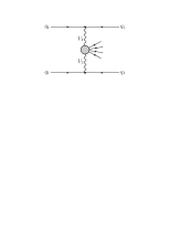
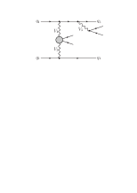
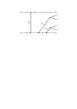
Type A (Figure 1a) represents the genuine VBF diagram, with two vector bosons radiated off the quark lines fusing in the centre to produce four leptons in the final state.
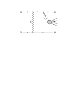
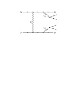
Type B (Figure 1b) contains two quark lines connected with a vector boson and another vector boson radiated off either of the two quark lines which decays via EW interactions into four final-state leptons. For combinatorial reasons, 4 topologies of this type exist.
Type C (Figure 1c) has a vector boson radiated off either one of the two quark lines which decays into two leptons, and two more vector bosons fusing in the central region to produce a second pair of leptons. Again, 4 topologies of this type exist.
Finally, type D (Figure 1d) sees one vector boson connecting the quark lines, and two more radiated either one off each quark line (diagram on the left) or both off the same quark line (diagram on the right) and subsequently decaying into two lepton pairs. In total, there are 10 different topologies of this type which are grouped together as they involve the same EW building blocks.
Each generic diagram involves two QCD parts—the two quark lines with attached vector bosons—and one or two EW parts, namely the vector-boson scattering block and/or vector-boson decays into leptons. Owing to charge conservation, not all generic topologies give rise to Feynman diagrams once particular insertions for the external (anti-)quarks, the final-state leptons, and, correspondingly, the intermediate EW bosons are fixed. Thus, for instance, type B is completely absent if the final-state lepton charges add up to .
Evidently changes to either QCD or EW parts that do not alter the momenta of the internal vector bosons have no effect on the rest of the diagram. For instance, application of crossing symmetry to the upper quark line does not influence the lower quark line and all leptonic parts. Similar arguments hold for adding a gluon loop to either of the quark lines, which essentially amounts to calculating virtual NLO QCD corrections to the entire diagram. Since the leptonic sector of the diagram in itself can be quite complicated, it is advantageous to calculate these blocks only once and reuse them with different QCD parts.
The calculation is performed in the ’t Hooft–Feynman gauge. Diagrams with would-be Goldstone bosons connecting EW and QCD parts do not contribute because their couplings to massless fermions vanish.222Note that would-be Goldstone bosons show up inside the EW vector-boson scattering building block of Figure 1a, namely in all processes involving a vertex. Factorization of parts of the diagrams can be achieved by inserting the polarization sums for massive vector bosons,
| (2.1) |
for the numerators of the gauge-boson propagators coupled to a quark line, effectively thus cutting the diagram into blocks that can be evaluated on their own. The polarization vectors and for off-shell particles are obtained by replacing the vector-boson mass with in the definition of the longitudinal polarization vector, i.e.
| (2.2) |
The polarization vectors do not depend on the mass and thus remain unchanged. Introducing
| (2.3) |
to compactify the notation, the polarization sum (2.1) can be rewritten as
| (2.4) |
Because of gauge invariance the contractions of with some of the building blocks vanish. After checking numerically that these terms do not contribute, we have omitted them in those type D diagrams (Figure 1d) in which two outgoing vector bosons couple to the same quark line since their evaluation consumes most CPU time (in comparison to the remaining topologies), particularly at NLO.
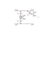
Implementing the block structure by cutting all internal vector bosons that couple to the quark lines in the diagrams in Figure 1 allows us to not only save CPU time by evaluating each required block only once, but also to keep the number of required blocks relatively small by reusing them in multiple instances throughout all diagrams and even partonic processes. The diagrams we need to consider in our calculation contain up to three vector bosons that are being radiated off the quark lines, and the polarization sum has to be applied once to each of their propagators. Figure 2 illustrates how a diagram featuring three vector bosons can be split into four building blocks. Each splitting represents an insertion of one polarization sum. The resulting amplitude reads:
| (2.5) |
where are the denominator parts of the gauge-boson propagators, and , , and , according to the notation introduced in Figure 2.
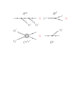


Building blocks involving leptons (shown in Figure 3) typically involve more than one Feynman diagram, with the exception of the block corresponding to the EW current (Figure 3a). Diagrams of type B (Figure 1b) contain building blocks with one vector boson in the initial state and four leptons in the final state (Figure 3b). Building blocks with two external vector bosons (Figures 3c and 3d) are represented by a array, each element corresponding to one term of the complete polarization sum constructed by cutting the two vector bosons.
At LO, the QCD building blocks are formed by one diagram each, as shown in Figure 4. Blocks involving two vector bosons entering diagrams of type B, C and D are represented by a array (Figure 4b). Building blocks with three outgoing vector bosons (Figure 4c) appearing in type D are represented by arrays.
| : | : | |||
| : | ||||
| : | ||||
| : | ||||
| : | ||||
All partonic processes contributing to a specific process can be constructed from up to 8 generic -channel matrix elements listed in Table 1 (e.g. for ) by applying crossing symmetry to reverse the flow of either one or both quark currents (e.g. ) and to construct the -channel diagrams (e.g. ), or by exchanging the outgoing lines to obtain -channel diagrams (e.g. ). As the order of the outgoing partons is obviously arbitrary, the distinction between - and -channel diagrams only makes sense if both types contribute to the same partonic process (e.g. ), which is the case if all (anti-)quarks belong to the same generation.
With the CKM matrix approximated by a unit matrix, partonic processes which result from one another by interchanging all first-generation (anti-)quarks with their second-generation counterparts and vice versa, are described by the same matrix elements. For instance, the partonic processes and only differ in the parton distribution functions, and the matrix element can be recycled. Analogously, partonic processes involving two different generations of quarks—for example and —are pairwise formed by identical matrix elements.
In our calculation, the formulae for combining the blocks have been implemented as Fortran subroutines. The expressions for the individual building blocks are obtained by means of the FormCalc 6 package [27], which also introduces abbreviations for the fermion chains and thus helps to speed up the code significantly. They are evaluated using the Weyl–van der Waerden (WvdW) helicity formalism [28] allowing us to express all subamplitudes involved in the polarization sums in terms of universal WvdW spinors and compute them numerically. The FormCalc code is modified to transform the amplitudes to the form (2.1), further abbreviations of spinor products are introduced, and each building block is exported into a Fortran module which takes the momenta and helicities for the particles in the building block as input. The Fortran code for each process is contained in a single function that can be called from within a Monte Carlo program and returns an array of full squared amplitudes for each partonic process, including all relevant colour and averaging factors.
2.2 Calculation of NLO cross sections and matrix elements
Cross sections involving two initial-state hadrons at a fixed perturbative order are given as a convolution of the parton distribution functions (PDFs) and the partonic cross sections , summed over all incoming partons resulting in contributions to the considered hadronic process.
At LO, the cross section is defined by
| (2.6) |
where are the PDFs that give the probability to find parton with a momentum fraction in the respective proton, is the differential partonic Born cross section which is integrated over the -parton phase-space . While the sum over the incoming partons and is explicitly stated, summation over all outgoing parton configurations giving rise to non-vanishing partonic contributions to the hadronic process discussed is implicitly assumed.
At NLO QCD, virtual and real corrections contribute to the cross section, which separately contain soft and collinear divergences. However, these infrared (IR) divergences cancel in the NLO cross section, if IR-safe jet observables are considered and the PDFs are renormalized appropriately. For mediating this cancellation, the Catani–Seymour dipole-subtraction technique for massless particles [29] is applied. This procedure allows us to express the NLO cross section as a sum over individually finite phase-space integrals,
with the conventions of (2.6). The differential partonic contributions and correspond to the virtual and real corrections, respectively. The process-independent operators , , and are defined in Ref. [29], and symbolizes the colour correlations between Born matrix elements and these operators (spin correlations do not appear in the given process class as no external gluons are involved at Born level). In the processes , the Born and virtual cross sections are built from the partonic initial states , while in the real cross section additionally contribute.
The process-dependent ingredients which are necessary for calculating the NLO cross sections of the processes are thus:
-
1.
Born-level level matrix elements needed for , evaluated in four dimensions. Their construction is outlined in the previous section.
-
2.
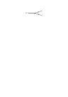
One-loop virtual matrix elements needed for , with renormalized ultraviolet divergences and IR divergences regularized using dimensional regularization, evaluated in dimensions. Once the QCD and EW sections of the diagrams are separated, the transition from LO to virtual corrections can be performed by adding a gluon loop to either of the two quark lines. Continuing with the example in Figure 2, one of the building blocks or is replaced by or (shown in Figure 5) respectively, while the other one remains unchanged. The ultraviolet divergences are renormalized by adding the corresponding counterterms. Since neither of these changes has any influence on the overall kinematics of the diagram, the leptonic blocks and stay the same as in the LO.
-
3.
Real-radiation matrix elements needed for , evaluated in four dimensions. They can be created in a similar manner as in the LO case. In the example from Figure 2, this amounts to attaching an outgoing gluon in every possible way in the building blocks or and shifting the momenta , and of the intermediate vector bosons accordingly. The diagrams with an initial-state gluon can then be obtained via crossing symmetry.
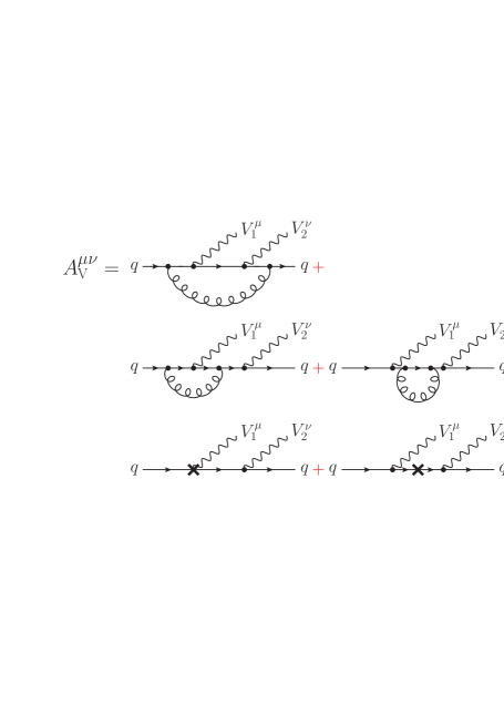
Figure 5: Virtual contributions and corresponding to building blocks and in Figure 2. -
4.
A set of colour projected Born-level matrix elements required to construct and , evaluated in four dimensions. In the VBF approximation of the matrix elements (no -channel diagrams and no interferences between - and -channel diagrams), the colour correlations turn out to be trivial and give rise to the same constant factor for all colour-correlated Born matrix elements.
Analytical expressions for the virtual amplitudes have been generated in the same way as for the Born amplitudes. All divergences of the loop diagrams appear in tensor integrals, which are given by two, three, four and five-point functions. In our calculation, the tensor reduction is performed numerically in Fortran by means of the COLLIER library [30, 31, 32, 33, 34, 35] which is based on the tensor reduction scheme developed by Denner and Dittmaier [30, 31] and supports both mass and dimensional regularization scheme.
The resonant bosons require a proper inclusion of the finite vector-boson widths in the propagators. We use the complex-mass scheme, which was introduced in Ref. [36] for LO calculations and generalized to the one-loop level in Ref. [37]. In this approach, the W- and Z-boson masses as well as the Higgs-boson mass are consistently considered complex quantities, defined as the locations of the propagator poles in the complex plane. This leads to complex couplings and, in particular, a complex weak mixing angle. The scheme fully respects all relations that follow from gauge invariance. A brief description of the complex-mass scheme can also be found in Ref. [38].
3 Checks and comparison with existing results
In order to verify the correctness of the calculation, comparisons with available results and tools have been performed at each step. The matrix elements for each partonic process have been verified for a set of phase-space points. In the zero-width limit, we have compared the Born and real-correction amplitudes for individual partonic processes with MadGraph 4 [39] at single precision accuracy as well as with stand-alone FormCalc 6 [27] at double-precision accuracy and found full agreement within the numerical accuracy of the calculation. For virtual corrections, the matrix elements have been generated with tensor reduction performed in both COLLIER and LoopTools, using mass regularization for IR divergences. The two results agreed at the level. Cancellation of the UV divergences has been tested numerically by varying the value of the UV regulator from to ; the resulting amplitude stays unchanged up to the level of . Born and real matrix elements in the complex-mass scheme have been checked against OpenLoops [40] and found to be in full agreement within double-precision accuracy, both for full amplitudes (without approximations) as well as for the amplitudes in the so-called VBF approximation (neglecting -channel diagrams and interferences between channels); in the OpenLoops framework, the VBF approximation was imposed by selecting the relevant parts of the squared matrix elements according to their particular colour structure.
Furthermore, the pole structure of the virtual corrections is given by the following formula [21] derived from the operator[29]:
| (3.1) |
where and are arrays of matrix elements corresponding to the virtual and Born-level QCD building blocks, stands for the IR pole, and is two times the scalar product of the two quark momenta involved in the given building block. In the example shown in Figure 2, is built from and , while involves or (defined in Figure 5) instead. Relation (3.1) has been used to verify correctness of the IR structure both for the entire virtual amplitude as well as for each individual building block.
We now provide an overview of the comparisons of the full integrated cross section for the process with previously published results. All results of our calculation have been produced using Monte Carlo code originally developed for the calculation of the NLO QCD corrections to [41]. For practical reasons—a built-in generic interface already existed—we used the tree-level amplitudes generated with OpenLoops [40] after cross-checking them against the ones obtained in the approach of Section 2. The virtual amplitudes, on the other hand, are constructed with the methods described in Section 2.
-
1.
The first results for NLO QCD corrections to have been published in Ref. [24]. We reproduced the calculation with the same setup and input parameters. The events have been generated at the centre-of-mass energy of . In the matrix elements for all partonic processes, we neglected -channel diagrams and interferences between and channels. The fixed-width scheme has been used to treat the massive propagators, with the exception of the Higgs couplings where and have been kept complex due to technical reasons, while and are real. The factorization and renormalization scales have been set to . The values of the VBF cuts are taken from Ref. [24], however, the requirement that the charged leptons fall between the tagging jets in rapidity (4.15) has been omitted.333Private communication during comparisons revealed that in the results presented in Ref. [24] this cut has been omitted. A corrected version of the article can be found at arXiv:hep-ph/0907.0580.
PDF set [%] Leading order CTEQ6L1 1.4746(7) 1.478 MSTW08 1.4061(7) 1.409 Next-to-leading order CTEQ6M 1.405(1) 1.404 MSTW08 1.372(1) 1.372 Table 2: Comparison of the integrated cross section with the cross section presented in Ref. [24] for the production processes at NLO. The error estimates for are shown in brackets and affect the last digit of the result. The statistical error of the cross section is stated to be at the sub-per-mille level and is not taken into account in the last column. The LO and NLO results for the two PDF sets used in Ref. [24] are shown in Table 2. For both LO and NLO cross sections, the relative deviation between the results of the two calculations is only % or even smaller. These small discrepancies could be attributed to the slight differences in applying the width scheme (see above). However, assuming a statistical error of the results of Ref. [24] of per-mille (it is stated to be at the sub-per-mille level), the difference amounts to only and is thus acceptable. The differences between the two PDF sets are at the level of 5% at LO and of 2% at NLO.
-
2.
In Ref. [8] the results for have been presented at the centre-of-mass energy of . While the main focus of Ref. [8] lies on the inclusion of parton-shower effects, the NLO QCD result for the cross section is also shown.
As in the previous case, we have reproduced the computation of the cross section with the same setup, parameters, and kinematic cuts. The factorization and renormalization scales have been set to a dynamic value defined as
Here, represents the transverse momentum of the respective same-flavour lepton–neutrino pair, and are the transverse momenta of the two tagging jets. This choice of scale is slightly different from the one in Ref. [8] where, as required by POWHEG, the jets of the underlying Born process were used. Another difference between the two calculations lies in the width scheme; while our calculation used the complex-mass scheme, the results in Ref. [8] have been obtained using the fixed-width scheme. The impact of the different scheme choices, however, is known not to exceed the level of a few per-mille here.
The results for the total NLO cross section shown in Table 3 for the two calculations differ by 2.3%. Considering the small differences in the scale choice, and in particular the statistical error of , the level of agreement is fully acceptable.
PDF set [%] Leading order MSTW08 0.16836(8) / / Next-to-leading order MSTW08 0.1961(2) 0.201(3) -2.3(1.5) Table 3: Comparison of the integrated cross section with the cross section presented in Ref. [8] for the production processes NLO. The error estimates are shown in brackets and affect the last digit(s) of the result.
4 Numerical results
4.1 Input parameters and setup
All EW Standard Model parameters used in the calculation are determined from the values of the Z-boson mass , the W-boson mass , the Higgs-boson mass , and the Fermi coupling constant [42]. The EW mixing angle is defined as
| (4.1) |
The fine-structure constant is evaluated from , and according to
| (4.2) |
which takes into account dominant effects associated with the running of from zero to the W-boson mass and absorbs leading universal corrections associated with the parameter [43].
For all results presented in this section, we make use of the PDF set MSTW2008 [44], i.e. MSTW2008LO and MSTW2008NLO for LO and NLO cross sections, respectively. Throughout, the NLO value of the strong coupling constant provided by this PDF set is used (no strong couplings appear at the LO).
The decay widths of the unstable intermediate vector bosons are calculated at NLO QCD level according to
where runs over all charged leptons and neutrinos, runs over the five light quarks, is the number of quark colours, and , and , are the charges and third isospin components of the respective leptons and quarks. As the leptonic decays of the EW bosons do not receive QCD corrections at NLO, we may use the same NLO values of the widths, provided by (4.1), both at LO and NLO without introducing inconsistencies in or branching ratios.
Throughout the subsequent numerical discussion, we evaluate cross sections and distributions to at the centre-of-mass energy , using the following Standard Model parameters,
| (4.4) |
where , , and are calculated values and thus stated at machine precision to facilitate comparisons with our results. The decay width of the Higgs boson depends on the chosen mass, and its value is taken from Ref. [45].
To treat the propagators of the unstable massive intermediate particles (W, Z, and Higgs boson), we use the complex-mass scheme [36, 37, 38], in which the masses are globally replaced according to
| (4.5) |
Complex masses are then introduced everywhere in the Feynman rules, including the weak mixing angle,
| (4.6) |
rendering the couplings complex. Note, that real masses and mixing angle are used to determine the input values (4.2) and (4.1).
The LO cross section has been evaluated for three different setups. In the first, we only take into account the -channel and -channel diagrams and completely disregard the interferences between them. This approximation corresponds to the setup in Ref. [24] and is referred to as VBF approximation. In the second setup we include interferences between -channel and -channel diagrams, and in the third one we calculate the complete cross section including -, - and -channel diagrams and all interferences. This allows to assess the size of the -channel and interference contributions. For the NLO cross section, the -channel diagrams and interferences are neglected throughout, both in virtual and real corrections.
As in the comparisons of integrated results in the previous section, all cross sections and distributions have been produced using Monte Carlo code developed for the calculation of the NLO QCD corrections to [41], using adapted tree-level amplitudes generated with OpenLoops [40] while the virtual corrections were calculated according to the method described in Section 2.
4.2 Jet recombination and phase-space cuts
In order to enhance regions of the phase-space where VBF-type processes can be observed experimentally and QCD background is reduced, a number of kinematic cuts has been imposed at the Monte Carlo level. These cuts are selected to focus on the phase-space region dominated by VBF processes, which typically contain two hard jets with large rapidity separation, the so-called tagging jets, and most of the decay products of the vector bosons in the central detector region. Further, a set of lepton cuts is applied to ensure that the charged leptons, which define the respective final state, are well-observable and separated from the jet activity. The set of cuts to be precisely defined in this section follows the proposal of Ref. [24].
To be considered protojets which eventually give rise to hadronic jets in the final state, outgoing QCD partons have to fulfil the requirement
| (4.7) |
Starting with these protojets, the jet reconstruction is performed using the algorithm [46, 47] with the resolution parameter . In order to be clearly distinguished from QCD background, the resulting jets must satisfy the transverse momentum and rapidity cuts
| (4.8) |
At least two jets have to pass this criterion, and the two jets with the highest transverse momenta are denoted as tagging jets, on which the following additional restrictions are imposed. The two tagging jets must have a minimum invariant mass,
| (4.9) |
they must be located in the opposite hemispheres of the detector,
| (4.10) |
and show a large rapidity separation,
| (4.11) |
in order to further suppress the gluon-induced production mode and background processes.
The charged leptons are required to pass transverse-momentum and rapidity cuts,
| (4.12) |
To ensure that they are well separated from one another and from the two tagging jets, we impose the additional cuts
| (4.13) |
where the quantity is a measure of distance in rapidity and azimuthal angle, defined as
| (4.14) |
where , and , are the rapidities and azimuthal angles of the respective particles. Finally, the rapidities of the charged leptons are required to fall between the tagging-jet rapidities,
| (4.15) |
which again points out a typical feature of the VBF-production mode.
4.3 Integrated cross sections
We have chosen two types of scales to demonstrate their effects on the behaviour of the NLO distributions for selected observable quantities. In the fixed-scale (FS) choice, both factorization and renormalization scales have been set to the mass of the W boson, which sets a natural scale for the total cross section of the process , and varied by a factor around this central value,
| (4.16) |
Since this FS choice turns out to result in strongly phase-space dependent factors—in particular in the high-energy tails of distributions—a dynamical scale (DS),
| (4.17) |
has been considered as well. Unlike the DS chosen in Ref. [24], (4.17) only depends on final-state momenta and can thus be easily defined in an IR-safe way also at NLO. The scale in (4.17) has been chosen to flatten the variation of the factor in the high-energy tails of as well as of other energy-dependent distributions, which is demonstrated in the next section.
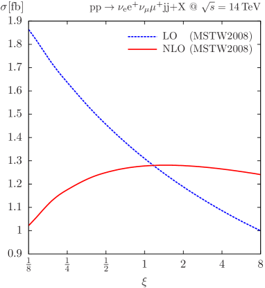
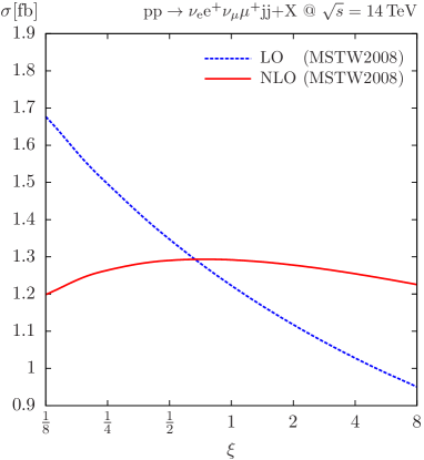
The dependence of the total cross section on the parameter for both scale choices is depicted in Figure 6 for a variation of in the range . In the conventionally chosen range , the scale variation of the LO cross section which only depends on via (as only enters in ) is about , while at NLO it is reduced to about of the total cross section for the FS choice and for the DS choice. For scales down to , the scale dependence for the DS is less pronounced ( of the total cross section at ) than in the case of the FS ( of the total cross section at ). For both scale choices the maximum of the NLO curve is located in the vicinity of (reflecting a small residual scale dependence in this region), so this value is chosen for the subsequent numerical discussions. For , the overall factor, defined as , is
| (4.18) |
respectively, for the two scale choices under consideration.
| 1/8 | 1.6763(2) | 1.6755(2) | 1.6771(2) | 1.198(2) |
|---|---|---|---|---|
| 1/4 | 1.4956(2) | 1.4949(2) | 1.4964(2) | 1.264(1) |
| 1/2 | 1.3467(2) | 1.3461(2) | 1.3474(2) | 1.2903(9) |
| 1 | 1.2224(2) | 1.2218(2) | 1.2230(2) | 1.2917(8) |
| 2 | 1.1173(2) | 1.1168(2) | 1.1179(2) | 1.2778(7) |
| 4 | 1.0275(2) | 1.0270(2) | 1.0280(2) | 1.2544(6) |
| 8 | 0.9499(2) | 0.9494(2) | 0.9504(2) | 1.2253(6) |
The dedicated VBF cuts listed in Section 4.2 prefer - and -channel kinematics, whereas -channel configurations are strongly suppressed by the requirement of final-state jets with large rapidity separation and invariant mass. Moreover, interferences between and channels, showing up in partonic processes with identical final-state (anti-)quarks, are suppressed by the condition that the tagging jets have to be located in opposite—forward and backward—regions of the detector. It can therefore be argued [24] that the -channel and interference contributions can safely be neglected if the VBF cuts are applied. In order to verify this claim, the LO cross section has been evaluated for three different sets of matrix elements; the results (obtained using the DS with selected values of parameter ) can be found in Table 4. Here, stands for the cross section that includes all channels and interferences, while contains the complete - and -channel contributions with interferences but no -channel contributions, and contains only squares of - and -channel contributions but no interferences. One can see that for the cross section within our set of VBF cuts the effect of the – interferences is at the level of , and the contribution of -channel diagrams at the level of . This confirms that can be considered a very good approximation of the full LO cross section. For this reason, the NLO cross section has been evaluated using only - and -channel contributions without interferences between them in order to improve the speed of the calculation. The values of for different values of can be found in the fifth column in Table 4.
4.4 Jet distributions
All distributions shown in this and the following section are evaluated in the numerical setup of Section 4.1, using the kinematic cuts introduced in Section 4.2; the scale choice applied is stated in each case.
Two plots are presented for each observable: the one on the left depicts the LO and NLO predictions, the uncertainty of which is indicated by error bands resulting from variation of the given scale within , while the plot on the right shows the LO and NLO predictions normalized to the LO result at the central scale, i.e. (dotted blue line), and (solid red line). The blue band in this case corresponds to the relative scale uncertainty of the cross section at LO, and the central curve of the red band represents the conventional factor .
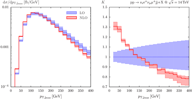
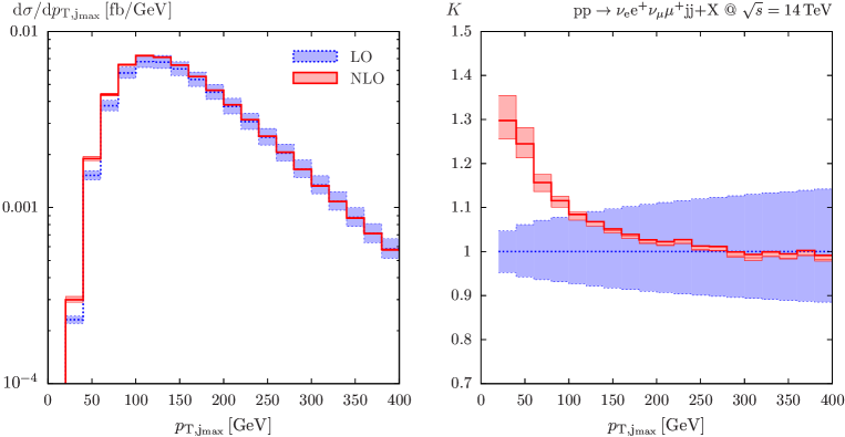
Figure 7 shows the LO and NLO cross sections as functions of the transverse momenta of the harder (in terms of ) of the two tagging jets in the range . Figure 7a displays the dependence for the fixed scale (4.16) and Figure 7b for the dynamic scale (4.17). In both cases, the distribution peaks at , confirming the preference of the high- regions by the VBF tagging jets, while the probability to find a jet at lower values of is slightly larger at NLO than at LO. One can observe that grows noticeably in low- regions for both FS and DS towards the value 1.3, while in the larger- regions it drops to 0.8 in case of the FS (Figure 7a) and remains very close to 1 for the DS (Figure 7b), which is a behaviour that motivated the choice of the DS in the first place.
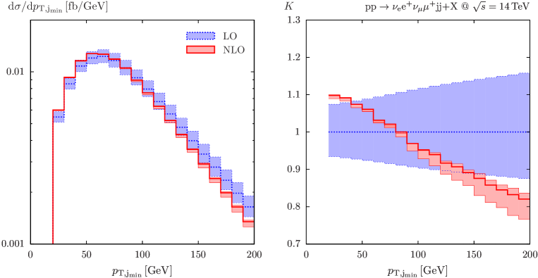
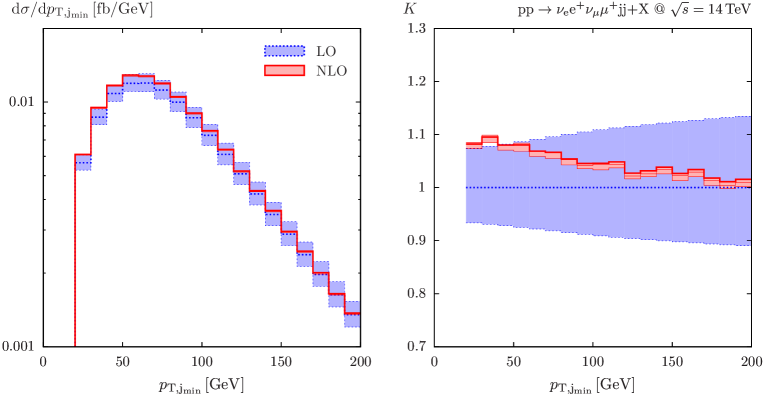
A similar behaviour can be observed with the transverse momentum of the softer tagging jet , as shown in Figure 8. Here, the peak of the distribution is at , indicating that the cut of on the transverse momenta of the tagging jets does not impose any significant reduction to the overall cross section. The variation of is less pronounced than in the case of , while the choice of DS again shows an improvement at reducing contributions from higher-order corrections.
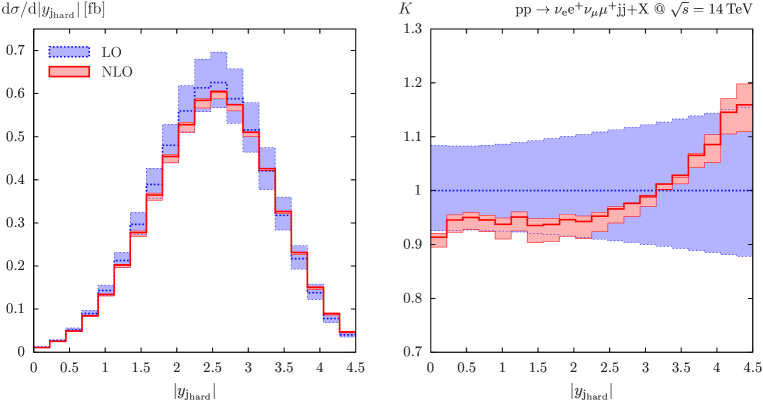
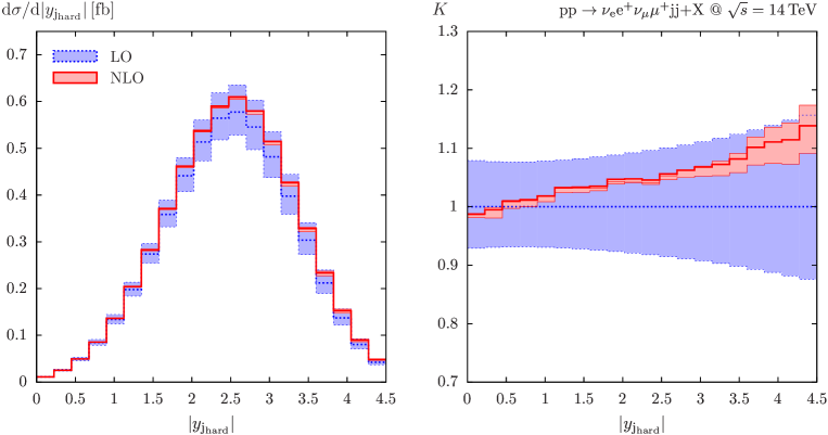
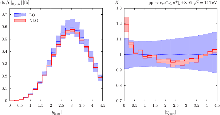
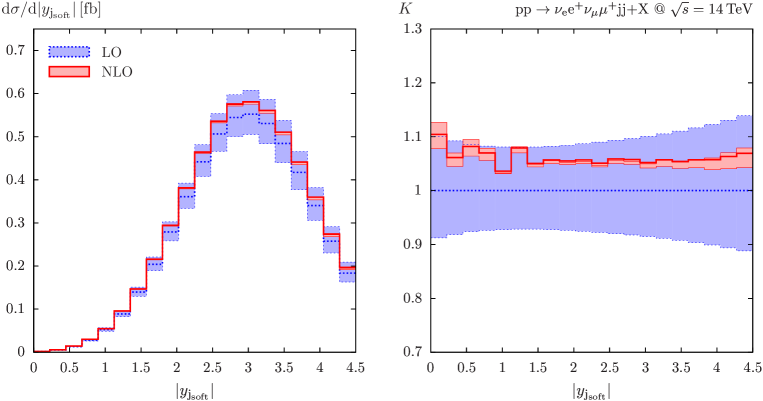
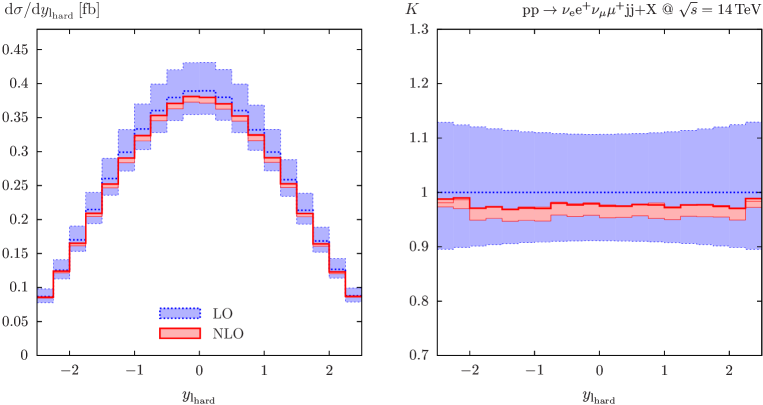
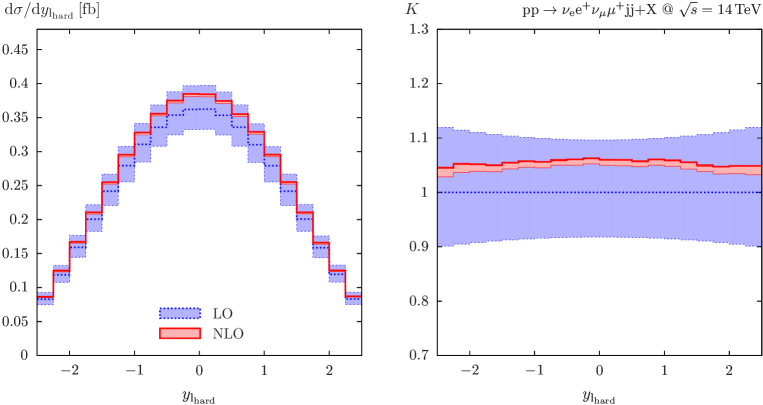
The rapidity of the tagging jets is another distinguishing feature of the VBF processes, as they exhibit very little jet activity in the central region. Absolute rapidity distributions for the harder and softer (in terms of ) tagging jets are shown in Figures 9 and 10, respectively. One can see that the probability to find the harder jet peaks at absolute rapidity of while the softer jet is most likely to be found with absolute rapidity of . This is in sharp contrast to the behaviour for the QCD production mode for , where the jet rapidity peaks at 0, dominating the central rapidity region [8]. This production mode thus can be suppressed dramatically by imposing a cut on the separation of individual jet rapidities (4.11). One can see from Figures 9 and 10 that for both scale choices the rapidity-dependent factor for the hard jet has a tendency to grow for large values of rapidity. This might be attributed to the fact that while only two final-state partons are present at LO, in NLO the tagging jets are selected from up to three partons which might lead to greater dispersion in the rapidity distribution (see discussion in Ref. [24]). As in the case of the transverse-momentum distributions, the DS shows an improvement over the FS in the variation of the factor (Figures 9b and 10b).
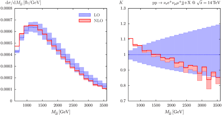
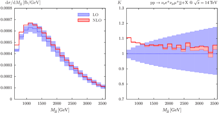
At hadron colliders, QCD processes typically occur at smaller energy scales than EW processes. Due to the back-to-back geometry and large momenta of the tagging jets in VBF, the invariant mass defined in (4.9) can easily exceed , which is typically not the case for any QCD background process, particularly if incoming gluons, which prefer smaller momentum fractions than valence quarks, are involved. For this reason, invariant-mass cuts are applied to distinguish these types of processes. Figure 11 provides the distribution for the invariant mass of the tagging jets for both FS and DS. The peak of the distribution is located at approximately , both at LO and NLO. On a qualitative level, the behaviour of the distributions as well as the factor is in good correspondence to those shown in Ref. [24], in particular for the FS which is set to in both cases. While the DS in Ref. [24] is set to the momentum transfer between the incoming and outgoing partons rather than to , it has a similar effect on the behaviour of the NLO distribution, reducing the scale variation of the factor.
4.5 Leptonic distributions
The decay products of the intermediate gauge bosons in VBF processes can be found almost exclusively in between the tagging jets, in the central region of the detector. This kinematic feature is used to further suppress in particular irreducible background from gluon-mediated contributions to the process , which do not show these characteristics, e.g. by imposing lepton–rapidity cuts like the one in (4.15).
The high leptonic activity in the central region can be well observed in the rapidity distribution of the harder (in terms of ) charged lepton, shown in Figure 12. The distribution shows a preference for the rapidities close to zero, while decreasing quickly as the values approach those of the tagging jets. One can see that for both the FS and the DS the factor remains quite flat. As a similar behaviour can be observed in all presented leptonic distributions, the following distributions are only shown for the DS (4.17).
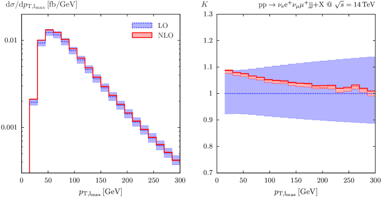
The distribution of the transverse momentum for the harder charged lepton and of the missing corresponding to the vectorial sum of the transverse momenta of the electron neutrino and the muon neutrino from the W decays are shown in Figures 13 and 14, respectively. The factors decrease with increasing transverse momentum and are close to 1 for large .
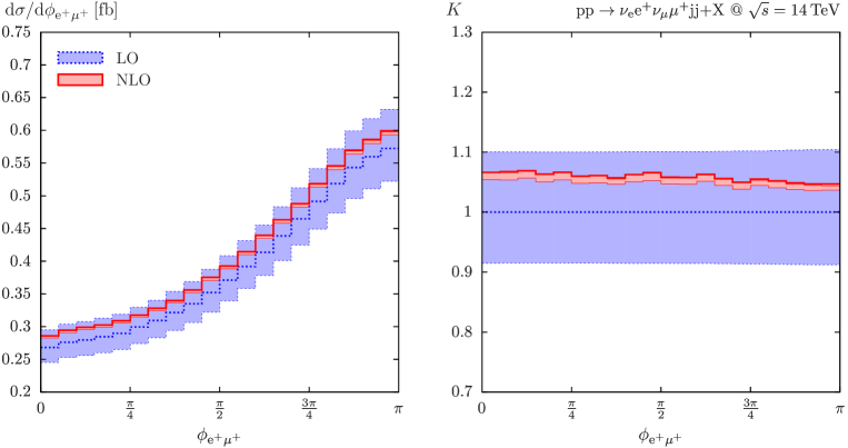
Angular distributions of the decay products of the vector-boson pairs produced in VBF processes are of particular interest to the SM Higgs searches at colliders as the leptons have a tendency to fly in the same direction in case of a Higgs signal [48, 49]. This is due to the fact that a scalar particle decays into a pair of which subsequently decays into charged leptons and neutrinos, with the leptons preferably close to each other due to the left-handed structure of the EW force. This is not the case in the production processes where a SM Higgs decay into both intermediate vector bosons in question is prohibited by the charges. However, a similar situation could arise in the presence of a doubly-charged scalar resonance, which would be produced in the VBF mode and subsequently decay into . The process would then deliver the dominating irreducible background, and the angular distributions of the decay products should be well known to allow for an efficient background suppression. As demonstrated in Figure 15, where the azimuthal angle separating the charged leptons and in the plane transverse to the beam direction is depicted, the final-state leptons are located preferentially in opposite directions in the azimuthal plane. Similarly as with other leptonic observables, the NLO corrections have only a modest effect in this distribution, as exhibited by a flat factor.
5 Conclusions
This article presents a method for evaluating the NLO QCD corrections to the electroweak production mode of processes of the form , associated with vector-boson fusion of an intermediate vector-boson pair, including both resonant contributions where the final-state leptons are produced via vector-boson decay as well as non-resonant ones. The Feynman diagrams are divided into independent building blocks using internal polarization sums and evaluated with the FeynArts + FormCalc package in Mathematica using the Weyl–van der Waerden helicity formalism. The block structure separates the electroweak and QCD sectors of the diagrams, allowing one to apply the QCD corrections only to building blocks involving quark lines while electroweak building blocks are evaluated merely at tree level, improving thus speed of the resulting Fortran code. The phase-space integration is performed by a multichannel Monte Carlo generator implemented in C++ which allows to calculate arbitrary distributions.
The described method is applied to the process , which is interesting in its own right as well as constitutes a background to many collider searches both within and beyond the Standard Model. The numerical analysis is performed using typical vector-boson-fusion cuts chosen to enhance contributions of the vector-boson-fusion kinematics and to suppress QCD background. The impact of the -channel diagrams and interferences between and channels is analyzed at LO and found to be entirely negligible within vector-boson-fusion cuts. The NLO corrections turn out to be around 5% of the LO cross section. The renormalization- and factorization-scale dependence of the cross section at NLO is reduced, amounting to about for the fixed scale and for the dynamical scale , when varying within 1/2 and 2 about , while the LO results change significantly, by , in the same range. Furthermore, a set of kinematical distributions for jets and final-state leptons has been presented, demonstrating the effects of the NLO corrections and the impact of the two scale choices. While the fixed scale results in a strongly decreasing factor in the high-energy tails of the distributions, the factor for the dynamical scale approaches one in these kinematical regions. Using the dynamical scale at leading order provides an approximation to the next-to-leading-order result with an accuracy below about 10% for all considered distributions.
Acknowledgements
L.H. acknowledges the hospitality of the theory groups of PSI and the University of Zurich where most of this work has been done. This work is supported in part by the European Commission through the Marie-Curie Research Training Network HEPTOOLS under contract MRTN-CT-2006-035505 and through the “LHCPhenoNet” Initial Training Network PITN-GA-2010-264564. We are grateful to F. Cascioli, Ph. Maierhöfer, and S. Pozzorini for providing us with OpenLoops matrix elements for LO processes. We thank B. Jäger for helping us to compare our calculation with those of Refs. [24, 8].
References
- [1] M. Dührssen, S. Heinemeyer, H. Logan, D. Rainwater, G. Weiglein, et al., Extracting Higgs boson couplings from CERN LHC data, Phys.Rev. D70 (2004) 113009, [hep-ph/0406323].
- [2] A. Belyaev and L. Reina, , : Toward a model independent determination of the Higgs boson couplings at the LHC, JHEP 0208 (2002) 041, [hep-ph/0205270].
- [3] V. Hankele, G. Klämke, D. Zeppenfeld, and T. Figy, Anomalous Higgs boson couplings in vector boson fusion at the CERN LHC, Phys.Rev. D74 (2006) 095001, [hep-ph/0609075].
- [4] K. Hagiwara, Q. Li, and K. Mawatari, Jet angular correlation in vector-boson fusion processes at hadron colliders, JHEP 0907 (2009) 101, [arXiv:0905.4314].
- [5] J. Bagger, V. D. Barger, K.-m. Cheung, J. F. Gunion, T. Han, et al., CERN LHC analysis of the strongly interacting W W system: Gold plated modes, Phys.Rev. D52 (1995) 3878–3889, [hep-ph/9504426].
- [6] A. Ballestrero, D. B. Franzosi, and E. Maina, Vector-Vector scattering at the LHC with two charged leptons and two neutrinos in the final state, JHEP 1106 (2011) 013, [arXiv:1011.1514].
- [7] D. L. Rainwater, R. Szalapski, and D. Zeppenfeld, Probing color singlet exchange in + two jet events at the CERN LHC, Phys.Rev. D54 (1996) 6680–6689, [hep-ph/9605444].
- [8] B. Jäger and G. Zanderighi, NLO corrections to electroweak and QCD production of plus two jets in the POWHEG BOX, JHEP 1111 (2011) 055, [arXiv:1108.0864].
- [9] H. Dreiner, S. Grab, M. Krämer, and M. Trenkel, Supersymmetric NLO QCD corrections to resonant slepton production and signals at the Tevatron and the CERN LHC, Phys.Rev. D75 (2007) 035003, [hep-ph/0611195].
- [10] T. Han, I. Lewis, and T. McElmurry, QCD Corrections to Scalar Diquark Production at Hadron Colliders, JHEP 1001 (2010) 123, [arXiv:0909.2666].
- [11] J. Maalampi and N. Romanenko, Single production of doubly charged Higgs bosons at hadron colliders, Phys.Lett. B532 (2002) 202–208, [hep-ph/0201196].
- [12] A. Kulesza and W. J. Stirling, Like sign boson production at the LHC as a probe of double parton scattering, Phys.Lett. B475 (2000) 168–175, [hep-ph/9912232].
- [13] E. Maina, Multiple Parton Interactions in and production at the LHC, JHEP 0909 (2009) 081, [arXiv:0909.1586].
- [14] J. R. Gaunt, C.-H. Kom, A. Kulesza, and W. J. Stirling, Same-sign W pair production as a probe of double parton scattering at the LHC, Eur.Phys.J. C69 (2010) 53–65, [arXiv:1003.3953].
- [15] T. Melia, K. Melnikov, R. Rontsch, and G. Zanderighi, Next-to-leading order QCD predictions for production at the LHC, JHEP 1012 (2010) 053, [arXiv:1007.5313].
- [16] T. Melia, K. Melnikov, R. Rontsch, and G. Zanderighi, NLO QCD corrections for pair production in association with two jets at hadron colliders, Phys.Rev. D83 (2011) 114043, [arXiv:1104.2327].
- [17] N. Greiner, G. Heinrich, P. Mastrolia, G. Ossola, T. Reiter, et al., NLO QCD corrections to the production of plus two jets at the LHC, Phys.Lett. B713 (2012) 277–283, [arXiv:1202.6004].
- [18] T. Melia, P. Nason, R. Rontsch, and G. Zanderighi, plus dijet production in the POWHEGBOX, Eur.Phys.J. C71 (2011) 1670, [arXiv:1102.4846].
- [19] P. Nason, A New method for combining NLO QCD with shower Monte Carlo algorithms, JHEP 0411 (2004) 040, [hep-ph/0409146].
- [20] S. Frixione, P. Nason, and C. Oleari, Matching NLO QCD computations with Parton Shower simulations: the POWHEG method, JHEP 0711 (2007) 070, [arXiv:0709.2092].
- [21] B. Jäger, C. Oleari, and D. Zeppenfeld, Next-to-leading order QCD corrections to production via vector-boson fusion, JHEP 07 (2006) 015, [hep-ph/0603177].
- [22] B. Jäger, C. Oleari, and D. Zeppenfeld, Next-to-leading order QCD corrections to Z boson pair production via vector-boson fusion, Phys. Rev. D73 (2006) 113006, [hep-ph/0604200].
- [23] G. Bozzi, B. Jäger, C. Oleari, and D. Zeppenfeld, Next-to-leading order QCD corrections to and production via vector-boson fusion, Phys. Rev. D75 (2007) 073004, [hep-ph/0701105].
- [24] B. Jäger, C. Oleari, and D. Zeppenfeld, Next-to-leading order QCD corrections to and production via weak-boson fusion, Phys. Rev. D80 (2009) 034022, [arXiv:0907.0580].
- [25] L. Hošeková, “NLO QCD corrections to the production of two lepton pairs via vector-boson fusion at the LHC.” doctoral thesis, Zurich University, 2012.
- [26] M. Ciccolini, A. Denner, and S. Dittmaier, Electroweak and QCD corrections to Higgs production via vector-boson fusion at the LHC, Phys.Rev. D77 (2008) 013002, [arXiv:0710.4749].
- [27] T. Hahn, FormCalc 6, PoS ACAT08 (2008) 121, [arXiv:0901.1528].
- [28] S. Dittmaier, Weyl-van der Waerden formalism for helicity amplitudes of massive particles, Phys.Rev. D59 (1998) 016007, [hep-ph/9805445].
- [29] S. Catani and M. H. Seymour, A general algorithm for calculating jet cross sections in NLO QCD, Nucl. Phys. B485 (1997) 291–419, [hep-ph/9605323].
- [30] A. Denner and S. Dittmaier, Reduction of one-loop tensor 5-point integrals, Nucl. Phys. B658 (2003) 175–202, [hep-ph/0212259].
- [31] A. Denner and S. Dittmaier, Reduction schemes for one-loop tensor integrals, Nucl. Phys. B734 (2006) 62–115, [hep-ph/0509141].
- [32] A. Denner, U. Nierste, and R. Scharf, A Compact expression for the scalar one loop four point function, Nucl. Phys. B367 (1991) 637–656.
- [33] W. Beenakker and A. Denner, Infrared Divergent Scalar Box Integrals with Applications in the Electroweak Standard Model, Nucl. Phys. B338 (1990) 349–370.
- [34] A. Denner and S. Dittmaier, Scalar one-loop 4-point integrals, Nucl.Phys. B844 (2011) 199–242, [arXiv:1005.2076].
- [35] A. Denner, S. Dittmaier, and L. Hofer, “COLLIER, Complex One-Loop Library In Extended Regularizations.” in preparation.
- [36] A. Denner, S. Dittmaier, M. Roth, and D. Wackeroth, Predictions for all processes 4 fermions , Nucl.Phys. B560 (1999) 33–65, [hep-ph/9904472].
- [37] A. Denner, S. Dittmaier, M. Roth, and L. Wieders, Electroweak corrections to charged-current 4 fermion processes: Technical details and further results, Nucl.Phys. B724 (2005) 247–294, [hep-ph/0505042].
- [38] A. Denner and S. Dittmaier, The complex-mass scheme for perturbative calculations with unstable particles, Nucl.Phys.Proc.Suppl. 160 (2006) 22–26, [hep-ph/0605312].
- [39] J. Alwall, P. Demin, S. de Visscher, R. Frederix, M. Herquet, et al., MadGraph/MadEvent v4: The New Web Generation, JHEP 0709 (2007) 028, [0706.2334].
- [40] F. Cascioli, P. Maierhofer, and S. Pozzorini, Scattering Amplitudes with Open Loops, Phys.Rev.Lett. 108 (2012) 111601, [arXiv:1111.5206].
- [41] A. Denner, S. Dittmaier, S. Kallweit, and S. Pozzorini, NLO QCD corrections to off-shell top-antitop production with leptonic decays at hadron colliders, arXiv:1207.5018.
- [42] Particle Data Group Collaboration, J. Beringer et al., Review of Particle Physics (RPP), Phys.Rev. D86 (2012) 010001.
- [43] S. Dittmaier and M. Krämer, Electroweak radiative corrections to W boson production at hadron colliders, Phys.Rev. D65 (2002) 073007, [hep-ph/0109062].
- [44] A. Martin, W. Stirling, R. Thorne, and G. Watt, Parton distributions for the LHC, Eur.Phys.J. C63 (2009) 189–285, [arXiv:0901.0002].
- [45] S. Dittmaier, C. Mariotti, G. Passarino, R. Tanaka, et al., Handbook of LHC Higgs Cross Sections: 2. Differential Distributions, arXiv:1201.3084.
- [46] S. Catani, Y. L. Dokshitzer, and B. Webber, The perpendicular clustering algorithm for jets in deep inelastic scattering and hadron collisions, Phys.Lett. B285 (1992) 291–299.
- [47] G. C. Blazey, J. R. Dittmann, S. D. Ellis, V. D. Elvira, K. Frame, et al., Run II jet physics, hep-ex/0005012.
- [48] M. Dittmar and H. K. Dreiner, as the dominant SM Higgs search mode at the LHC for GeV–GeV, hep-ph/9703401.
- [49] D. L. Rainwater and D. Zeppenfeld, Observing in weak boson fusion with dual forward jet tagging at the CERN LHC, Phys.Rev. D60 (1999) 113004, [hep-ph/9906218].