Efficient simulation of infinite tree tensor network states on the Bethe lattice

Abstract

We show that the simple update approach proposed by Jiang et al [H.C. Jiang, Z.Y. Weng, and T. Xiang, Phys. Rev. Lett. 101, 090603 (2008)] is an efficient and accurate method for determining the infinite tree tensor network states on the Bethe lattice. Ground state properties of the quantum transverse Ising model and the Heisenberg XXZ model on the Bethe lattice are studied. The transverse Ising model is found to undergo a second-order quantum phase transition with a diverging magnetic susceptibility but a finite correlation length which is upper-bounded by $1/\ln(q-1)$ even at the transition point ($q$ is the coordinate number of the Bethe lattice). An intuitive explanation on this peculiar “critical” phenomenon is given. The XXZ model on the Bethe lattice undergoes a first-order quantum phase transition at the isotropic point. Furthermore, the simple update scheme is found to be related with the Bethe approximation. Finally, by applying the simple update to various tree tensor clusters, we can obtain rather nice and scalable approximations for two-dimensional lattices.

I introduction

The investigation of quantum lattice models is one of the central themes in modern condensed matter physics. A crucial step is to develop novel numerical methods to efficiently simulate the interesting and complex phenomena of quantum many-body systems. In particular, the tensor network states and the related renormalization group methods, including the tree tensor network state (TTN),Shi ; Tagliacozzo ; Murg the multi-scale entanglement renormalization ansatz,MERA the projected entangled pair state,Verstraete the tensor renormalization group (TRG),Levin ; Xiang ; Gu and the second renormalization group (SRG),Xie ; Zhao are now under rapid development. These methods provide promising numerical tools for studying strongly correlated systems, especially for the frustrated magnetic systems and fermion models, and can be regarded as an extension of the fruitful density matrix renormalization group (DMRG)White in two or higher dimensions.

In the study of the tensor network methods, one needs to first determine the tensor network wavefunction for the ground state. In Refs. [Xiang, ; Zhao, ], a simple update scheme is proposed to determine the ground state tensor network wavefunction in two dimensions. This scheme is efficient and robust. It proceeds in three steps: (1) apply the imaginary time projection operators simultaneously on bonds of the same type, for example the $x$ directional bonds in Fig. 1a, and enlarge the bond dimension; (2) construct a local evolving block matrix and simulate the environment contribution by the diagonal matrices on the external bonds [$\lambda_{y}$ and $\gamma_{z}$ in Fig. 1b]; (3) decompose the evolving block matrix by singular value decomposition (SVD) and decimate the vector space of the enlarged geometric bond according to the singular values in the updated diagonal matrix $\theta^{\prime}_{x}$. This technique has been combined with the TRG/SRG to evaluate the ground state properties of two-dimensional (2D) Heisenberg models.Zhao ; Gu ; Chen ; Li ; Zhao2 It is an accurate numerical method for evaluating local physical quantities, but it is less accurate in evaluating the long-range correlation functions.Zhao This is the major drawback of this simple update scheme. It results from a mean-field approximation for the environment tensor. A way to go beyond this approximation is to enlarge the size of the cluster that is used for evaluating the environment tensor. This, as shown by Wang and VerstraeteWang , can indeed improve the accuracy for the long range correlation function.

In this work, we apply the simple update scheme to infinite TTN (iTTN) states on the Bethe lattice. We will show that this is a quasi-canonical approach for treating an iTTN. Here by the word “quasi-canonical” we mean that with increasing the number of iteration steps and decreasing the Trotter error, the tree tensor network state obtained by the simple update scheme would become asymptotically canonical [i.e. the tensors satisfy certain canonical orthonormality conditions, see Eqs. (3) below]. Thus the simple update scheme provides an accurate and efficient approach for evaluating the ground state wavefunction on the Bethe lattice.

The Bethe lattice, as shown in Fig. 1a, has a self-similar structure with an infinite Hausdorff dimension. The size of the lattice is infinite, hence the boundary effects do not need to be explicitly considered. The Bethe lattice was first used in the study of classical statistical mechanics.Bethe ; Plischke ; Baxter It has attracted broader interest since a number of chemical compounds with the Bethe lattice structures, such as the dendrimers,Delgado have been synthesized in the laboratory.Astruc

A finite Bethe lattice is called a Cayley tree. Soon after White’s invention of DMRG,White the DMRG algorithm for the quantum lattice models defined on the Cayley tree was proposed. Otsuka ; Friedman Based on the DMRG calculation of local physical quantities in the central part of the Cayley tree, OtsukaOtsuka claimed that the anisotropic S=1/2 Heisenberg model (i.e. the XXZ model) on the Bethe lattice should exhibit a first-order phase transition at the isotropic point. Later FriedmanFriedman proposed an improved DMRG scheme and evaluated the spin-spin correlations in the ground state. Based on the DMRG result, he suggested that long-range magnetic order might exist at the isotropic Heisenberg point. Recently, Kumar et al. calculated the magnetization with a further improved DMRG algorithm, Kumar and showed that such long-range magnetic order does exist at that point.

The above DMRG calculations were done on the Cayley tree lattice, not on the true infinite Bethe lattice. Furthermore, it should be pointed out that the boundary effect is very strong on a finite Cayley tree since more than one-half of the total sites reside on the lattice edge. This may strongly affect the properties of the system. In some cases, the results obtained on a Cayley tree lattice can be completely different from those for the corresponding Bethe lattice. For example, the classical Ising model shows a phase transition on the Bethe lattice, but not on the Cayley tree lattice.Ostilli

To unambiguously resolve the above problems, it is necessary to calculate the spin models directly on the Bethe lattice. The recent development of the TTN algorithms Shi ; Tagliacozzo ; Murg has indeed made this feasible.Nagaj ; Nagy In particular, Nagaj et al in Ref. Nagaj, extended the infinite time evolving-block decimationVidal technique to the Bethe lattice and determined the ground state wavefunction by imaginary time evolution. For the transverse Ising model on the Bethe lattice, it was found that a second-order quantum phase transition exists at a critical transverse field. An interesting result revealed in this calculation is that even at the second-order critical point, the correlation length remains finite. For the Bethe lattice with coordination $q=3$, the correlation length is shown to be less than $1/\ln 2$. However, in the calculation Nagaj et al used a three-site projection operator to simultaneously evolve the two equivalent incoming legs of the tensors, the computational cost is thus very high. The computational time scales as O($D^{8}$) with $D$ the tensor dimension, which limits the value of $D$ that can be handled to $D\leq 8$.

Recently, NagyNagy proposed a different algorithm to reduce the computational cost by making use of the $C_{3}$ rotational symmetry of $q=3$ Bethe lattice. This algorithm reduces the computational cost to O($D^{4}$) hence greatly improves the efficiency. It can be used for studying the spin-1/2 quantum lattice models. However, the application of this method is restricted to the translation invariant spin-1/2 system.

Figure 1: (Color online) (a) The $q=3$ Bethe lattice. Every site has 3 nearest neighbors, and the three bonds are labeled according to their directions as $x$, $y$, and $z$, respectively. (b) The two-site cluster used in the single-bond projection of the simple update scheme. The diagonal matrices $\lambda_{y}$ and $\gamma_{z}$ on the dangling bonds should be included in the projection to mimic the entanglement renormalization of the environment to this two-site system. (c) A minimum cluster that is used in the Bethe approximation. It consists of one A tensor and three nearest-neighbor B tensors (or vice versa).

As will be shown below, the simple update scheme is very efficient. Its computational costs scale as O($D^{4}$), similar as for the algorithm proposed by NagyNagy . But it is much more flexible. It can be applied to treat arbitrary TTN states, with or without translation invariance. Here we studied two spin models defined on the Bethe lattice. One is the transverse Ising model and the other is the antiferromagnetic XXZ Heisenberg model. The quantum phase transitions and the ground state phase diagrams of these models are studied.

The rest of the paper is arranged as follows. An introduction to the simple update scheme and its relationship with the Bethe approximation is presented in Sec. II. The study of the quantum phase transitions of transverse Ising and XXZ Heisenberg models are presented in Secs. III and IV, respectively. In Sec. V, the present scheme is generalized to larger tree tensor clusters, in order to provide more accurate approximations for 2D lattices. Finally, Sec VI is devoted to a summary.

II The canonical form and the simple update scheme

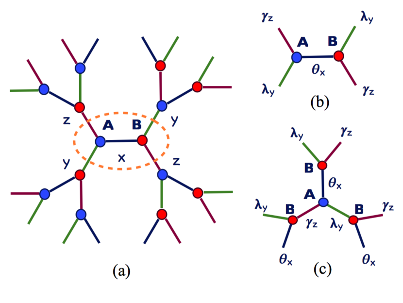
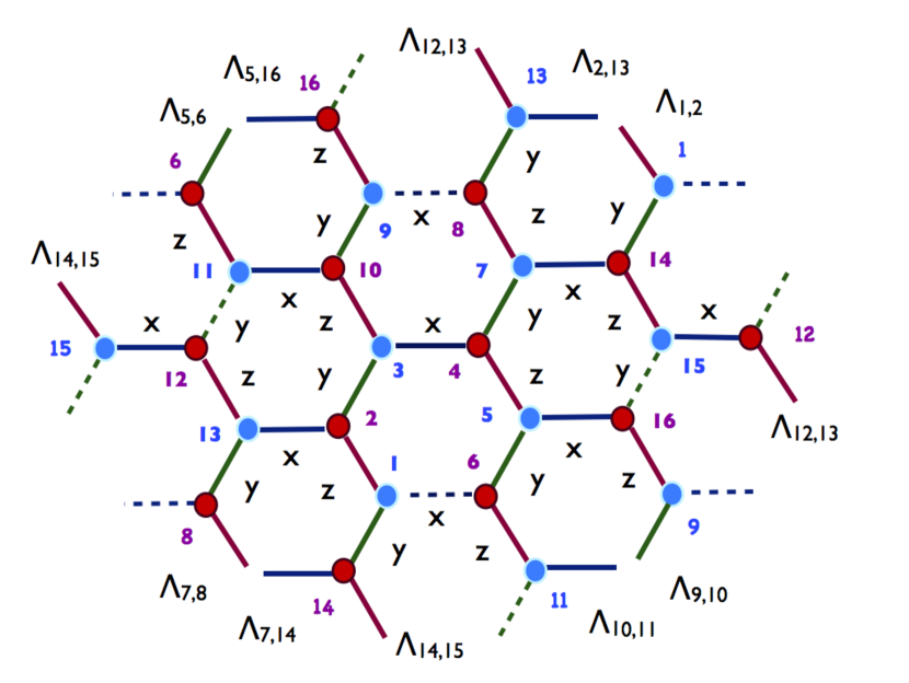
The iTTN state on the Bethe lattice comprises 4-indexed tensors $A_{x,y,z}^{m}$ and $B_{x,y,z}^{m}$ defined on the vertices, and the diagonal matrices $\theta$, $\lambda$, $\gamma$ defined on the bonds along the $x$, $y$, and $z$ directions as shown in Fig. 1a, respectively. The bond indices represent the quantum numbers of the virtual basis states. The physical index $m$ runs over the $d$ basis states of the local Hilbert space at each lattice site. The diagonal matrices store the entanglement information, and play an important role in the simple update scheme.

In order to determine the ground state wavefunction, the imaginary time evolving operators $U(\tau)=\exp{(-\tau h_{i,j})}$ are applied to the iTTN iteratively. At each step, the dimension of the evolved bond is increased by a factor of $d^{2}$. Thus the tensor dimensions will proliferate exponentially with the increasing number of projection steps. In order to sustain the projections until the iTTN converges to the true ground state wavefunction, one needs to truncate the bond dimension after each projection step. This needs a proper consideration of the renormalization effect of the environment tensor.

An accurate and full determination of the environment tensor is computationally costly. This limits generally the tensor dimension $D$ that can be handled to a rather small value, say $D\leq 6$. The simple update schemeXiang ; Xie ; Zhao , on the other hand, takes the product of the dangling bond matrices as a mean field approximation to the environment tensor. It converts the complicated global optimization problem into a local one, and hence greatly simplifies the calculation. On the regular 2D lattice, the bond matrix is an approximate measure of the entanglement between the system and environment tensors. However, as will be shown later, the square of the diagonal bond matrix on the Bethe lattice is the eigenvalue of the reduced density matrix if the iTTN is canonicalized, i.e., if the tensors in the network are always kept in canonical form by some transformations. Thus the simple update scheme is an accurate treatment for the renormalization of the iTTN on the Bethe lattice.

The simple update scheme is also closely related to the famous Bethe approximation.Bethe ; Plischke ; Baxter To understand this, we show in Fig. 1c a 4-site cluster, which contains one A tensor and three B tensors. In the simple update calculation, the two local tensors, A and B, and the three inner bond matrices ($\theta_{x}$, $\lambda_{y}$, $\gamma_{z}$) should be evaluated and updated iteratively. After each single projection step on the inner bonds, to keep the scheme self-consistent, one should also update all the dangling bonds of the cluster, by replacing the bond matrices with the corresponding ones on the inner bonds.

This cluster structure and the self-consistent scheme is in fact the Bethe approximation that was first proposed by Bethe in 1930’s, in the context of statistical mechanics.Bethe The key idea is to treat the correlations between the central spin and its nearest neighbors in the cluster exactly, and to use an effective mean field to approximate the interactions between the cluster and the rest lattice spins. By solving this simple cluster problem, and assuming that all the spins in the cluster have exactly the same local magnetization, one can determine the spontaneous magnetization self-consistently. For the quantum cases, the six diagonal matrices on the dangling bonds of the cluster are taken as the mean fields acting on the inner block. The self-consistent condition requires that the matrices $\theta$, $\lambda$, and $\gamma$ on dangling bonds are equal to the corresponding matrices on the inner bonds between A and B tensors (see Fig. 1c).

Figure 2: (Color online) One iteration step in the simple update scheme: (a) A and B tensors are connected by the bond $x$, which will be involved in the following projection steps. There are diagonal matrices on the dangling bonds ($y$ and $z$ bonds) of A and B tensors. (b) Absorb the four dangling matrices into A and B, and define the block matrix $M_{a(b)}$. Then take the QR decomposition for $M_{a(b)}$, obtaining $Q_{a(b)}$ and $R_{a(b)}$ matrices. (c) Project $U(\tau)$ onto the bond by contractions, and obtain the block matrix $G$ [see Eq. (7)]. (d) Take singular value decomposition of $G$ to find the unitary matrices $U$ and $V^{T}$, and the new diagonal matrix $\theta^{\prime}$. (e) Truncate the $x$-bond dimension to $D$ according to the diagonal values of $\theta^{\prime}$. Merge $U$ ($V^{T}$), $\gamma_{y}^{-1}$, and $\lambda_{z}^{-1}$ together into $Q_{a(b)}$, finally we arrive at the updated $A^{\prime}(B^{\prime})$ tensors.

A tensor network state contains redundant gauge degrees of freedom on each bond. It is invariant if one inserts a product of two reciprocal matrices on a bond and absorbs separately each of them to a local tensor at the two ends of the bond. This gauge invariance of a tensor network state can be used to simplify the calculation of local tensors, especially for the iTTN states on the Bethe lattice, where a special gauge, called canonical form, can be introduced.

To be specific, the local tensors of canonical iTTN states satisfy the following orthonormality conditions

$$\sum_{m}\sum_{x,y}\theta_{x}^{2}\lambda_{y}^{2}(T^{m}_{x,y,z^{\prime}})^{*}T^{m}_{x,y,z} = \delta_{z^{\prime},z},$$ (1)

$$\sum_{m}\sum_{y,z}\lambda_{y}^{2}\gamma_{z}^{2}(T^{m}_{x^{\prime},y,z})^{*}T^{m}_{x,y,z} = \delta_{x^{\prime},x},$$ (2)

$$\sum_{m}\sum_{z,x}\gamma_{z}^{2}\theta_{x}^{2}(T^{m}_{x,y^{\prime},z})^{*}T^{m}_{x,y,z} = \delta_{y^{\prime},y},$$ (3)

where T represents the A or B tensor. If we cut an arbitrary bond to divide the Bethe lattice into two parts, denoted as a system and an environment subblock, one can then define the reduced density matrix of the system block by integrating out all the degrees of freedom of the environment block. For the tensors that satisfy Eqs. (1-3), the square of the diagonal bond matrices are the eigenvalues, and the renormalized bond bases are the eigenvectors of the corresponding reduced density matrix, which are orthonormal to each other. Thus, in terms of the Schmidt decomposition, the square of the diagonal matrix elements represent the probability amplitudes of the corresponding eigenvectors appearing in the wavefunction.

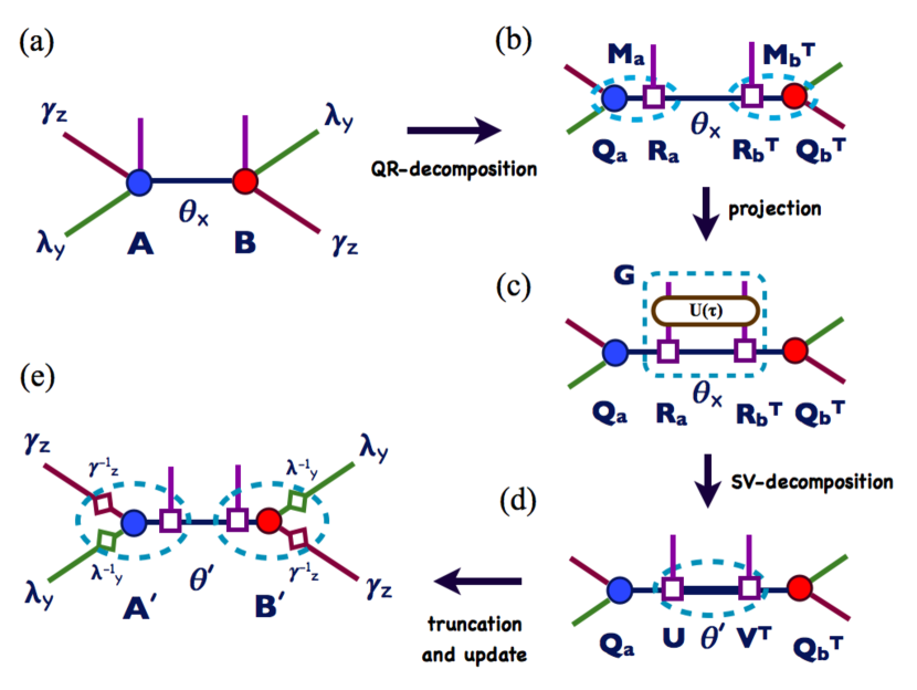
The existence of this simple canonical form of the iTTN, i.e. Eqs. (1-3), is very useful in the calculations. First, the diagonal bond matrix describes the entanglement spectrum between the system and environment subblocks. Thus to select the virtual bond basis states according to the values of these diagonal matrix elements provides an optimal scheme to truncate the bond dimension. Second, the contribution of the environment tensors can be faithfully represented by the 4 diagonal matrices on the dangling bonds surrounding the central bond under projection (see Fig. 2a). It means that the imaginary time evolution on each bond can be done rigorously and locally. Furthermore, we can also evaluate the expectation value of a local operator simply by contracting a small cluster comprising those tensors and bond matrices on which the operator acts. This significantly reduces the computational cost.

Bearing in mind the benefits of the canonical iTTN states, one can perform explicitly the canonical transformations during the projection processes. However, to further save computational costs, in practical calculations we choose to carry out the imaginary time evolution just using the simple update scheme, and gradually reduce the Trotter step $\tau$, which would bring the iTTN states into its canonical form step by step. This scheme works because the diagonal bond matrix provides an approximate measure for the entanglement between the two sides of the bond and can be used to substitute approximately the environment tensor. Therefore, it can stabilize the algorithm of the imaginary time evolution, provided that the Trotter step $\tau$ is small enough so that the bond projection operator $U(r)$ is nearly unitary.Vidal This near unitary evolution can modify the wavefunction and reshape it in order to satisfy the canonical conditions. The simple update scheme hence provides a quasi-canonical evolution of the iTTN state, which will finally converge to the ground state and become canonical in the limit $\tau\rightarrow 0$. In practical calculations, the Trotter step $\tau$ is gradually decreased from $10^{-1}$ to $10^{-4}$, and the total number of projections steps varies from 20000 to 200000.

Now let us consider how to implement the simple update scheme efficiently. A simple approach is to do directly the singular value decomposition the evolving block tensor, which is a matrix of $D^{2}\times D^{2}$. The computational cost for doing this singular value decomposition is high, since it scales as $O(D^{6})$. This cost can in fact be reduced to $O(D^{4})$ if we carry out this singular value decomposition in the following steps (again, projection on $x$ bond is taken as an example):

(1) Define the following two $D^{2}\times Dd$ block matrices (Fig. 2b)

$$(M_{a})_{y,z;x,m} = \lambda_{y}\gamma_{z}A_{xyz}^{m},$$ (4)

$$(M_{b})_{y,z;x,m} = \lambda_{y}\gamma_{z}B_{xyz}^{m},$$ (5)

by absorbing the diagonal matrices $\lambda_{y}$ and $\gamma_{z}$ into the tensors A and B, and calculate their QR decomposition

$$(M_{\alpha})_{y,z;x,m}=\sum_{k}Q^{\alpha}_{y,z;k}R^{\alpha}_{k;m,x},$$ (6)

where $\alpha=a$ or $b$. $Q^{\alpha}$ is a $D^{2}\times Dd$ column orthonormal matrix. $R^{\alpha}$ is a $Dd\times Dd$ upper diagonal matrix.

(2) Apply the bond projection operator $U(\tau)$ to the system and define the gate matrix (Fig. 2c)

$$G_{m_{1}k_{1};m_{2}k_{2}}=\sum_{x,m_{1}^{\prime},m^{\prime}_{2}}\langle m_{1}m_{2}|U(\tau)|m_{1}^{\prime}m^{\prime}_{2}\rangle R^{a}_{k_{1};m_{1}^{\prime}x}\theta_{x}R^{b}_{k_{2};m_{2}^{\prime}x}$$ (7)

(3) Take the singular value decomposition for this matrix (Fig. 2d),

$$G_{m_{1}k_{1};m_{2}k_{2}}=U_{m_{1}k_{1};l}\theta^{\prime}_{l}V_{m_{2}k_{2};l},$$ (8)

where $U$ and $V$ are two $Dd\times Dd$ unitary matrices, and $\theta^{\prime}$ is a semi-positive defined matrix.

(4) Truncate the inner bond dimension by keeping the largest $D$ matrix elements of $\theta^{\prime}$, and update the local tensors by the formula (Fig. 2e)

$${A^{\prime}}^{m}_{xyz} = \sum_{k}\lambda_{y}^{-1}\gamma_{z}^{-1}Q^{a}_{y,z;k}U_{m,k;x},$$ (9)

$${B^{\prime}}^{m}_{xyz} = \sum_{k}\lambda_{y}^{-1}\gamma_{z}^{-1}Q^{b}_{y,z;k}V_{m,k;x}.$$ (10)

Combining this efficient simple update scheme and the local determination of physical observables using the canonical form, we can keep the computational cost in a low level. In practice, this allows us to keep a relative large bond dimension.

Figure 3: (Color online) (a) The longitudinal and transverse magnetizations $m_{z}$ and $m_{x}$ versus the transverse fields $h_{x}$. The transverse magnetization $m_{x}$ increases monotonously with $h_{x}$, while the longitudinal magnetization $m_{z}$ decreases and vanishes at the transition point. (b) The second-order derivative of the ground state energy per site $e$ with respect to $h_{x}$, $d^{2}e/dh_{x}^{2}$, obtained by taking the first-order derivative of $m_{x}$, $dm_{x}/dh_{x}$.

III The transverse Ising model

The transverse Ising model is defined by the Hamiltonian

$$H_{\rm{TI}}=-\sum_{<i,j>}JS_{i}^{z}S_{j}^{z}-\sum_{i}h_{x}S_{i}^{x}-\sum_{i}h_{z}S_{i}^{z},$$ (11)

where the spin-spin exchange constant $J$ is set as the energy scale ($J=1$, ferromagnetic coupling). The second term represents the transverse-field along $S^{x}$ direction, and the last term is the longitudinal-field along $S^{z}$ direction.

Figure 4: (Color online) (a) The entanglement entropy $S_{\rm{E}}$ of the ground state for the transverse Ising model. The cusp at $h_{c}\simeq 1.115$ corresponds to the second-order phase transition point. (b) The correlation length $\xi$ of the ground state, which also shows a cusp at the transition point.

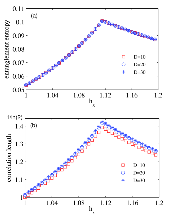
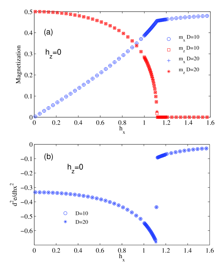
Figure 3a shows the longitudinal and transverse magnetizations, $m_{z}=\langle S_{z}\rangle$ and $m_{x}=\langle S_{x}\rangle$, as a function of the transverse field $h_{x}$. A continuous order-disorder phase transition is found at $h_{c}$. For $h_{x}<h_{c}$, the ground states undergo a spontaneous $Z_{2}$ symmetry breaking with a finite longitudinal magnetization $m_{z}$, which decreases with increasing $h_{x}$ and vanishes at the critical field. By utilizing the Hellmann-Feynman theorem, the second-order derivative of the ground state energy can be calculated by $d^{2}e/dh_{x}^{2}=-dm_{x}/dh_{x}$. As shown in Fig. 3b, $d^{2}e/dh_{x}^{2}$ exhibits a discontinuity at $h_{c}$, indicating that $h_{c}$ is a second-order phase transition point. The critical field is found to be $h_{c}\simeq 1.115$, in agreement with previous calculations.Nagaj ; Nagy It is also close to the critical field $h_{c}=1.06625(2)$ for the transverse Ising model on the honeycomb lattice.Deng

Figure 5: (Color online) The field dependence of the longitudinal susceptibility $\chi^{z}$. It shows a divergent peak at the transition point $h_{c}\simeq 1.116$. The susceptibility is calculated by $\chi^{z}=[m_{z}(h_{z})-m(0)]/\delta h$ with $h_{z}=10^{-4}$.

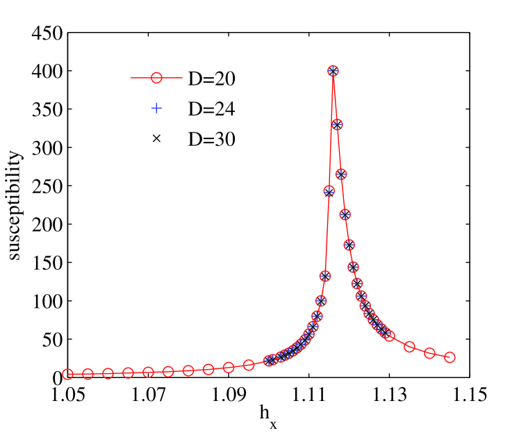
Figure 4 shows the bipartite entanglement entropy $S_{\rm{E}}$

$$S_{\rm{E}}=-\rm{Tr}[\Lambda^{2}\log_{2}(\Lambda^{2})],$$ (12)

and the correlation length $\xi$ for the ground state. In Eq. (12), $\Lambda$ = $\theta$, $\lambda$ or $\gamma$ is a diagonal matrix that satisfies the canonical condition. $S_{\rm{E}}$ shown in Fig. 4a is obtained by taking the average over the three bonds.

The correlation length $\xi$ is evaluated from the ratio of the the largest ($a_{0}$) and the second largest eigenvalue ($a_{1}$) of the transfer-matrix for the iTTN state,

$$\xi=1/\ln{\frac{a_{0}}{a_{1}}}\;.$$ (13)

For the $q=3$ Bethe lattice, there are six kinds of transfer-matrices, depending on the site and the bond direction. For example the transfer matrix along the $yz$-direction is defined by (for A sublattice site)

$$T^{a}_{y,z;y^{\prime},z^{\prime}}=\sum_{m,x}\sqrt{\lambda_{y}\gamma_{z}}(A^{m}_{x,y,z})^{*}\theta^{2}_{x}A^{m}_{x,y^{\prime},z^{\prime}}\sqrt{\lambda_{y^{\prime}}\gamma_{z^{\prime}}}.$$ (14)

The other five transfer matrices including $T^{b}_{y,z;y^{\prime},z^{\prime}}$, $T^{a,b}_{z,x;z^{\prime},x^{\prime}}$, and $T^{a,b}_{x,y;x^{\prime},y^{\prime}}$ can be similarly defined. The results of the correlation length shown in Fig. 4b are evaluated from the product of the six transfer matrices along a specific path.

A distinctive feature revealed by Fig. 4 is that the correlation length $\xi$, as well as the entanglement $S_{\rm{E}}$, does not diverge at the critical point. $\xi$ is found to be upper bounded by $1/\ln{2}$, in agreement with the published resultsNagaj ; Nagy . This peculiar behavior is not observed in the ordinary continuous phase transition systems, where the correlation length is always divergent at the critical point.

We will now show that this non-critical behavior of the correlation length at the critical point is due to the peculiar geometry of the Bethe lattice. For the Bethe lattice, the number of sites on the boundary of a finite connected region is roughly equal to the number of internal sites within that region. It means that the lattice sites are highly non-uniformly distributed as a function of lattice distance away from a given center. This is a feature of the Bethe lattice that differs from a regular lattice.

In order to understand why the correlation length is finite at the critical point, let us take a scaling transformation to convert the Bethe lattice to a “regular” 2D lattice whose lattice sites are uniformly distributed in space. To do this, we first choose an arbitrary site, to be viewed as “center” of the lattice, and define the distance $R$ for a given layer $r$ to the center as

$$R\propto\sqrt{\frac{N(r)}{\pi}}\sim\sqrt{\frac{(q-1)^{r}}{\pi}}$$ (15)

where $N(r)\propto(q-1)^{r}$ is the number of sites enclosed by the $r$ layer. In this rescaled lattice, $r\sim 2\ln{R}+\mathrm{const}$, and the exponentially decaying correlation function $C(r)\sim\exp(-r/\xi)$ in the original Bethe lattice corresponds to a power-law decaying function of $R$

$$C(R)\sim R^{-2/\xi}.$$ (16)

The algebraic decay of this correlation function suggests the spins on the Bethe lattice are actually long range correlated in the rescaled framework, even away from the critical point. This is the reason why the system can undergo a phase transition without exhibiting a divergent correlation length at the critical point in the original Bethe lattice.

To understand why the correlation length is upper bounded, let us consider the longitudinal magnetic susceptibility $\chi_{z}$ of the ground state (Fig. 5)

$$\chi_{z}=\frac{dm_{z}}{dh_{z}}=\sum_{i}\langle S_{0}^{z}S_{i}^{z}\rangle_{\rm{GS}}-\langle S_{0}^{z}\rangle_{\rm{GS}}\langle S_{i}^{z}\rangle_{\rm{GS}},$$ (17)

where $S_{0}^{z}$ is the spin at a reference center, $i$ runs over all the sites on the lattice. $\langle\hat{O}\rangle_{\rm{GS}}$ is the expectation value of operator $\hat{O}$ in the ground state. Exploiting the $C_{3}$ rotational symmetry of the Bethe lattice, we define $C^{z}(r)=\langle S_{0}^{z}S_{i}^{z}\rangle_{\rm{GS}}-\langle S_{0}^{z}\rangle_{\rm{GS}}\langle S_{i}^{z}\rangle_{\rm{GS}}$, with $r$ the layer number where site $i$ resides. Thus $\chi_{z}$ can be rewritten as

$$\chi_{z}=\sum_{r}n(r)C^{z}(r),$$ (18)

where $n(r)$ is the number of spins on layer $r$. On a regular lattice, $n(r)\propto r^{\nu-1}$, where $\nu$ is the spatial dimension of the lattice, the susceptibility is always finite if the spin-spin correlation function $C^{z}(r)$ decays exponentially. However, in the Bethe lattice, $n(r)\propto(q-1)^{r-1}$. Now if we assume $C^{z}(r)\propto\exp(-r/\xi)$, then

$$\chi_{z}\propto\sum_{r}(q-1)^{r}e^{-r/\xi}=\sum_{r}e^{r\left[\ln(q-1)-1/\xi\right]},$$ (19)

which diverges if $\xi$ approaches the threshold value $1/\ln(q-1)$. This shows that the susceptibility can diverge even if $C^{z}(r)$ decays exponentially with $r$. The critical point occurs when $\xi=1/\ln(q-1)$, and the correlation length $\xi$ is therefore upper-bounded by $1/\ln(q-1)$ on the Bethe lattice. Semerjian

Figure 6: (Color online) (a) The ground state energy and (b) the bipartite entanglement entropy as a function of $\delta$ for the XXZ model. The appearance of the cusp in the energy,as well as the discontinuity in the first-order energy derivative [inset in (a)], suggests that this is a first-order phase transition point.

Figure 7: (Color online) The staggered magnetization along the z-axis ($m_{z}^{s}$) and $x$-axis ($m_{x}^{s}$). The spin orientations flip suddenly at the transition point $\delta=1$. For $\delta<1$, the spins are ordered within the $xy$-plain, while for $\delta>1$, the ordering is along the $z$-axis.

IV Anisotropic Heisenberg model

The anistropic Heisenberg model, i.e. the XXZ model, is defined by the Hamiltonian

$$H_{\rm{XXZ}}=\sum_{<i,j>}(S_{i}^{x}S_{j}^{x}+S_{i}^{y}S_{j}^{y}+\delta S_{i}^{z}S_{j}^{z}),$$ (20)

where $\delta$ is the anisotropy parameter.

The above model has been intensively studied on the honeycomb and square lattices by different numerical methods, which include exact diagonalization,Lin quantum Monte Carlo,Lin ; Barnes coupled cluster methods,Bishop1 ; Bishop2 and tensor network algorithms.Chen ; Bauer It is found that the system possesses magnetic long-range orders for all values of $\delta$. The antiferromagnetic ordering vector points within the easy $xy$-plane for $\delta<1$ or along the $z$-axis for $\delta>1$. There is a first-order phase transition at $\delta=1$, the Heisenberg point.Hajj

This model was also studied on the Bethe lattice (more precisely, on the Cayley tree lattice) by DMRG,Otsuka ; Friedman ; Kumar ; Changlani . It was found that there exists a long-range magnetic order at the isotropic point $\delta=1$. It was also suggested that a quantum phase transition occurs at this point. However, the properties of this transition and the phases on the two sides of the critical point have not been clarified.

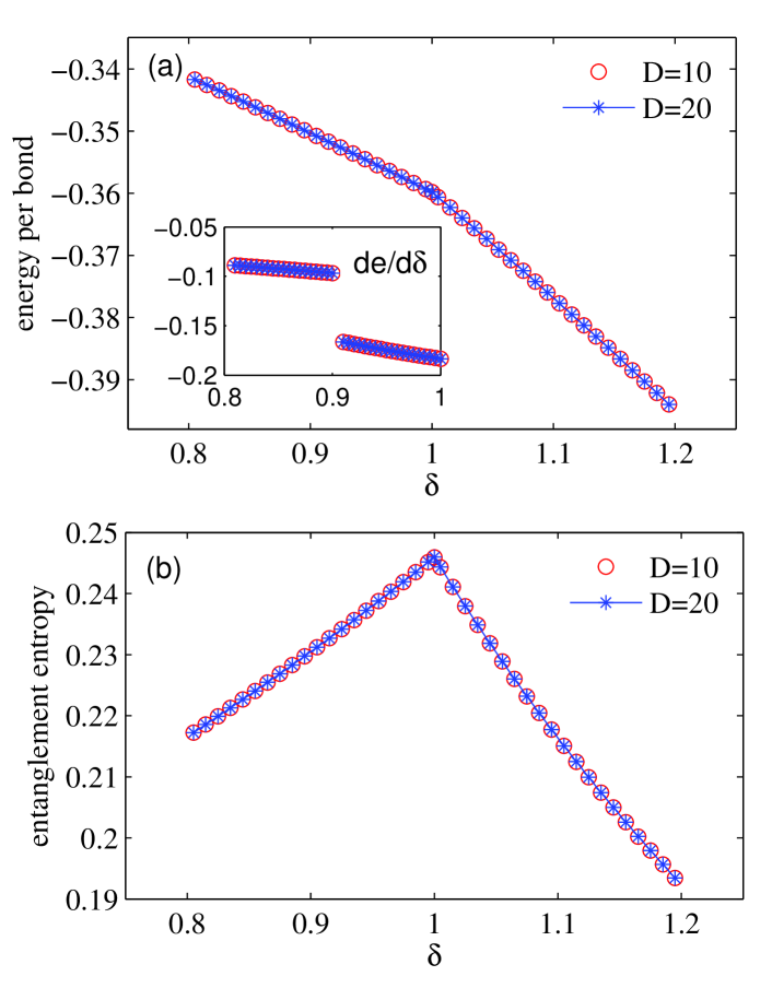
Figure 6 shows the $\delta$-dependence of the ground state energy per bond and the entanglement entropy for the XXZ model. A clear first order quantum phase transition is observed at $\delta=1$. The energy per bond shows a change of slope at $\delta=1$ (the first-order energy derivative is shown in the inset), which suggests that there is an energy level crossing. The entanglement entropy varies continuously across the transition point, but exhibits a cusp.

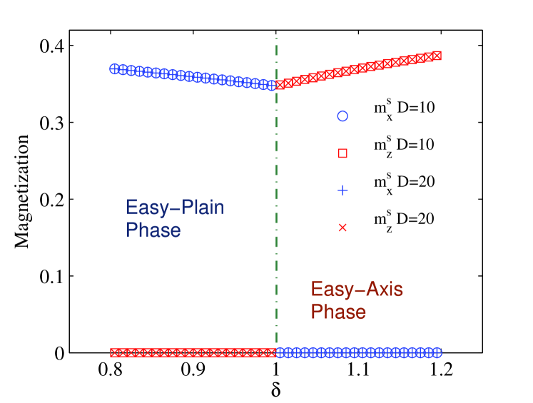
Figure 7 shows the staggered magnetization $m_{x}^{s}$ and $m_{z}^{s}$ around the critical point. The ground state is found to possess in-plane antiferromagnetic order with a finite $m^{s}_{x}$ for $\delta<1$, and $z$-axis antiferromagnetic order with a finite $m^{s}_{z}$ for $\delta>1$. At the transition point, the two order parameters change suddenly, displaying a spin flip transition. This result verifies the conjecture made by Otsuka. Otsuka

At the transition point, we find that the ground state energy per bond has the value $e_{b}=-0.359817(3)$ and the spontaneous magnetization has the value $m_{s}=0.34736(1)$ for $D=40$. The errors in the parentheses are estimated by comparing the results for different bond dimension $D$ and different Trotter slices $\tau$. Our results agree well with the DMRG data published in Ref. [Kumar, ], where the local magnetization is found to be $m=0.347$ on the central lattice site and the bond energy between the central spin and a spin on the first layer is $e=-0.359$. This satisfactory agreement suggests that by calculating the Bethe lattice, we can reproduce the results of local properties in the very center of a large Cayley tree.

Figure 8: (Color online) The one-ring cluster with 12 sites. The diagonal matrices $\Lambda$ are defined on the dangling bonds. The dashed lines represent removed bonds (the physical couplings on the dashed line still exist).

Figure 9: (Color online) The 4-ring cluster with 26 sites. The inequivalent lattice sites are numbered from 1 to 16. $\Lambda_{i,j}$ labels the diagonal matrix on the bond linking sites $i$ and $j$.

Figure 10: (Color online) The ground state energy per site for the Heisenberg model on the honeycomb lattice. The results are evaluated in the central area of the clusters. The dashed line is the recent quantum Monte Carlo result.Low The number of hexagonal rings is used to label the cluster size.

V Cluster update scheme

In the previous sections, the simple update has been applied to study the quantum spin models on the Bethe lattice, leading to very accurate results. What is more, in terms of the Bethe approximation, these results can also be regarded as approximations for the corresponding 2D lattice models. Actually, the simple update scheme has already been used to study regular 2D lattices, such as the honeycomb or square lattices. Combined with the TRG/SRG techniques, it can achieve rather accurate results.Xiang ; Xie ; Zhao Nevertheless, in this section, we would provide a different way of using the simple update to calculate 2D lattices. Inspired by the generalization of the Bethe approximation to larger clusters in classical statistical mechanics,Plischke we apply simple update to various tree tensor clusters. In this way, the advantage (efficiency) in treating a tree tensor network, namely the fact that it can be readily canonicalized, is utilized to improve the calculation accuracy on a regular 2D lattice.

To start, as a first-order approximation, let us compare the results on the $q=3$ Bethe lattice (which has no loops) with those on the 2D honeycomb lattice (whose coordination number is also $q=3$, and it does have loops). Our result for the ground state energy of the Heisenberg model on the $q=3$ Bethe lattice is $e_{b}=-0.359817(3)$, while the corresponding energy on the honeycomb lattice obtained by the recent quantum Monte Carlo calculation is $e_{\rm{QMC}}=-0.36303(14)$. Low The relative difference between these two energies is less than $0.9\%$. However, the spontaneous magnetization for the ground state of the Heisenberg model on the Bethe lattice, namely $m_{s}=0.34736(1)$, is much larger than the corresponding value on the honeycomb lattice, which is about 0.27 as obtained by the quantum Monte Carlo.Low Notice, some other results for the magnetization on the honeycomb or square lattice obtained with the tensor network algorithms are also found to be higher than the Monte Carlo ones.Xiang ; Bauer

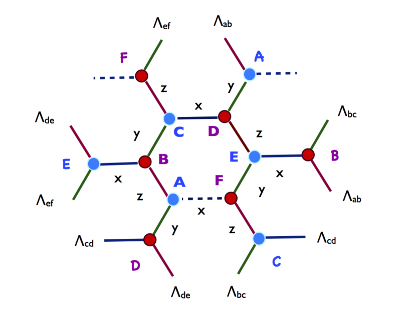
As a next step, our approximate treatment of the 2D honeycomb lattice can be improved by using tensor networks that include rings. In Fig. 8, the cluster with one hexagonal ring is shown, some geometric bonds are removed (dashed lines in Fig. 8) to form a tree tensor cluster. Note although the tensor network does not have geometric bonds on the dashed lines, in the Hamiltonian the couplings along these bonds nevertheless exist. Therefore, the projections by imaginary time evolution should be executed also on the dashed lines. This cannot be done directly as on usual bonds, but can be accomplished as follows with the help of the swap gates. The swap gates are used to exchange the physical indices of two tensors, which proceeds similarly as the projection scheme illustrated in Fig. 2, with the minor revision that the imaginary tim evolving operator $U(\tau)$ is now replaced with a swap operator $U_{s}$, that conducts $U_{s}|m_{i},m_{j}\rangle=|m_{j},m_{i}\rangle$.

In Fig. 8, take the dashed bond between site A and F as an example, swap gates moves the physical index on site A in the order A $\to$ B $\to$ C, and the physical index on site F as F $\to$ E $\to$ D. After that, the two spins are linked by the solid bond between C and D, then we can take the projection and update processes as on an usual bond. After that, we have to move the two spin indices back to their original positions by reversed swap operations, which accomplishes the special projection step on a dashed bond. Through iterative and self-consistent projection processes on the solid and the dashed bonds of the tree cluster, an approximation for 2D lattices can be obtained. Compared with the simple Bethe lattice, this tree tensor cluster approach can provide better approximation for 2D. On the other hand, it can also be regarded as an ideal method for evaluating the “super Bethe lattice”, of which each “single site” is now placed with a hexagonal ring, instead of a single site, and the coordinate number $q=6$.

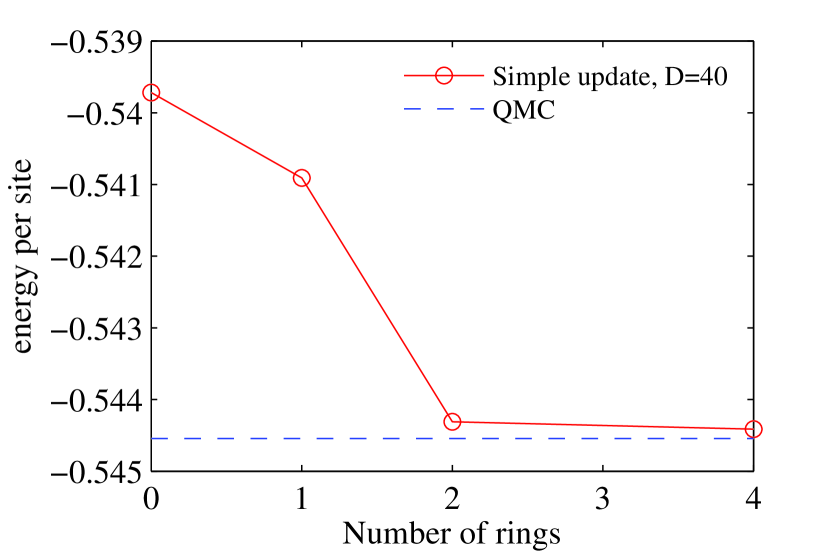
Beyond the one-ring cluster, more rings can be included to further enlarge the cluster. As an example, Fig. 9 shows a cluster with 4 hexagonal rings. The accuracy of energy versus different cluster size (labelled by the number of rings included) are shown in Fig. 10, which verifies that the accuracy could be improved consistently with enhancing the cluster size. To obtain better approximation for true 2D lattices, the local observables are detected in the center area of the cluster. In practice, for the 4-ring tree tensor cluster in Fig. 9, the results are obtained by averaging over sites 3 and 4. We find an energy per site of $e\simeq-0.54441$ (bond energy $e_{b}\simeq-0.36294$) and a local magnetization of $m=[e(h_{s})-e(h_{s}=0)]/h_{s}\simeq 0.3147$ (with a staggered magnetic field $h_{s}=0.01$). Hence, the inclusion of rings clearly improves the agreement with QMC data. For the transverse Ising model, through the 4-ring cluster calculations, the phase transition point is estimated as $h_{c}\simeq 1.1$, which is also more accurate than the simple Bethe approximation. More numerical results with larger clusters and further details of this cluster Bethe approximation will be published separately.

VI Conclusion

In summary, the simple update scheme is employed to study two spin models on the Bethe lattice, i.e., the transverse Ising and the Heisenberg XXZ model. For the Ising model, it is found that the correlation length, as well as the entanglement entropy, does not diverge at the second-order transition point. Through a scale transformation, we have given an intuitive explanation of this peculiar “critical” phenomenon. Moreover, by studying the magnetic susceptibility, we show that the correlation length is upper bounded. For the Heisenberg XXZ model, the existence of a first-order phase transition at the isotropic point is clearly verified, and the two different magnetic ordered phases are identified as the easy-plain and easy-axis phases, respectively. Furthermore, in terms of the Bethe approximation, we obtain accurate and scalable approximations for the 2D lattice models by applying the simple update to tree tensor clusters.

VII Acknowledgement

The authors would like to thank Tomotoshi Nishino and Zhong-Chao Wei for stimulating discussions. WL is also indebted to Gang Su, Cheng Guo, Guang-Hua Liu, Ming-Pu Qin, Li-Ping Yang, and Hui-Hai Zhao for helpful discussions. TX was supported by the National Natural Science Foundation of China (Grants No. 10934008 and No. 10874215) and the MOST 973 Project (Grant No. 2011CB309703). WL was supported by the DFG through SFB-TR12.

References

- (1) Y.-Y. Shi, L.-M. Duan, and G. Vidal, Phys. Rev. A 74, 022320 (2006).
- (2) L. Tagliacozzo, G. Evenbly, and G. Vidal, Phys. Rev. B 80, 235127 (2009).
- (3) V. Murg, F. Verstraete, Ö. Legeza and R.M. Noack, Phys. Rev. B 82, 205105 (2010).
- (4) G. Vidal, Phys. Rev. Lett. 99, 220405 (2007); Phys. Rev. Lett. 101, 110501 (2008).
- (5) F. Verstraete and J. I. Cirac, arXiv:cond-mat/0407066.
- (6) M. Levin and C. P. Nave, Phys. Rev. Lett. 99, 120601 (2007).
- (7) H.C. Jiang, Z.Y. Weng, and T. Xiang, Phys. Rev. Lett. 101, 090603 (2008).
- (8) Z.C. Gu, M. Levin, and X.G. Wen, Phys. Rev. B 78, 205116 (2008); Z.C. Gu and X.G. Wen, Phys. Rev. B 80, 155131 (2009).
- (9) Z.Y. Xie, H.C. Jiang, Q.N. Chen, Z.Y. Weng, and T. Xiang, Phys. Rev. Lett. 103, 160601 (2009).
- (10) H.H. Zhao, Z.Y. Xie, Q.N. Chen, Z.C. Wei, J.W. Cai, and T. Xiang, Phys. Rev. B 81, 174411 (2010).
- (11) S. R. White, Phys. Rev. Lett. 69, 2863 (1992); Phys. Rev. B 48, 10345 (1993).
- (12) P. Chen, C.Y. Lai, and M.F. Yang, J. Stat. Mech. P10001 (2009).
- (13) W. Li, S.-S. Gong, Y. Zhao, and G. Su, Phys. Rev. B 81, 184427 (2010).
- (14) H.H. Zhao, Cenke Xu, Q.N. Chen, Z.C. Wei, M.P. Qin, G.M. Zhang, and T. Xiang, Phys. Rev. B 85, 134416 (2012).
- (15) L. Wang and F. Verstraete, arXiv:1110.4362v.
- (16) H. Bethe, Proc. R. Soc. A 150, 552 (1935).
- (17) M. Plischke and B. Bergersen, Equilibrium Statistical Physics (3rd edition, World Scientific Publishing, Singapore, 2006), Chapter 3, pp. 71-74.
- (18) Rodney J. Baxter, Exactly Solved Models in Statistical Mechanics (Academic Press, 1982), Chapter 4, pp. 47-58.
- (19) M.A. Martin-Delgado, J. Rodriguez-Laguna, and G. Sierra, Phy. Rev. B 65, 155116 (2002).
- (20) D. Astruc, Nat. Chem. 4, 255 (2012).
- (21) H. Otsuka, Phys. Rev. B 53, 14004 (1996).
- (22) B. Friedman, J. Phys.: Condens. Matter 9, 9021 (1997).
- (23) M. Kumar, S. Ramasesha, and Z.G. Soos, Phys. Rev. B 85, 134415 (2012).
- (24) M. Ostilli, Physica A 391, 3417 (2012).
- (25) D. Nagaj, E. Farhi, J. Goldstone, P. Shor, and I. Sylvester, Phys. Rev. B 77, 214431 (2008).
- (26) Á. Nagy, Annals of Physics 327, 54252 (2012).
- (27) G. Vidal, Phys. Rev. Lett. 98, 070201 (2007); R. Orús and G. Vidal, Phys. Rev. B 78, 155117 (2008).
- (28) H.W.J. Blöte and Y. Deng, Phys. Rev. E 66, 066110 (2002).
- (29) We thank Guilhem Semerjian for pointing out to us, after we had made our work public, that this argument had been found previously in the context of Bose Hubbard model on the Beth lattice, in G. Semerjian, M. Tarzia and F. Zamponi, Phys. Rev. B 80, 014524 (2009).
- (30) H.-Q. Lin, J.S. Flynn and D.D. Betts, Phys. Rev. B, 64, 214411 (2001).
- (31) T. Barnes, D. Kotchan, and E.S. Swanson, Phys. Rev. B 39, 4357 (1988).
- (32) R.F. Bishop, D.J.J. Farnell and J.B. Parkinson, J. Phys.: Condens. Matter 8, 11153 (1996).
- (33) R.F. Bishop, D.J.J. Farnell, S.E. Krüger, J.B. Parkinson, J. Richter and C. Zeng, J. Phys.: Condens. Matter 12, 6887 (2000).
- (34) B. Bauer, G. Vidal, M. Troyer, J. Stat. Mech. P09006 (2009).
- (35) Mohamad Al Hajj, Nathalie Guihéry, Jean-Paul Malrieu, and Peter Wind, Phy. Rev. B 70, 094415 (2004).
- (36) H.J. Changlani, S. Ghosh, C.L. Henley, A.M. Laüchli, arXiv:1208.1773v1.
- (37) U. Löw, Condens. Matter Phys. 12, 497 (2009).