A Unified Convergence Analysis of Block Successive Minimization Methods for Nonsmooth Optimization

Abstract

The block coordinate descent (BCD) method is widely used for minimizing a continuous function $f$ of several block variables. At each iteration of this method, a single block of variables is optimized, while the remaining variables are held fixed. To ensure the convergence of the BCD method, the subproblem to be optimized in each iteration needs to be solved exactly to its unique optimal solution. Unfortunately, these requirements are often too restrictive for many practical scenarios. In this paper, we study an alternative inexact BCD approach which updates the variable blocks by successively minimizing a sequence of approximations of $f$ which are either locally tight upper bounds of $f$ or strictly convex local approximations of $f$. We focus on characterizing the convergence properties for a fairly wide class of such methods, especially for the cases where the objective functions are either non-differentiable or nonconvex. Our results unify and extend the existing convergence results for many classical algorithms such as the BCD method, the difference of convex functions (DC) method, the expectation maximization (EM) algorithm, as well as the alternating proximal minimization algorithm.

I Introduction

Consider the following optimization problem

$$\min\quad f(x_{1},\ldots,x_{n})$$

$${\rm s.t.}\quad x_{i}\in\mathcal{X}_{i},\;i=1,2,\ldots,n,$$

where $\mathcal{X}_{i}\subseteq\mathbb{R}^{m_{i}}$ is a closed convex set, and $f:\prod_{i=1}^{n}\mathcal{X}_{i}\to\mathbb{R}$ is a continuous function. A popular approach for solving the above optimization problem is the block coordinate descent method (BCD), which is also known as the Gauss-Seidel method. At each iteration of this method, the function is minimized with respect to a single block of variables while the rest of the blocks are held fixed. More specifically, at iteration $r$ of the algorithm, the block variable $x_{i}$ is updated by solving the following subproblem

$$x_{i}^{r}=\arg\min_{y_{i}\in\mathcal{X}_{i}}\quad f(x_{1}^{r},\ldots,x_{i-1}^{r},y_{i},x_{i+1}^{r-1},\ldots,x_{n}^{r-1}),\quad i=1,2,\ldots,n.$$ (1)

Let us use $\{x^{r}\}$ to denote the sequence of iterates generated by this algorithm, where $x^{r}\triangleq(x_{1}^{r},\ldots,x_{n}^{r})$. Due to its particular simple implementation, the BCD method has been widely used for solving problems such as power allocation in wireless communication systems [28], clustering [14], image denoising and image reconstruction [7] and dynamic programming [17].

Convergence of the BCD method typically requires the uniqueness of the minimizer at each step or the quasi-convexity of the objective function (see [30] and the references therein). Without these assumptions, it is possible that the BCD iterates do not get close to any of the stationary points of the problem (see Powell [24] for examples). Unfortunately, these requirements can be quite restrictive in some important practical problems such the tensor decomposition problem (see [19] and the application section in this work) and the sum rate maximization problem in wireless networks. In fact, for the latter case, even solving the per block subproblem (1) is difficult due to the non-convexity and non-differentiability of the objective function.

To overcome such difficulties, one can modify the BCD algorithm by optimizing a well-chosen approximate version of the objective function at each iteration. The classical gradient descent method, for example, can be viewed as an implementation of such strategy. To illustrate, recall that the update rule of the gradient descent method is given by

$$x^{r+1}=x^{r}-\alpha^{r+1}\nabla f(x^{r}).$$

This update rule is equivalent to solving the following problem

$$x^{r+1}=\arg\min_{x}\quad g(x,x^{r}),$$

where

$$g(x,x^{r})\triangleq f(x^{r})+\nabla f(x^{r})(x-x^{r})+\frac{1}{2\alpha^{r+1}}\|x-x^{r}\|^{2}.$$

Clearly, the function $g(x,x^{r})$ is an approximation of $f(\cdot)$ around the point $x^{r}$. In fact, as we will see later in this paper, successively optimizing an approximate version of the original objective is the key idea of many important algorithms such as the concave-convex procedure [33], the EM algorithm [10], the proximal minimization algorithm [2], to name a few. Furthermore, this idea can be used to simplify the computation and to guarantee the convergence of the original BCD algorithm with the Gauss-Seidel update rule (e.g. [31], [12],[32]). However, despite its wide applicability, there appears to be no general unifying convergence analysis for this class of algorithms.

In this paper, we provide a unified convergence analysis for a general class of inexact BCD methods in which a sequence of approximate versions of the original problem are solved successively. Our focus will be on problems with nonsmooth and nonconvex objective functions. Two types of approximations are considered: one being a locally tight upper bound for the original objective function, the other being a convex local approximation of the objective function. We provide convergence analysis for both of these successive approximation strategies as well as for various types of updating rules, including the cyclic updating rule, the Gauss-Southwell update rule or the overlapping essentially cyclic update rule. By allowing inexact solution of subproblems, our work unifies and extends several existing algorithms and their convergence analysis, including the difference of convex functions (DC) method, the expectation maximization (EM) algorithm, as well as the alternating proximal minimization algorithm.

II Technical Preliminaries

Throughout the paper, we adopt the following notations. We use $\mathbb{R}^{m}$ to denote the space of $m$ dimensional real valued vectors, which is also represented as the Cartesian product of $n$ smaller real valued vector spaces, i.e.,

$$\mathbb{R}^{m}=\mathbb{R}^{m_{1}}\times\mathbb{R}^{m_{2}}\times\ldots\times\mathbb{R}^{m_{n}},$$

where $\sum_{i=1}^{n}m_{i}=m$. We use the notation $(0,\ldots,d_{k},\ldots,0)$ to denote the vector of all zeros except the $k$-th block, with $d_{k}\in\mathbb{R}^{m_{k}}$. The following concepts/definitions are adopted in our paper:

• Distance of a point from a set: Let $\mathcal{S}\subseteq\mathbb{R}^{m}$ be a set and $x$ be a point in $\mathbb{R}^{m}$, the distance of the point $x$ from the set $\mathcal{S}$ is defined as

  $$d(x,\mathcal{S})=\inf_{s\in\mathcal{S}}\|x-s\|,$$

  where $\|\cdot\|$ denotes the 2-norm in $\mathbb{R}^{m}$.

• Directional derivative: Let $f:\mathcal{D}\rightarrow\mathbb{R}$ be a function where $\mathcal{D}\subseteq\mathbb{R}^{m}$ is a convex set. The directional derivative of $f$ at point $x$ in direction $d$ is defined by

  $$f^{\prime}(x;d)\triangleq\liminf_{\lambda\downarrow 0}\frac{f(x+\lambda d)-f(x)}{\lambda}.$$

• Stationary points of a function: Let $f:\mathcal{D}\rightarrow\mathbb{R}$ be a function where $\mathcal{D}\subseteq\mathbb{R}^{m}$ is a convex set. The point $x$ is a stationary point of $f(\cdot)$ if $f^{\prime}(x;d)\geq 0$ for all $d$ such that $x+d\in\mathcal{D}$. In this paper we use the notation $\mathcal{X}^{*}$ to denote the set of stationary points of a function.

• Regularity of a function at a point: The function $f:\mathbb{R}^{m}\rightarrow\mathbb{R}$ is regular at the point $z\in{\rm dom}f$ with respect to the coordinates $m_{1},m_{2},\ldots,m_{n}$, $m_{1}+m_{2}+\ldots+m_{n}=m$, if $f^{\prime}(z;d)\geq 0$ for all $d=(d_{1},d_{2},\ldots,d_{n})$ with $f^{\prime}(z;d_{k}^{0})\geq 0$, where $d_{k}^{0}=(0\ldots,d_{k},\ldots,0)$ and $d_{k}\in\mathbb{R}^{m_{k}},\forall\;k$. For detailed discussion on the regularity of a function, the readers are referred to [30, Lemma 3.1].

• Quasi-convex function: The function $f$ is quasi-convex if

  $$f(\theta x+(1-\theta)y)\leq\max\{f(x),f(y)\},\quad\forall\;\theta\in(0,1),\ \forall\;x,y\in\;{\rm dom}\;f$$

• Coordinatewise minimum of a function: $z\in{\rm dom}\;f\subseteq\mathbb{R}^{m}$ is coordinatewise minimum of $f$ with respect to the coordinates in $\Re^{m_{1}},\Re^{m_{2}},\ldots,\Re^{m_{n}}$, $m_{1}+\ldots+m_{k}=m$ if

  $$f(z+(0,\ldots,d_{k},\ldots,0))\geq f(z),\quad\forall\;d_{k}\in\mathbb{R}^{m_{k}}\quad{\rm with}\quad z+(0,\ldots,d_{k},\ldots,0)\in\;{\rm dom}\;f.$$

III Successive Upper-bound Minimization (SUM)

To gain some insights to the general inexact BCD method, let us first consider a simple Successive Upper-bound Minimization (SUM) approach in which all the variables are grouped into a single block. Although simple in form, the SUM algorithm is the key to many important algorithms such as the DC programming [33] and the EM algorithm [4].

Consider the following optimization problem

$$\begin{split}\min\quad&f(x)\\ {\rm s.t.}\quad&x\in\mathcal{X},\end{split}$$ (2)

where $\mathcal{X}$ is a closed convex set. Without loss of generality, we can assume that ${\rm dom}\;f=\mathcal{X}$. When the objective function $f(\cdot)$ is non-convex and/or nonsmooth, solving (2) directly may not be easy. The SUM algorithm circumvents such difficulty by optimizing a sequence of approximate objective functions instead. More specifically, starting from a feasible point $x^{0}$, the algorithm generates a sequence $\{x^{r}\}$ according to the following update rule

$$x^{r}\in\arg\min_{x\in\mathcal{X}}\quad u(x,x^{r-1})$$ (3)

where $x^{r-1}$ is the point generated by the algorithm at iteration $r-1$ and $u(x,x^{r-1})$ is an approximation of $f(x)$ at the $r$-th iteration. Typically the approximate function $u(\cdot,\cdot)$ needs to be chosen such that the subproblem (3) is easy to solve. Moreover, to ensure the convergence of the SUM algorithm, certain regularity conditions on $u(\cdot,\cdot)$ is required (which will be discussed shortly). Among others, $u(x,x^{r-1})$ needs to be a global upper bound for $f(x)$, hence the name of the algorithm. The main steps of the SUM algorithm are presented in Fig. 1.

1 Find a feasible point $x^{0}\in\mathcal{X}$ and set $r=0$ 2 repeat 3 $r=r+1$ 4 Let $\mathcal{X}^{r}=\arg\min_{x\in\mathcal{X}}u(x,x^{r-1})$ 5 Set $x^{r}$ to be an arbitrary element in $\mathcal{X}^{r}$ 6 until some convergence criterion is met

Figure 1: Pseudo code of the SUM algorithm

We remark that the proposed SUM algorithm is in many ways similar to the inner approximation algorithm (IAA) developed in [21], with the following key differences:

• The IAA algorithm approximates both the objective functions and the feasible sets. On the contrary, the SUM algorithm only approximates the objective function.

• The the IAA algorithm is only applicable for problems with smooth objectives, while the SUM algorithm is able to handle nonsmooth objectives as well.

It is worth mentioning that the existing convergence result for the IAA algorithm is quite weak. In particular, [21, Theorem 1] states that if the whole sequence converges, then the algorithm should converge to a stationary point. In the following, we show that the SUM algorithm provides stronger convergence guarantees as long as the approximation function $u(\cdot,\cdot)$ satisfies certain mild assumptions which we outline below.

Assumption 1

Let the approximation function $u(\cdot,\cdot)$ satisfy the following

$$u(y,y)=f(y),\quad\forall\;y\in\mathcal{X}$$ (A1)

$$u(x,y)\geq f(x),\quad\forall\;x,y\in\mathcal{X}$$ (A2)

$$u^{\prime}(x,y;d)\bigg{|}_{x=y}=f^{\prime}(y;d),\quad\forall\;d\;\;{\rm with}\;\;y+d\in\mathcal{X}$$ (A3)

$$u(x,y)\;{\rm is}\;{\rm continuous}\;{\rm in}\;(x,y)$$ (A4)

The assumptions (A1) and (A2) imply that the approximate function $u(\cdot,x^{r-1})$ in (3) is a tight upper bound of the original function. The assumption (A3) guarantees that the first order behavior of $u(\cdot,x^{r-1})$ is the same as $f(\cdot)$ locally (note that the directional derivative $u^{\prime}(x,y;d)$ is only with respect to the variable $x$). Although directly checking (A3) may not be easy, the following proposition provides a sufficient condition under which (A3) holds true automatically.

Proposition 1

Assume $f(x)=f_{0}(x)+f_{1}(x)$, where $f_{0}(\cdot)$ is continuously differentiable and the directional derivative of $f_{1}(\cdot)$ exists at every point $x\in\mathcal{X}$. Consider $u(x,y)=u_{0}(x,y)+f_{1}(x)$, where $u_{0}(x,y)$ is a continuously differentiable function satisfying the following conditions

$$u_{0}(y,y)=f_{0}(y),\quad\forall\;y\in\mathcal{X}$$ (4)

$$u_{0}(x,y)\geq f_{0}(x),\quad\forall\;x,y\in\mathcal{X}.$$ (5)

Then, (A1), (A2) and (A3) hold for $u(\cdot,\cdot)$.

Proof.

First of all, (4) and (5) imply (A1) and (A2) immediately. Now we prove (A3) by contradiction. Assume the contrary so that there exist a $y\in\mathcal{X}$ and a $d\in\mathbb{R}^{m}$ so that

$$f^{\prime}(y;d)\neq u^{\prime}(x,y;d)\bigg{|}_{x=y}\quad{\rm and}\quad y+d\in\mathcal{X}.$$ (6)

This further implies that

$$f_{0}^{\prime}(y;d)\neq u_{0}^{\prime}(x,y;d)\bigg{|}_{x=y}.$$

Furthermore, since $f_{0}(\cdot)$ and $u_{0}(\cdot,\cdot)$ are continuously differentiable, there exists a $\alpha>0$ such that for $z=y+\alpha d$,

$$f^{\prime}_{0}(z;d)\neq u^{\prime}_{0}(x,z;d)\bigg{|}_{x=z}.$$ (7)

The assumptions (4) and (5) imply that

$$\begin{split}u^{\prime}_{0}(x,z;d)\bigg{|}_{x=z}&=\lim_{\lambda\downarrow 0}\frac{u_{0}(z+\lambda d,z)-u_{0}(z,z)}{\lambda}\\ &\geq\lim_{\lambda\downarrow 0}\frac{f_{0}(z+\lambda d)-f_{0}(z)}{\lambda}=f^{\prime}(z;d).\end{split}$$ (8)

On the other hand, the differentiability of $f_{0}(\cdot)$, $u_{0}(\cdot,\cdot)$ and using (4), (5) imply

$$\begin{split}u^{\prime}_{0}(x,z;d)\bigg{|}_{x=z}&=\lim_{\lambda\downarrow 0}\frac{u_{0}(z,z)-u_{0}(z-\lambda d,z)}{\lambda}\\ &\leq\lim_{\lambda\downarrow 0}\frac{f_{0}(z)-f_{0}(z-\lambda d)}{\lambda}=f^{\prime}(z;d).\end{split}$$ (9)

Clearly, (8) and (9) imply that $u^{\prime}_{0}(x,z;d)\bigg{|}_{x=z}=f^{\prime}(z;d)$ which contradicts (7). ∎

The following theorem establishes the convergence for the SUM algorithm.

Theorem 1

Assume that Assumption 1 is satisfied. Then every limit point of the iterates generated by the SUM algorithm is a stationary point of the problem (2).

Proof.

Firstly, we observe the following series of inequalities

$$f(x^{r+1})\stackrel{{\scriptstyle\rm(i)}}{{\leq}}u(x^{r+1},x^{r})\stackrel{{\scriptstyle\rm(ii)}}{{\leq}}u(x^{r},x^{r})=f(x^{r}),\quad\forall\;r=0,1,2,\ldots$$ (10)

where step ${\rm(i)}$ is due to (A1), step ${\rm(ii)}$ follows from the optimality of $x^{t+1}$ (cf. step 4 and 5 in Fig.1), and the last equality is due to (A2). A straightforward consequence of (10) is that the sequence of the objective function values are non-increasing, that is

$$f(x^{0})\geq f(x^{1})\geq f(x^{2})\geq\ldots$$ (11)

Assume that there exists a subsequence $\{x^{r_{j}}\}$ converging to a limit point $z$. Then Assumptions (A1), (A2) together with (11) imply that

$$u(x^{r_{j+1}},x^{r_{j+1}})=f(x^{r_{j+1}})\leq f(x^{r_{j}+1})\leq u(x^{r_{j}+1},x^{r_{j}})\leq u(x,x^{r_{j}}),\quad\forall\;x\in\mathcal{X}$$

Letting $j\rightarrow\infty$, we obtain

$$u(z,z)\leq u(x,z),\quad\forall\;x\in\mathcal{X},$$

which implies

$$u^{\prime}(x,z;d)\bigg{|}_{x=z}\geq 0,\quad\forall\;d\in\mathbb{R}^{m}\;\;{\rm with}\;\;z+d\in\mathcal{X}.$$

Combining with (A3), we obtain

$$f^{\prime}(z;d)\geq 0,\quad\forall\;d\in\mathbb{R}^{m}\;\;{\rm with}\;\;z+d\in\mathcal{X},$$

implying that $z$ is a stationary point of $f(\cdot)$. ∎

Corollary 1

Assume that the level set $\mathcal{X}^{0}=\{x\mid f(x)\leq f(x^{0})\}$ is compact and Assumption 1 holds. Then, the sequence of iterates $\{x^{r}\}$ generated by the SUM algorithm satisfy

$$\lim_{r\rightarrow\infty}\quad d(x^{r},\mathcal{X}^{*})=0,$$

where $\mathcal{X}^{*}$ is the set of stationary points of (2).

Proof.

We prove the claim by contradiction. Suppose on the contrary that there exists a subsequence $\{x^{r_{j}}\}$ such that $d(x^{r_{j}},\mathcal{X}^{*})\geq\gamma$ for some $\gamma>0$. Since the sequence $\{x^{r_{j}}\}$ lies in the compact set $X^{0}$, it has a limit point $z$. By further restricting the indices of the subsequence, we obtain

$$d(z,\mathcal{X}^{*})=\lim_{j\rightarrow\infty}d(x^{r_{j}},\mathcal{X}^{*})\geq\gamma,$$

which contradicts the fact that $z\in\mathcal{X}^{*}$ due to Theorem 1. ∎

The above results show that under Assumption 1, the SUM algorithm is globally convergent. In the rest of this work, we derive similar results for a family of more general inexact BCD algorithms.

IV The Block Successive Upper-bound Minimization Algorithm

In many practical applications, the optimization variables can be decomposed into independent blocks. Such block structure, when judiciously exploited, can lead to low-complexity algorithms that are distributedly implementable. In this section, we introduce the Block Successive Upper-bound Minimization (BSUM) algorithm, which effectively takes such block structure into consideration.

Let us assume that the feasible set $\mathcal{X}$ is the cartesian product of $n$ closed convex sets: $\mathcal{X}=\mathcal{X}_{1}\times\ldots\times\mathcal{X}_{n}$, with $\mathcal{X}_{i}\subseteq\mathbb{R}^{m_{i}}$ and $\sum_{i}m_{i}=m$. Accordingly, the optimization variable $x\in\mathbb{R}^{m}$ can be decomposed as: $x=(x_{1},x_{2},\ldots,x_{n})$, with $x_{i}\in\mathcal{X}_{i},~{}i=1,\cdots,M$. We are interested in solving the problem

$$\begin{split}\min\quad&f(x)\\ {\rm s.t.}\quad&x\in\mathcal{X}.\end{split}$$ (12)

Different from the SUM algorithm, the BSUM algorithm only updates a single block of variables in each iteration. More precisely, at iteration $r$, the selected block (say block $i$) is computed by solving the following subproblem

$$\begin{split}\min_{x_{i}}\quad&u_{i}(x_{i},x^{r-1})\\ {\rm s.t.}\quad&x_{i}\in\mathcal{X}_{i},\end{split}$$ (13)

where $u_{i}(\cdot,x^{r-1})$ is again an approximation (in fact, a global upper-bound) of the original objective $f(\cdot)$ at the point $x^{r-1}$. Fig. 2 summarizes the main steps of the BSUM algorithm. Note that although the blocks are updated following a simple cyclic rule, the algorithm and its convergence results can be easily extended to the (more general) essentially cyclic update rule as well. This point will be further elaborated in Section VII.

1 Find a feasible point $x^{0}\in\mathcal{X}$ and set $r=0$ 2 repeat 3 $r=r+1$, $i=(r\;{\rm mod}\;n)+1$ 4 Let $\mathcal{X}^{r}=\arg\min_{x_{i}\in\mathcal{X}_{i}}u_{i}(x_{i},x^{r-1})$ 5 Set $x_{i}^{r}$ to be an arbitrary element in $\mathcal{X}^{r}$ 6 Set $x_{k}^{r}=x_{k}^{r-1},\quad\forall\;k\neq i$ 7 until some convergence criterion is met

Figure 2: Pseudo code of the BSUM algorithm

Now we are ready to study the convergence behavior of the BSUM algorithm. To this end, the following regularity conditions on the function $u_{i}(\cdot,\cdot)$ are needed.

Assumption 2

$$u_{i}(y_{i},y)=f(y),\quad\forall\;y\in\mathcal{X},\forall\;i$$ (B1)

$$u_{i}(x_{i},y)\geq f(y_{1},\ldots,y_{i-1},x_{i},y_{i+1},\ldots,y_{n}),\quad\;\forall\;x_{i}\in\mathcal{X}_{i},\forall\;y\in\mathcal{X},\forall\;i$$ (B2)

$$u_{i}^{\prime}(x_{i},y;d_{i})\bigg{|}_{x_{i}=y_{i}}=f^{\prime}(y;d),\quad\forall\;d=(0,\ldots,d_{i},\ldots,0)\;\;{\rm s.t.}\;\;y_{i}+d_{i}\in\mathcal{X}_{i},\forall\;i$$ (B3)

$$u_{i}(x_{i},y)\;{\rm is}\;{\rm continuous}\;{\rm in}\;(x_{i},y),\quad\forall\;i$$ (B4)

Similar to Proposition 1, we can identify a sufficient condition to ensure (B3).

Proposition 2

Assume $f(x)=f_{0}(x)+f_{1}(x)$, where $f_{0}(\cdot)$ is continuously differentiable and the directional derivative of $f_{1}(\cdot)$ exists at every point $x\in\mathcal{X}$. Consider $u_{i}(x_{i},y)=u_{0,i}(x_{i},y)+f_{1}(x)$, where $u_{0,i}(x_{i},y)$ satisfies the following assumptions

$$u_{0,i}(x_{i},x)=f_{0}(x),\quad\forall\;x\in\mathcal{X},\quad\forall\;i$$

$$u_{0,i}(x_{i},y)\geq f_{0}(y_{1},\ldots,y_{i-1},x_{i},y_{i+1},\ldots,y_{n}),\;\forall\;x,y\in\mathcal{X}\quad\forall\;i.$$

Then, (B1), (B2), and (B3) hold.

Proof.

The proof is exactly the same as the proof in Proposition 1. ∎

The convergence results regarding to the BSUM algorithm consist of two parts. In the first part, a quasi-convexity of the objective function is assumed, which guarantees the existence of the limit points. This is in the same spirit of the classical proof of convergence for the BCD method in [2]. However, if we know that the iterates lie in a compact set, then a stronger result can be proved. Indeed, in the second part of the theorem, the convergence is obtained by relaxing the quasi-convexity assumption while imposing the compactness assumption of level sets.

Theorem 2

• Suppose that the function $u_{i}(x_{i},y)$ is quasi-convex in $x_{i}$ and Assumption 2 holds. Furthermore, assume that the subproblem (13) has a unique solution for any point $x^{r-1}\in\mathcal{X}$. Then, every limit point $z$ of the iterates generated by the BSUM algorithm is a coordinatewise minimum of (12). In addition, if $f(\cdot)$ is regular at $z$, then $z$ is a stationary point of (12).

• Suppose the level set $\mathcal{X}^{0}=\{x\mid f(x)\leq f(x^{0})\}$ is compact and Assumption 2 holds. Furthermore, assume that the subproblem (13) has a unique solution for any point $x^{r-1}\in\mathcal{X}$ for at least $n-1$ blocks. If $f(\cdot)$ is regular at every point in the set of stationary points $\mathcal{X}^{*}$ with respect to the coordinates $x_{1},\ldots,x_{n}$. Then, the iterates generated by the BSUM algorithm converge to the set of stationary points, i.e.,

  $$\lim_{r\rightarrow\infty}\quad d(x^{r},\mathcal{X}^{*})=0.$$

Proof.

The proof of part (a) is similar to the one in [2] for block coordinate descent approach. First of all, since a locally tight upper bound of $f(\cdot)$ is minimized at each iteration, we have

$$f(x^{0})\geq f(x^{1})\geq f(x^{2})\geq\ldots.$$ (14)

Therefore, the continuity of $f(\cdot)$ implies

$$\lim_{r\rightarrow\infty}f(x^{r})=f(z).$$ (15)

Let us consider the subsequence $\{x^{r_{j}}\}$ converging to the limit point $z$. Since the number of blocks is finite, there exists a block which is updated infinitely often in the subsequence $\{r_{j}\}$. Without loss of generality, we assume that block $n$ is updated infinitely often. Thus, by further restricting to a subsequence, we can write

$$x_{n}^{r_{j}}=\arg\min_{x_{n}}\quad u_{n}(x_{n},x^{r_{j}-1}).$$

Now we prove that $x^{r_{j}+1}\rightarrow z$, in other words, we will show that $x_{1}^{r_{j}+1}\rightarrow z_{1}$. Assume the contrary that $x_{1}^{r_{j}+1}$ does not converge to $z_{1}$. Therefore by further restricting to a subsequence, there exists $\bar{\gamma}>0$ such that

$$\bar{\gamma}\leq\gamma^{r_{j}}=\|x_{1}^{r_{j}+1}-x_{1}^{r_{j}}\|,\ \forall~{}r_{j}.$$

Let us normalize the difference between $x_{1}^{r_{j}}$ and $x_{1}^{r_{j}+1}$, i.e.,

$$s^{r_{j}}\triangleq\frac{x_{1}^{r_{j}+1}-x_{1}^{r_{j}}}{\gamma^{r_{j}}}.$$

Notice that $\|s^{r_{j}}\|=1$, thus $s^{r_{j}}$ belongs to a compact set and it has a limit point $\bar{s}$. By further restricting to a subsequence that converges to $\bar{s}$, using (B1) and (B2), we obtain

$$f(x^{r_{j}+1}) \leq u_{1}(x_{1}^{r_{j}+1},x^{r_{j}})$$ (16)

$$=u_{1}(x_{1}^{r_{j}}+\gamma^{r_{j}}s^{r_{j}},x^{r_{j}})$$ (17)

$$\leq u_{1}(x_{1}^{r_{j}}+\epsilon\bar{\gamma}s^{r_{j}},x^{r_{j}}),\quad\forall\;\epsilon\in[0,1]$$ (18)

$$\leq u_{1}(x^{r_{j}}_{1},x^{r_{j}})$$ (19)

$$=f(x^{r_{j}}),$$ (20)

where (16) and (20) hold due to (B1) and (B2). The inequalities (18) and (19) are the result of quasi-convexity of $u(\cdot,x^{r_{j}})$. Letting $j\rightarrow\infty$ and combining (16), (18), (15), and (20) imply

$$f(z)\leq u_{1}(z_{1}+\epsilon\bar{\gamma}\bar{s},z)\leq f(z),\quad\forall\;\epsilon\in[0,1],$$

or equivalently

$$f(z)=u_{1}(z_{1}+\epsilon\bar{\gamma}\bar{s},z),\quad\forall\;\epsilon\in[0,1].$$ (21)

Furthermore,

$$u_{1}(x_{1}^{r_{j+1}},x^{r_{j+1}}) =f(x^{r_{j+1}})\leq f(x^{r_{j}+1})$$

$$\leq u_{1}(x_{1}^{r_{j}+1},x^{r_{j}})\leq u_{1}(x_{1},x^{r_{j}}),\quad\forall\;x_{1}\in\mathcal{X}_{1}.$$

Letting $j\rightarrow\infty$, we obtain

$$u_{1}(z_{1},z)\leq u_{1}(x_{1},z),\quad\forall\;x_{1}\in\mathcal{X}_{1},$$

which further implies that $z_{1}$ is the minimizer of $u_{1}(\cdot,z)$. On the other hand, we assume that the minimizer is unique, which contradicts (21). Therefore, the contrary assumption is not true, i.e., $x^{r_{j}+1}\rightarrow z$.

Since $x_{1}^{r_{j}+1}=\arg\min_{x_{1}\in\mathcal{X}_{1}}\quad u_{1}(x_{1},x^{r_{j}})$, we get

$$u_{1}(x_{1}^{r_{j}+1},x^{r_{j}})\leq u_{1}(x_{1},x^{r_{j}})\quad\forall\;x_{1}\in\mathcal{X}_{1}.$$

Taking the limit $j\rightarrow\infty$ implies

$$u_{1}(z_{1},z)\leq u_{1}(x_{1},z)\quad\forall\;x_{1}\in\mathcal{X}_{1},$$

which further implies

$$u_{1}^{\prime}(x_{1},z;d_{1})\bigg{|}_{x_{1}=z_{1}}\geq 0,\quad\forall\;d_{1}\in\mathbb{R}^{m_{1}}\quad{\rm with}\quad z_{1}+d_{1}\in\mathcal{X}_{1}.$$

Similarly, by repeating the above argument for the other blocks, we obtain

$$u^{\prime}_{k}(x_{k},z;d_{k})\bigg{|}_{x_{k}=z_{k}}\geq 0,\quad\forall\;d_{k}\in\mathbb{R}^{m_{k}}\quad{\rm with}\quad d_{k}+z_{k}\in\mathcal{X}_{k},\quad\quad\forall\;k=1,\ldots,n.$$ (22)

Combining (B3) and (22) implies

$$f^{\prime}(z;d)\geq 0,\quad\forall\;d=(0,\ldots,d_{k},\ldots,0)\quad{\rm s.t.}\quad d+z\in\mathcal{X},\;\forall\;k$$

in other words, $z$ is the coordinatewise minimum of $f(\cdot)$.

Now we prove part (b) of the theorem. Without loss of generality, let us assume that (13) has a unique solution at every point $x^{r-1}$ for $i=1,2,\ldots,n-1$. Since the iterates lie in a compact set, we only need to show that every limit point of the iterates is a stationary point of $f(\cdot)$. To do so, let us consider a subsequence $\{x^{r_{j}}\}$ which converges to a limit point $z\in\mathcal{X}^{0}\subseteq\mathcal{X}$. Since the number of blocks is finite, there exists a block $i$ which is updated infinitely often in the subsequence $\{x^{r_{j}}\}$. By further restricting to a subsequence, we can assume that

$$x_{i}^{r_{j}}\in\arg\min_{x_{i}}\quad u_{i}(x_{i},x^{r_{j}-1}).$$

Since all the iterates lie in a compact set, we can further restrict to a subsequence such that

$$\lim_{j\rightarrow\infty}\quad x^{r_{j}-i+k}=z^{k},\quad\forall\;k=0,1,\ldots,n,$$

where $z^{k}\in\mathcal{X}^{0}\subseteq\mathcal{X}$ and $z^{i}=z$. Moreover, due to the update rule in the algorithm, we have

$$u_{k}(x_{k}^{r_{j}-i+k},x^{r_{j}-i+k-1})\leq u_{k}(x_{k},x^{r_{j}-i+k-1}),\quad\forall\;x_{k}\in\mathcal{X}_{k},\quad\quad k=1,2,\ldots,n.$$

Taking the limit $j\rightarrow\infty$, we obtain

$$u_{k}(z_{k}^{k},z^{k-1})\leq u_{k}(x_{k},z^{k-1}),\quad\forall\;x_{k}\in\mathcal{X}_{k},\quad\quad k=1,2,\ldots,n.$$ (23)

Combining (23), (B1) and (B2) implies

$$f(z^{k})\leq u_{k}(z_{k}^{k},z^{k-1})\leq u_{k}(z_{k}^{k-1},z^{k-1})=f(z^{k-1}),\quad k=1,\ldots,n.$$ (24)

On the other hand, the objective function is non-increasing in the algorithm and it has a limit. Thus,

$$f(z^{0})=f(z^{1})=\ldots=f(z^{n}).$$ (25)

Using (24), (25), and (23), we obtain

$$f(z)=u_{k}(z_{k}^{k},z^{k-1})\leq u_{k}(x_{k},z^{k-1}),\;\forall\;x_{k}\in\mathcal{X}_{k},\quad k=1,2,\ldots,n.$$ (26)

Furthermore, $f(z)=f(z^{k-1})=u_{k}(z_{k}^{k-1},z^{k-1})$ and therefore,

$$u_{k}(z_{k}^{k-1},z^{k-1})\leq u_{k}(x_{k},z^{k-1}),\;\forall\;x_{k}\in\mathcal{X}_{k},\quad k=1,2,\ldots,n.$$ (27)

The inequalities $\eqref{eq:temp1Thm2}$ and (27) imply that $z_{k}^{k-1}$ and $z_{k}^{k}$ are both the minimizer of $u_{k}(\cdot,z^{k-1})$. However, according to our assumption, the minimizer is unique for $k=1,2,\ldots,n-1$ and therefore,

$$z^{0}=z^{1}=z^{2}=\ldots=z^{n-1}=z$$

Plugging the above relation in (23) implies

$$u_{k}(z_{k},z)\leq u_{k}(x_{k},z),\;\forall\;x_{k}\in\mathcal{X}_{k},\quad k=1,2,\ldots,n-1.$$ (28)

Moreover, by setting $k=n$ in (27), we obtain

$$u_{n}(z_{n},z)\leq u_{n}(x_{n},z),\quad\forall\;x_{n}\in\mathcal{X}_{n}.$$ (29)

The inequalities (28) and (29) imply that

$$u^{\prime}_{k}(x_{k},z;d_{k})\bigg{|}_{x_{k}=z_{k}}\geq 0,\quad\forall\;d_{k}\in\mathbb{R}^{m_{k}}\;{\rm with}\;z_{k}+d_{k}\in\mathcal{X}_{k},\quad k=1,2,\ldots,n.$$

Combining this with (B3) yields

$$f^{\prime}(z;d)\geq 0,\quad\forall\;d=(0,\ldots,d_{k},\ldots,0)\;\;{\rm with}\;\;z_{k}+d_{k}\in\mathcal{X}_{k},\quad k=1,2,\ldots,n,$$

which implies the stationarity of the point $z$ due to the regularity of $f(\cdot)$. ∎

The above result extends the existing result of block coordinate descent method [2] and [30] to the BSUM case where only an approximation of the objective function is minimized at each iteration. As we will see in Section VIII, our result implies the global convergence of several existing algorithms including the EM algorithm or the DC method when the Gauss-Seidel update rule is used.

V The Maximum Improvement Successive Upper-bound Minimization Algorithm

A key assumption for the BSUM algorithm is the uniqueness of the minimizer of the subproblem. This assumption is necessary even for the simple BCD method [2]. In general, by removing such assumption, the convergence is not guaranteed (see [24] for examples) unless we assume pseudo convexity in pairs of the variables [34], [30]. In this section, we explore the possibility of removing such uniqueness assumption.

Recently, Chen et al. [1] have proposed a related Maximum Block Improvement (MBI) algorithm, which differs from the conventional BCD algorithm only by its update schedule. More specifically, only the block that provides the maximum improvement is updated at each step. Remarkably, by utilizing such modified updating rule (which is similar to the well known Gauss-Southwell update rule), the per-block subproblems are allowed to have multiple solutions. Inspired by this recent development, we propose to modify the BSUM algorithm similarly by simply updating the block that gives the maximum improvement. We name the resulting algorithm the Maximum Improvement Successive Upper-bound Minimization (MISUM) algorithm, and list its main steps in Fig. 3.

1 Find a feasible point $x^{0}\in\mathcal{X}$ and set $r=0$ 2 repeat 3 $r=r+1$ 4 Let $k=\arg\min_{i}\min_{x_{i}}u_{i}(x_{i},x^{r-1})$ 5 Let $\mathcal{X}^{r}=\arg\min_{x_{k}\in\mathcal{X}_{k}}u_{k}(x_{k},x^{r-1})$ 6 Set $x_{k}^{r}$ to be an arbitrary element in $\mathcal{X}^{r}$ 7 Set $x_{i}^{r}=x_{i}^{r-1},\quad\forall\;i\neq k$ 8 until some convergence criterion is met

Figure 3: Pseudo code of the MISUM algorithm

Clearly the MISUM algorithm is more general than the MBI method proposed in [1], since only an approximate version of the subproblem is solved at each iteration. Theorem 3 states the convergence result for the proposed MISUM algorithm.

Theorem 3

Suppose that Assumption 2 is satisfied. Then, every limit point $z$ of the iterates generated by the MISUM algorithm is a coordinatewise minimum of (12). In addition, if $f(\cdot)$ is regular at $z$, then $z$ is a stationary point of (12).

Proof.

Let us define $R_{i}(y)$ to be the minimum objective value of the $i$-th subproblem at a point $y$, i.e.,

$$R_{i}(y)\triangleq\min_{x_{i}}\quad u_{i}(x_{i},y).$$

Using a similar argument as in Theorem 2, we can show that the sequence of the objective function values are non-increasing, that is

$$f(x^{r})=u_{i}(x_{i}^{r},x^{r})\geq R_{i}(x^{r})\geq f(x^{r+1}).$$

Let $\{x^{r_{j}}\}$ be the subsequence converging to a limit point $z$. For every fixed block index $i=1,2,\ldots,n$ and every $x_{i}\in\mathcal{X}_{i}$, we have the following series of inequalities

$$u_{i}(x_{i},x^{r_{j}}) \geq R_{i}(x^{r_{j}})$$

$$\geq u_{k}(x_{k}^{r_{j}+1},x^{r_{j}})$$

$$\geq f(x^{r_{j}+1})$$

$$\geq f(x^{r_{j+1}})$$

$$=u_{i}(x_{i}^{r_{j+1}},x^{r_{j+1}}),$$

where we use $k$ to index the block that provides the maximum improvement at iteration $r_{j}+1$. The first and the second inequalities are due to the definition of the function $R_{i}(\cdot)$ and the MISUM update rule, respectively. The third inequality is implied by the upper bound assumption (B2), while the last inequality is due to the non-increasing property of the objective values.

Letting $j\rightarrow\infty$, we obtain

$$u_{i}(x_{i},z)\geq u_{i}(z_{i},z),\quad\forall\;x_{i}\in\mathcal{X}_{i},\quad i=1,2,\ldots,n.$$

The first order optimality condition implies

$$u^{\prime}_{i}(x_{i},z;d_{i})\bigg{|}_{x_{i}=z_{i}}\geq 0,\quad\forall\;d_{i}\;\;{\rm with}\;\;z_{i}+d_{i}\in\mathcal{X}_{i},\quad\forall\;i=1,2,\ldots,n.$$

Combining this with (B3) yields

$$f^{\prime}(z;d)\geq 0,\quad\forall\;d=(0,\ldots,d_{i},\ldots,0)\;\;{\rm with}\;\;z_{i}+d_{i}\in\mathcal{X}_{i},\quad i=1,2,\ldots,n.$$

In other words, $z$ is the coordinatewise minimum of $f(\cdot)$. ∎

The main advantage of the MISUM algorithm over the BSUM algorithm is that its convergence does not rely on the uniqueness of the minimizer for the subproblems. On the other hand, each iteration of MISUM algorithm is more expensive than the BSUM since the minimization needs to be performed for all the blocks. Nevertheless, the MISUM algorithm is more suitable when parallel processing units are available, since the minimizations with respect to all the blocks can be carried out simultaneously.

VI Successive Convex Approximation of a Smooth Function

In the previous sections, we have demonstrated that the stationary solutions of the problems (2) and (12) can be obtained by successively minimizing a sequence of upper-bounds of $f(\cdot)$. However, in practice, unless the objective $f(\cdot)$ possesses certain convexity/concavity structure, those upper-bounds may not be easily identifiable. In this section, we extend the BSUM algorithm by further relaxing the requirement that the approximation functions $\{u_{i}(x_{i},y)\}$ must be the global upper-bounds of the original objective $f$.

Throughout this section, we use $h_{i}(.,.)$ to denote the convex approximation function for the $i$th block. Suppose that $h_{i}(x_{i},x)$ is no longer a global upper-bound of $f(x)$, but only a first order approximation of $f(x)$ at each point, i.e.,

$$h^{\prime}_{i}(y_{i},x;d_{i})\bigg{|}_{y_{i}=x_{i}}=f^{\prime}(x;d),\quad\;\forall\;d=(0,\ldots,d_{i},\ldots,0)\quad{\rm with}\;\;\;x_{i}+d_{i}\in\mathcal{X}_{i}.$$ (30)

In this case, simply optimizing the approximate functions in each step may not even decrease the objective function. Nevertheless, the minimizer obtained in each step can still be used to construct a good search direction, which, when combined with a proper step size selection rule, can yield a sufficient decrease of the objective value.

Suppose that at iteration $r$, the $i$-th block needs to be updated. Let $y^{r}_{i}\in\min_{y_{i}\in\mathcal{X}_{i}}h_{i}(y_{i},x^{r-1})$ denote the optimal solution for optimizing the $i$-th approximation function at the point $x^{r-1}$. We propose to use $y^{r}_{i}-x^{r-1}_{i}$ as the search direction, and adopt the Armijo rule to guide the step size selection process. We name the resulting algorithm the Block Successive Convex Approximation (BSCA) algorithm. Its main steps are given in Figure 4.

1 Find a feasible point $x^{0}\in\mathcal{X}$ and set $r=0$ 2 repeat 3 $r=r+1$, $i=(r\;{\rm mod}\;n)+1$ 4 Let $\mathcal{X}^{r}=\arg\min_{x_{i}\in\mathcal{X}_{i}}h_{i}(x_{i},x^{r-1})$ 5 Set $y_{i}^{r}$ to be an arbitrary element in $\mathcal{X}^{r}$ and set $y_{k}^{r}=x_{k}^{r},\quad\forall\;k\neq i$ 6 Set $d^{r}=y^{r}-x^{r}$ and choose $\sigma\in(0,1)$ 7 Armijo stepsize rule: Choose $\alpha^{\rm init}>0$ and $\beta\in(0,1)$. Let $\alpha^{r}$ be the largest element in $\{\alpha^{\rm init}\beta^{j}\}_{j=0,1,\ldots}$ satisfying: $f(x^{r})-f(x^{r}+\alpha^{r}d^{r})\geq-\sigma\alpha^{r}f^{\prime}(x^{r};d^{r})$ 8 Set $x^{r}=x^{r-1}+\alpha^{r}(y^{r}-x^{r-1})$ 9 until some convergence criterion is met

Figure 4: Pseudo code of the BSCA algorithm

Note that for $d^{r}=(0,\ldots,d_{i}^{r},\ldots,0)$ with $d_{i}^{r}=y_{i}^{r}-x_{i}^{r}$, we have

$$f^{\prime}(x^{r};d^{r})=h_{i}^{\prime}(x_{i},x^{r};d_{i}^{r})\bigg{|}_{x_{i}=x_{i}^{r}}=\lim_{\lambda\downarrow 0}\frac{h_{i}(x_{i}^{r}+\lambda d_{i}^{r},x^{r})-h_{i}(x_{i}^{r},x^{r})}{\lambda}\leq 0,$$ (31)

where the inequality is due to the fact that $h_{i}(\cdot)$ is convex and $y_{i}^{r}=x_{i}^{r}+d_{i}^{r}$ is the minimizer at iteration $r$. Moreover, there holds

$$f(x^{r})-f(x^{r}+\alpha d^{r})=-\alpha f^{\prime}(x^{r};d^{r})+o(\alpha),\quad\forall\;\alpha>0.$$

Hence the Armijo step size selection rule in Figure 4 is well defined when $f^{\prime}(x^{r};d^{r})\neq 0$, and there exists $j\in\{0,1,\ldots\}$ such that for $\alpha^{r}=\alpha^{\rm init}\beta^{j}$,

$$f(x^{r})-f(x^{r}+\alpha^{r}d^{r})\geq-\sigma\alpha^{r}f^{\prime}(x^{r};d^{r}).$$ (32)

The following theorem states the convergence result of the proposed algorithm.

Theorem 4

Suppose that $f(\cdot)$ is continuously differentiable and that Assumption (30) holds. Furthermore, assume that $h(x,y)$ is strictly convex in $x$ and continuous in $(x,y)$. Then every limit point of the iterates generated by the BSCA algorithm is a stationary point of (2).

Proof.

First of all, due to the use of Armijo step size selection rule, we have

$$f(x^{r})-f(x^{r+1})\geq-\sigma\alpha^{r}f^{\prime}(x^{r};d^{r})\geq 0,$$

which implies

$$\lim_{r\rightarrow\infty}\alpha^{r}f^{\prime}(x^{r};d^{r})=0.$$ (33)

Consider a limit point $z$ and a subsequence $\{x^{r_{j}}\}_{j}$ converging to $z$. Since $\{f(x^{r})\}$ is a monotonically decreasing sequence, it follows that

$$\lim_{r\rightarrow\infty}\;f(x^{r})=f(z).$$

By further restricting to a subsequence if necessary, we can assume without loss of generality that in the subsequence $\{x^{r_{j}}\}_{j}$ the first block is updated. We first claim that we can further restrict to a further subsequence such that

$$\lim_{j\rightarrow\infty}d^{r_{j}}=0.$$ (34)

We prove this by contradiction. Let us assume the contrary so that there exists $\delta,\;0<\delta<1$ and $\ell\in\{1,2,\ldots\}$

$$\|d^{r_{j}}\|\geq\delta,\;\forall\;j\geq\ell.$$ (35)

Defining $p^{r_{j}}=\frac{d^{r_{j}}}{\|d^{r_{j}}\|}$, the equation (33) implies $\alpha^{r_{j}}\|d^{r_{j}}\|f^{\prime}(x^{r_{j}};p^{r_{j}})\rightarrow 0$. Thus, we have the following two cases:
Case A: $f^{\prime}(x^{r_{j}};p^{r_{j}})\rightarrow 0$ along a subsequence of $\{x^{r_{j}}\}$. Let us restrict ourselves to that subsequence. Since $\|p^{r_{j}}\|=1$, there exists a limit point $\bar{p}$. By further restricting to a subsequence and using the smoothness of $f(\cdot)$, we obtain

$$f^{\prime}(z;\bar{p})=0.$$ (36)

Furthermore, due to the strict convexity of $h_{1}(\cdot,z)$,

$$h_{1}(z_{1}+\delta\bar{p}_{1},z)>h_{1}(z_{1},z)+\delta h^{\prime}_{1}(x_{1},z;\bar{p}_{1})\bigg{|}_{x_{1}=z_{1}}\geq h_{1}(z_{1},z),$$ (37)

where $\bar{p}_{1}$ is the first block of $\bar{p}$ and the last step is due to (36) and (30). On the other hand, since $x_{1}^{r_{j}}+\delta p_{1}^{r_{j}}$ lies between $x_{1}^{r_{j}}$ and $y_{1}^{r_{j}}$, we have

$$h_{1}(x_{1}^{r_{j}}+\delta p_{1}^{r_{j}},x^{r_{j}})\leq h_{1}(x_{1}^{r_{j}},x^{r_{j}}).$$

Letting $j\rightarrow\infty$ along the subsequence, we obtain

$$h_{1}(z_{1}+\delta\bar{p}_{1},z)\leq h_{1}(z_{1},z),$$ (38)

which contradicts (37).
Case B: $\alpha^{r_{j}}\|d^{r_{j}}\|\rightarrow 0$ along a subsequence. Let us restrict ourselves to that subsequence. Due to the contrary assumption (35),

$$\lim_{j\rightarrow\infty}\alpha^{r_{j}}=0,$$

which further implies that there exists $j_{0}\in\{1,2,\ldots\}$ such that

$$f(x^{r_{j}}+\frac{\alpha^{r_{j}}}{\beta}d^{r_{j}})-f(x^{r_{j}})>\sigma\frac{\alpha^{r_{j}}}{\beta}f^{\prime}(x^{r_{j}};d^{r_{j}}),\;\quad\forall\;j\geq j_{0}.$$

Rearranging the terms, we obtain

$$\frac{f(x^{r_{j}}+\frac{\alpha^{r_{j}}}{\beta}\|d^{r_{j}}\|p^{r_{j}})-f(x^{r_{j}})}{\frac{\alpha^{r_{j}}}{\beta}\|d^{r_{j}}\|}>\sigma f^{\prime}(x^{r_{j}};p^{r_{j}}),\quad\forall\;j\leq j_{0}.$$

Letting $j\rightarrow\infty$ along the subsequence that $p^{r_{j}}\rightarrow\bar{p}$, we obtain

$$f^{\prime}(z;\bar{p})\geq\sigma f^{\prime}(z;\bar{p}),$$

which implies $f(z;\bar{p})\geq 0$ since $\sigma<1$. Therefore, using an argument similar to the previous case, (37) and (38) hold, which is a contradiction. Thus, the assumption (35) must be false and the condition (34) must hold. On the other hand, $y_{1}^{r_{j}}$ is the minimizer of $h_{1}(\cdot,x^{r_{j}})$; thus,

$$h_{1}(y_{1}^{r_{j}},x^{r_{j}})\leq h_{1}(x_{1},x^{r_{j}}),\;\quad\forall\;x_{1}\in\mathcal{X}_{1}.$$ (39)

Note that $y_{1}^{r_{j}}=x_{1}^{r_{j}}+d_{1}^{r_{j}}$. Combining (34) and (39) and letting $j\rightarrow\infty$ yield

$$h_{1}(z_{1},z)\leq h_{1}(x_{1},z),\;\quad\forall\;x_{1}\in\mathcal{X}_{1}.$$

The first order optimality condition and assumption (30) imply

$$f^{\prime}(z;d)\geq 0,\;\forall\;d=(d_{1},0,\ldots,0)\quad\;{\rm with}\quad\;z_{1}+d_{1}\in\mathcal{X}_{1}.$$

On the other hand, since $d^{r_{j}}\rightarrow 0$, it follows that

$$\lim_{j\rightarrow\infty}x^{r_{j}+1}=z.$$

Therefore, by restricting ourselves to the subsequence that $d^{r_{j}}\rightarrow 0$ and repeating the above argument $n$ times, we obtain

$$f^{\prime}(z;d)\geq 0,\quad\forall\;d=(0,\ldots,d_{k},\ldots,0)\quad\;{\rm with}\quad\;z_{k}+d_{k}\in\mathcal{X}_{k};\;k=1,\ldots,n.$$

Using the regularity of $f(\cdot)$ at point $z$ completes the proof. ∎

We remark that the proposed BSCA method is related to the coordinate gradient descent method [31], in which a strictly convex second order approximation of the objective function is minimized at each iteration. It is important to note that the convergence results of these two algorithm do not imply each other. The BSCA algorithm, although more general in the sense that the approximation function could take the form of any strictly convex function that satisfies (30), only covers the case when the objective function is smooth. Nevertheless, the freedom provided by the BSCA to choose a more general approximation function allows one to better approximate the original function at each iteration.

VII Overlapping Essentially Cyclic Rule

In both the BSUM and the BSCA algorithms considered in the previous sections, variable blocks are updated in a simple cyclic manner. In this section, we consider a very general block scheduling rule named the overlapping essentially cyclic rule and show they still ensure the convergence of the BSUM and the BSCA algorithms.

In the so called overlapping essentially cyclic rule, at each iteration $r$, a group $\vartheta^{r}$ of the variables is chosen to be updated where

$$\vartheta^{r}\subseteq\{1,2,\ldots,n\}\quad{\rm and}\quad\vartheta^{r}\neq\emptyset.$$

Furthermore, we assume that the update rule is essentially cyclic with period $T$, i.e.,

$$\bigcup_{i=1}^{T}\vartheta^{r+i}=\{1,2,\ldots,n\},\quad\forall\;r.$$

Notice that this update rule is more general than the essentially cyclic rule since the blocks are allowed to have overlaps. Using the overlapping essentially cyclic update rule, almost all the convergence results presented so far still hold. For example, the following corollary extends the convergence of BSUM to the overlapping essentially cyclic case.

Corollary 2

• Assume that the function $u_{i}(x_{i},y)$ is quasi-convex in $x_{i}$ and Assumption 2 is satisfied. Furthermore, assume that the overlapping essentially cyclic update rule is used and the subproblem (13) has a unique solution for every block $\vartheta^{r}$. Then, every limit point $z$ of the iterates generated by the BSUM algorithm is a coordinatewise minimum of (12). In addition, if $f(\cdot)$ is regular at $z$ with respect to the updated blocks, then $z$ is a stationary point of (12).

• Assume the level set $\mathcal{X}^{0}=\{x\mid f(x)\leq f(x^{0})\}$ is compact and Assumption 2 is satisfied. Furthermore, assume that the overlapping essentially cyclic update rule is used and the subproblem (13) has a unique solution for every block $\vartheta^{r}$. If $f(\cdot)$ is regular (with respect to the updated blocks) at every point in the set of stationary points $\mathcal{X}^{*}$, then the iterates generated by the BSUM algorithm converges to the set of stationary points, i.e.,

  $$\lim_{r\rightarrow\infty}\quad d(x^{r},\mathcal{X}^{*})=0.$$

Proof.

The proof of both cases are similar to the proof of the BSUM algorithm with the simple cyclic update rule. Here we only present the proof for case (a). The proof of part (b) is similar.

Let $\{x^{r_{j}}\}$ be a convergent subsequence whose limit is denoted by $z$. Consider every $T$ updating cycle along the subsequence $\{x^{r_{j}}\}$, namely, $\{(x^{r_{j}},x^{r_{j}+1},\ldots,x^{r_{j}+T-1})\}$. Since the number of different subblocks $\vartheta^{r}$ is finite, there must exist a (fixed) $T$ tuple of variable blocks, say $(\vartheta_{0},\vartheta_{1},\ldots,\vartheta_{T-1})$, that has been updated in infinitely many $T$ updating cycles. By restricting to the corresponding subsequence of $\{x^{r_{j}}\}$, we have

$$x^{r_{j}+i+1}_{\vartheta_{i}}=\arg\min_{x_{\vartheta_{i}}}\;u_{\vartheta_{i}}(x_{\vartheta_{i}},x^{r_{j}+i}),\quad\forall\;i=0,1,2,\ldots,T-1.$$

The rest of the proof is the same as the proof of part (a) in Theorem 2. The only difference is that the steps of the proof need to be repeated for the blocks $(\vartheta_{0},\vartheta_{1},\ldots,\vartheta_{T-1})$ instead of $(1,\ldots,n)$. ∎

In the proof of Corollary 2, we first restrict ourselves to a fixed set of $T$ variable blocks that have been updated in infinitely many consecutive $T$ update cycles. Then, we use the same approach as in the proof of the convergence of cyclic update rule. Using the same technique, we can extend the results in Theorem 4 to the overlapping essentially cyclic update rule. More specifically, we have the following corollary.

Corollary 3

Assume $f(\cdot)$ is smooth and the condition (30) is satisfied. Furthermore, assume that $h(x,y)$ is strictly convex in $x$ and the overlapping essentially cyclic update rule is used in the BSCA algorithm. Then every limit point of the iterates generated by the BSCA algorithm is a stationary point of (2).

Notice that the overlapping essentially cyclic rule is not applicable to the MISUM algorithm in which the update order of the variables is given by the amount of improvement. However, one can simply check that the proof of Theorem 3 still applies to the case when the blocks are allowed to have overlaps.

VIII Applications

In this section, we provide several applications of the algorithms proposed in the previous sections.

VIII-A Linear Transceiver Design in Cellular Networks

Consider a $K$-cell wireless network where each base station $k$ serves a set $\mathcal{I}_{k}$ of users (see Fig. 5 for an illustration). Let $i_{k}$ denote the $i$-th receiver in cell $k$. For simplicity, suppose that the users and the base stations are all equipped with $N$ antennas. Let us define the set of all users as $\mathcal{I}=\{i_{k}\mid 1\leq k\leq K,\;i\in\mathcal{I}_{k}\}.$ Let $d_{i_{k}}$ denote the number of data symbols transmitted simultaneously to user $i_{k}$.

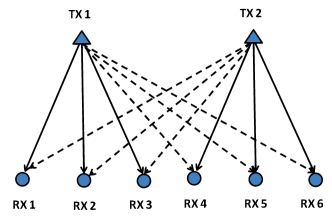
Figure 5: The cellular network model considered in Section VIII-A. The solid lines represent the direct channels, while the dotted lines represent the interfering channels.

When linear transceivers are used at the base stations and the users, user $i_{k}$’s received signal vector, denoted as $\mathbf{y}_{i_{k}}\in\mathbb{C}^{N}$, can be written as

$$\mathbf{y}_{i_{k}} =\underbrace{{\mathbf{H}}_{i_{k}k}{\textbf{V}}_{i_{k}}\mathbf{s}_{i_{k}}}_{\textrm{desired signal}}+\underbrace{\sum_{\ell\neq i,\ell=1}^{I_{k}}{\mathbf{H}}_{i_{k}k}{\textbf{V}}_{\ell_{k}}\mathbf{s}_{\ell_{k}}}_{\textrm{intracell interference}}+\underbrace{\sum_{j\neq k,j=1}^{K}\sum_{\ell=1}^{I_{j}}{\mathbf{H}}_{i_{k}j}{\textbf{V}}_{\ell_{j}}\mathbf{s}_{\ell_{j}}+\mathbf{n}_{i_{k}}}_{\textrm{intercell interference plus noise}},\;\forall\;i_{k}\in\mathcal{I},$$

where ${\textbf{V}}_{i_{k}}\in\mathbb{C}^{M\times d_{i_{k}}}$ is the linear transmit beamformer used by base station $k$ for user $i_{k}$; $\mathbf{s}_{i_{k}}\in\mathbb{C}^{d_{i_{k}}\times 1}$ is user $i_{k}$’s data signal. The matrix ${\mathbf{H}}_{i_{k}j}$ represents the channel from transmitter $j$ to receiver $i_{k}$, and $\mathbf{n}_{i_{k}}$ denotes the complex additive white Gaussian noise with distribution $\mathcal{CN}(0,\sigma_{i_{k}}^{2}\mathbf{I})$. User $i_{k}$ estimates the intended message using a linear beamformer  $\mathbf{U}_{i_{k}}\in\mathbb{C}^{M\times d_{i_{k}}}$: $\hat{\mathbf{s}}_{i_{k}}=\mathbf{U}^{H}_{i_{k}}\mathbf{y}_{i_{k}}.$

Treating interference as noise, the rate of user $i_{k}$ is given by

$$R_{i_{k}}({\textbf{V}}) =\log\det\bigg{(}\mathbf{I}+{\mathbf{H}}_{i_{k}k}{\textbf{V}}_{i_{k}}({\textbf{V}}_{i_{k}})^{H}{\mathbf{H}}_{i_{k}k}^{H}\bigg{(}\sigma_{i_{k}}^{2}\mathbf{I}+\sum_{(j,\ell)\neq(k,i)}{\mathbf{H}}_{i_{k}j}{\textbf{V}}_{\ell_{j}}({\textbf{V}}_{\ell_{j}})^{H}{\mathbf{H}}_{i_{k}j}^{H}\bigg{)}^{-1}\bigg{)}.$$

We are interested in finding the beamformers V such that the sum of the users’ rates are optimized

$$\begin{split}\max_{\{{\textbf{V}}_{i_{k}}\}_{i_{k}\in\mathcal{I}}}\quad&\sum_{k=1}^{K}\sum_{i=1}^{I_{k}}R_{i_{k}}({\textbf{V}})\\ \textrm{s.t.}\quad&\sum_{i=1}^{I_{k}}{\rm Tr}({\textbf{V}}_{i_{k}}{\textbf{V}}_{i_{k}}^{H})\leq\bar{P}_{k},\;\;\forall\;k\in\mathcal{K}.\end{split}$$ (40)

Note that we have included a transmit power constraint for each base station. It has been shown in [20] that solving (40) is NP-hard. Therefore, we try to obtain the stationary solution for this problem. Furthermore, we can no longer straightforwardly apply the BSUM algorithm that updates ${\textbf{V}}_{i_{k}}$’s cyclically. This is due to the fact that the users in the set $\mathcal{I}_{k}$ share a common power constraint. Thus the requirement for the separability of the constraints for different block components in (12) is not satisfied.

To devise an efficient and low complexity algorithm for problem (40), we will first transform this problem to a more suitable form. We first introduce the function $f_{i_{k}}(\mathbf{U}_{i_{k}},{\textbf{V}})\triangleq\log\det\left(\mathbf{E}_{i_{k}}^{-1}\right)$, where $\mathbf{E}_{i_{k}}$ is the mean square error (MSE) matrix given as

$$\begin{split}\mathbf{E}_{i_{k}}\triangleq(\mathbf{I}-\mathbf{U}_{i_{k}}^{H}{\mathbf{H}}_{i_{k}k}{\textbf{V}}_{i_{k}})(\mathbf{I}-\mathbf{U}_{i_{k}}^{H}{\mathbf{H}}_{i_{k}k}{\textbf{V}}_{i_{k}})^{H}+\sum_{(\ell,j)\neq(i,k)}\mathbf{U}_{i_{k}}^{H}{\mathbf{H}}_{i_{k}j}{\textbf{V}}_{\ell_{j}}{\textbf{V}}_{\ell_{j}}^{H}{\mathbf{H}}_{i_{k}j}^{H}\mathbf{U}_{i_{k}}+\sigma_{i_{k}}^{2}\mathbf{U}_{i_{k}}^{H}\mathbf{U}_{i_{k}}.\end{split}$$

In the subsequent presentation we will occasionally use the notation $\mathbf{E}_{i_{k}}(\mathbf{U}_{i_{k}},{\textbf{V}})$ to make the dependency of the MSE matrix and the transceivers explicit.

Taking the derivative of $f_{i_{k}}(\mathbf{U}_{i_{k}},{\textbf{V}})$ with respect to $\mathbf{U}_{i_{k}}$ and checking the first order optimality condition, we have

$$\arg\max_{\mathbf{U}_{i_{k}}}f_{i_{k}}(\mathbf{U}_{i_{k}},{\textbf{V}})=\bigg{(}\sigma_{i_{k}}^{2}\mathbf{I}+\sum_{(j,\ell)}{\mathbf{H}}_{i_{k}j}{\textbf{V}}_{\ell_{j}}{\textbf{V}}_{\ell_{j}}^{H}{\mathbf{H}}_{i_{k}j}^{H}\bigg{)}^{-1}{\mathbf{H}}_{i_{k}k}.{\textbf{V}}_{i_{k}}$$

Plugging in the optimal value of $\mathbf{U}_{i_{k}}$ in $f_{i_{k}}(\cdot)$, we obtain $\max_{\mathbf{U}_{i_{k}}}~{}f_{i_{k}}(\mathbf{U}_{i_{k}},{\textbf{V}})=R_{i_{k}}({\textbf{V}}).$ Thus, we can rewrite the optimization problem equivalently (40) as

$$\begin{split}\min_{{\textbf{V}},\mathbf{U}}\quad&\sum_{k=1}^{K}\sum_{i=1}^{I_{k}}\log\det(\mathbf{E}_{i_{k}})\\ {\rm s.t.}\quad&\sum_{i=1}^{I_{k}}{\rm Tr}\,({\textbf{V}}_{i_{k}}{\textbf{V}}_{i_{k}}^{H})\leq P_{k},\,\,\forall\;k\in\mathcal{K}.\end{split}$$ (41)

Notice the fact that the function $\log\det(\cdot)$ is a concave function on its argument (see, e.g., [5]), then for any feasible $\mathbf{E}_{i_{k}}$, $\widehat{\mathbf{E}}_{i_{k}}$, we have

$$\log\det(\mathbf{E}_{i_{k}}) \leq\log\det(\widehat{\mathbf{E}}_{i_{k}})+{\rm Tr}[\triangledown_{\mathbf{E}_{i_{k}}}(\log\det(\widehat{\mathbf{E}}_{i_{k}}))(\mathbf{E}_{i_{k}}-\widehat{\mathbf{E}}_{i_{k}})]$$

$$=\log\det(\widehat{\mathbf{E}}_{i_{k}})+{\rm Tr}[\widehat{\mathbf{E}}^{-1}_{i_{k}}(\mathbf{E}_{i_{k}}-\widehat{\mathbf{E}}_{i_{k}})]\triangleq u_{i_{k}}(\mathbf{E}_{i_{k}},\widehat{\mathbf{E}}_{i_{k}})$$ (42)

Utilizing the above transformation and the upper bound, we can again apply the BSUM algorithm. Let V and $\mathbf{U}$ be two block variables. Define

$$u_{{\textbf{v}}}\left({\textbf{V}},(\widehat{{\textbf{V}}},\widehat{\mathbf{U}})\right) \triangleq\sum_{k=1}^{K}\sum_{i=1}^{I_{k}}u_{i_{k}}(\mathbf{E}_{i_{k}}({\textbf{V}},\widehat{\mathbf{U}}_{i_{k}}),{\mathbf{E}}_{i_{k}}(\widehat{{\textbf{V}}},\widehat{\mathbf{U}}_{i_{k}}))$$

$$u_{\mathbf{u}}\left(\mathbf{U},(\widehat{{\textbf{V}}},\widehat{\mathbf{U}})\right) \triangleq\sum_{k=1}^{K}\sum_{i=1}^{I_{k}}u_{i_{k}}(\mathbf{E}_{i_{k}}(\widehat{{\textbf{V}}},\mathbf{U}_{i_{k}}),{\mathbf{E}}(\widehat{{\textbf{V}}},\widehat{\mathbf{U}}_{i_{k}}))$$

In iteration $2r+1$, the algorithm solves the following problem

$$\begin{split}\min_{{\textbf{V}}}&\quad u_{\textbf{v}}\left({\textbf{V}},({\textbf{V}}^{2r},\mathbf{U}^{2r})\right)\\ &\quad\sum_{i=1}^{I_{k}}{\rm Tr}\,({\textbf{V}}_{i_{k}}{\textbf{V}}_{i_{k}}^{H})\leq P_{k},\,\,\forall\;k\in\mathcal{K}.\end{split}$$ (43)

In iteration $2r+2$, the algorithm solves the following (unconstrained) problem

$$\begin{split}\min_{\mathbf{U}}\quad&u_{\mathbf{u}}\left(\mathbf{U},({\textbf{V}}^{2r+1},\mathbf{U}^{2r})\right)\end{split}$$ (44)

The above BSUM algorithm for solving (40) is called WMMSE algorithm in the reference [28].

Due to (42), we must have that

$$u_{\textbf{v}}\left({\textbf{V}},({\textbf{V}}^{2r},\mathbf{U}^{2r})\right)\geq\sum_{k=1}^{K}\sum_{i=1}^{I_{k}}\log\det(\mathbf{E}_{i_{k}}({\textbf{V}},\mathbf{U}^{2r}_{i_{k}})),\quad{\rm for~{}all~{}feasible~{}}{\textbf{V}},~{}\forall~{}i_{k}$$

$$u_{\mathbf{u}}\left(\mathbf{U},({\textbf{V}}^{2r+1},\mathbf{U}^{2r})\right)\geq\sum_{k=1}^{K}\sum_{i=1}^{I_{k}}\log\det(\mathbf{E}_{i_{k}}({\textbf{V}}^{2r+1},\mathbf{U}_{i_{k}}))\quad{\rm for~{}all~{}}\mathbf{U}_{i_{k}},~{}\forall~{}i_{k}$$

Moreover, other conditions in Assumption 2 are also satisfied for $u_{{\textbf{v}}}(\cdot)$ and $u_{\mathbf{u}}(\cdot)$. Thus the convergence of the WMMSE algorithm to a stationary solution of problem (41) follows directly from Theorem 2.

We briefly mention here that the main benefit of using the BSUM approach for solving problem (41) is that in each step, the problem (43) can be decomposed into $K$ independent convex subproblems, one for each base station $k\in\mathcal{K}$. Moreover, the solutions for these $K$ subproblems can be simply obtained in closed form (subject to an efficient bisection search). For more details on this algorithm, we refer the readers to [28] and [25].

The BSUM approach has been extensively used for resource allocation in wireless networks, for example [18, 8, 27, 23, 16], and [26]. However, the convergence of most of the algorithms was not rigorously established.

VIII-B Proximal Minimization Algorithm

The classical proximal minimization algorithm (see, e.g., [3, Section 3.4.3]) obtains a solution of the problem $\min_{\mathbf{x}\in\mathcal{X}}f(\mathbf{x})$ by solving an equivalent problem

$$\min_{\mathbf{x}\in\mathcal{X},\mathbf{y}\in\mathcal{X}}f(\mathbf{x})+\frac{1}{2c}\|\mathbf{x}-\mathbf{y}\|_{2}^{2},$$ (45)

where $f(\cdot)$ is a convex function, $\mathcal{X}$ is a closed convex set, and $c>0$ is a scalar parameter. The equivalent problem (45) is attractive in that it is strongly convex in both $x$ and $y$ (but not jointly) so long as $f(x)$ is convex. This problem can be solved by performing the following two steps in an alternating fashion

$$\mathbf{x}^{r+1} =\arg\min_{\mathbf{x}\in\mathcal{X}}\left\{f(x)+\frac{1}{2c}\|\mathbf{x}-\mathbf{y}^{r}\|^{2}_{2}\right\}$$ (46)

$$\mathbf{y}^{r+1} =\mathbf{x}^{r+1}.$$ (47)

Equivalently, let $u(\mathbf{x};\mathbf{x}^{r})\triangleq f(\mathbf{x})+\frac{1}{2c}\|\mathbf{x}-\mathbf{x}^{r}\|_{2}^{2}$, then the iteration (46)–(47) can be written as

$$\mathbf{x}^{r+1}=\arg\min_{\mathbf{x}\in\mathcal{X}}u(\mathbf{x},\mathbf{x}^{r}).$$ (48)

It can be straightforwardly checked that for all $\mathbf{x},\mathbf{x}^{r}\in\mathcal{X}$, the function $u(\mathbf{x},\mathbf{x}^{r})$ serves as an upper bound for the function $f(\mathbf{x})$. Moreover, the conditions listed in Assumption 1 are all satisfied. Clearly, the iteration (48) corresponds to the SUM algorithm discussed in Section III. Consequently, the convergence of the proximal minimization procedure can be obtained from Theorem 1.

The proximal minimization algorithm can be generalized in the following way. Consider the problem

$$\min_{\mathbf{x}} \quad f(\mathbf{x}_{1},\cdots,\mathbf{x}_{n})$$ (49)

$${\rm s.t.} \quad\mathbf{x}_{i}\in\mathcal{X}_{i},~{}i=1,\cdots,n,$$

where $\{\mathcal{X}_{i}\}_{i=1}^{n}$ are closed convex sets, $f(\cdot)$ is convex in each of its block components, but not necessarily strictly convex. A straightforward application of the BCD procedure may fail to find a stationary solution for this problem, as the per-block subproblems may contain multiple solutions. Alternatively, we can consider an alternating proximal minimization algorithm [12], in each iteration of which the following subproblem is solved

$$\min_{\mathbf{x}_{i}} \quad f(\mathbf{x}^{r}_{1},\ldots,\mathbf{x}_{i-1}^{r},\mathbf{x}_{i},\mathbf{x}_{i+1}^{r},\ldots,\mathbf{x}^{r}_{n})+\frac{1}{2c}\|\mathbf{x}_{i}-\mathbf{x}^{r}_{i}\|^{2}_{2}$$ (50)

$${\rm s.t.} \quad\mathbf{x}_{i}\in\mathcal{X}_{i}.$$

It is not hard to see that this subproblem always admits a unique solution, as the objective is a strictly convex function of $\mathbf{x}_{i}$. Let $u_{i}(\mathbf{x}_{i},\mathbf{x}^{r})\triangleq f(\mathbf{x}^{r}_{1},\cdots,\mathbf{x}_{i},\cdots\mathbf{x}^{r}_{n})+\frac{1}{2c}\|\mathbf{x}_{i}-\mathbf{x}^{r}_{i}\|^{2}_{2}$. Again for each $\mathbf{x}_{i}\in\mathcal{X}_{i}$ and $\mathbf{x}^{r}\in\mathcal{\prod}_{j}\mathcal{X}_{j}$, the function $u_{i}(\mathbf{x}_{i},\mathbf{x}^{r})$ is an upper bound of the original objective $f(\mathbf{x})$. Moreover, all the conditions in Assumption 2 are satisfied. Utilizing Theorem 2, we conclude that the alternating proximal minimization algorithm must converge to a stationary solution of the problem (49). Moreover, our result extends those in [12] to the case of nonsmooth objective function as well as the case with iteration-dependent coefficient $c$. The latter case, which was also studied in the contemporary work [32], will be demonstrated in an example for tensor decomposition shortly.

VIII-C Proximal Splitting Algorithm

The proximal splitting algorithm (see, e.g., [9]) for nonsmooth optimization is also a special case of the BSUM algorithm. Consider the following problem

$$\min_{\mathbf{x}\in\mathcal{X}}f_{1}(\mathbf{x})+f_{2}(\mathbf{x})$$ (51)

where $\mathcal{X}$ is a closed and convex set. Furthermore, $f_{1}$ is convex and lower semicontinuous; $f_{2}$ is convex and has Lipschitz continuous gradient, i.e., $\|\nabla f_{2}(\mathbf{x})-\nabla f_{2}(\mathbf{y})\|\leq\beta\|\mathbf{x}-\mathbf{y}\|$, $\forall~{}\mathbf{x},\mathbf{y}\in\mathcal{X}$ and for some $\beta>0$.

Define the proximity operator ${\rm prox}_{f_{i}}:\mathcal{X}\to\mathcal{X}$ as

$${\rm prox}_{f_{i}}(\mathbf{x})=\arg\min_{\mathbf{y}\in\mathcal{X}}f_{i}(\mathbf{y})+\frac{1}{2}\|\mathbf{x}-\mathbf{y}\|^{2}.$$ (52)

The following forward-backward splitting iteration can be used to obtain a solution for problem (51) [9]:

$$\mathbf{x}^{r+1}=\underbrace{{\rm prox}_{\gamma f_{1}}}_{\rm backward~{}step}\underbrace{(\mathbf{x}^{r}-\gamma\nabla f_{2}(\mathbf{x}^{r}))}_{\rm forward~{}step}$$ (53)

where $\gamma\in[\epsilon,2/\beta-\epsilon]$ with $\epsilon\in]0,\min\{1,1/\beta\}[$. Define

$$u(\mathbf{x},\mathbf{x}^{r})\triangleq f_{1}(\mathbf{x})+\frac{1}{2\gamma}\|\mathbf{x}-\mathbf{x}^{r}\|^{2}+\langle\mathbf{x}-\mathbf{x}^{r},\nabla f_{2}(\mathbf{x}^{r})\rangle+f_{2}(\mathbf{x}^{r}).$$ (54)

We first show that the iteration (53) is equivalent to the following iteration

$$\mathbf{x}^{r+1}=\arg\min_{\mathbf{x}\in\mathcal{X}}u(\mathbf{x},\mathbf{x}^{r}).$$ (55)

From the definition of the prox operation, we have

$${\rm prox}_{\gamma f_{1}}(\mathbf{x}^{r}-\gamma\nabla f_{2}(\mathbf{x}^{r})) =\arg\min_{\mathbf{x}\in\mathcal{X}}\gamma f_{1}(\mathbf{x})+\frac{1}{2}\|\mathbf{x}-\mathbf{x}^{r}+\gamma\nabla f_{2}(\mathbf{x}^{r})\|^{2}_{2}$$

$$=\arg\min_{\mathbf{x}\in\mathcal{X}}f_{1}(\mathbf{x})+\frac{1}{2\gamma}\|\mathbf{x}-\mathbf{x}^{r}\|_{2}^{2}+\langle\mathbf{x}-\mathbf{x}^{r},\nabla f_{2}(\mathbf{x}^{r})\rangle$$

$$=\arg\min_{\mathbf{x}\in\mathcal{X}}u(\mathbf{x},\mathbf{x}^{r}).$$

We then show that $u(\mathbf{x},\mathbf{x}^{r})$ is an upper bound of the original function $f_{1}(\mathbf{x})+f_{2}(\mathbf{x})$, for all $\mathbf{x},\mathbf{x}^{r}\in\mathcal{X}$. Note that from the well known Descent Lemma [2, Proposition A.32], we have that

$$f_{2}(\mathbf{x}) \leq f_{2}(\mathbf{x}^{r})+\frac{\beta}{2}\|\mathbf{x}-\mathbf{x}^{r}\|^{2}+\langle\mathbf{x}-\mathbf{x}^{r},\nabla f_{2}(\mathbf{x}^{r})\rangle$$

$$\leq f_{2}(\mathbf{x}^{r})+\frac{1}{2\gamma}\|\mathbf{x}-\mathbf{x}^{r}\|^{2}+\langle\mathbf{x}-\mathbf{x}^{r},\nabla f_{2}(\mathbf{x}^{r})\rangle$$

where the second inequality is from the definition of $\gamma$. This result implies that $u(\mathbf{x},\mathbf{y})\geq f_{1}(\mathbf{x})+f_{2}(\mathbf{x}),~{}\forall~{}\mathbf{x},\mathbf{y}\in\mathcal{X}$. Moreover, we can again verify that all the other conditions in Assumption 1 is true. Consequently, we conclude that the forward-backward splitting algorithm is a special case of the SUM algorithm.

Similar to the previous example, we can generalize the forward-backward splitting algorithm to the problem with multiple block components. Consider the following problem

$$\min \quad\sum_{i=1}^{n}f_{i}(\mathbf{x}_{i})+f_{n+1}(\mathbf{x}_{1},\cdots,\mathbf{x}_{n})$$ (56)

$${\rm s.t.} \quad\mathbf{x}_{i}\in\mathcal{X}_{i},i=1,\cdots,n$$

where $\{\mathcal{X}_{i}\}_{i=1}^{n}$ are a closed and convex sets. Each function $f_{i}(\cdot)$, $i=1,\cdots n$ is convex and lower semicontinuous w.r.t. $\mathbf{x}_{i}$; $f_{n+1}(\cdot)$ is convex and has Lipschitz continuous gradient w.r.t. each of the component $\mathbf{x}_{i}$, i.e., $\|\nabla f_{n+1}(\mathbf{x})-\nabla f_{n+1}(\mathbf{y})\|\leq\beta_{i}\|\mathbf{x}_{i}-\mathbf{y}_{i}\|$, $\forall~{}\mathbf{x}_{i},\mathbf{y}_{i}\in\mathcal{X}_{i},i=1,\cdots,n$. Then the following block forward-backward splitting algorithm can be shown as a special case of the BSUM algorithm, and consequently converges to a stationary solution of the problem (56)

$$\mathbf{x}_{i}^{r+1}={{\rm prox}_{\gamma f_{i}}}{(\mathbf{x}_{i}^{r}-\gamma\nabla_{\mathbf{x}_{i}}f_{n+1}(\mathbf{x}^{r}))},\quad i=1,2,...,n,$$

where $\gamma\in[\epsilon_{i},2/\beta_{i}-\epsilon_{i}]$ with $\epsilon_{i}\in]0,\min\{1,1/\beta_{i}\}[$.

VIII-D CANDECOMP/PARAFAC Decomposition of Tensors

Another application of the proposed method is in CANDECOMP/PARAFAC (CP) decomposition of tensors. Given a tensor $\mathfrak{X}\in\mathbb{R}^{m_{1}\times m_{2}\times\ldots\times m_{n}}$ of order $n$, the idea of CP decomposition is to write the tensor as the sum of rank-one tensors:

$$\mathfrak{X}=\sum_{r=1}^{R}\mathfrak{X}_{r},$$

where $\mathfrak{X}_{r}=a_{1r}\circ a_{2r}\circ\ldots\circ a_{nr}$ and $a_{ir}\in\mathbb{R}^{m_{i}}$. Here the notation $``\circ"$ denotes the outer product.

In general, finding the CP decomposition of a given tensor is NP-hard [15]. In practice, one of the most widely accepted algorithms for computing the CP decomposition of a tensor is the Alternating Least Squares (ALS) algorithm [19, 11, 29]. The ALS algorithm proposed in [6, 13] is in essence a BCD method. For ease of presentation, we will present the ALS algorithm only for tensors of order three.

Let $\mathfrak{X}\in\mathbb{R}^{I\times J\times K}$ be a third order tensor. Let $(A;B;C)$ represent the following decomposition

$$(A;B;C)\triangleq\sum_{r=1}^{R}a_{r}\circ b_{r}\circ c_{r},$$

where $a_{r}$ (resp. $b_{r}$ and $c_{r}$) is the $r$-th column of $A$ (resp. $B$ and $C$). The ALS algorithm minimizes the difference between the original and the reconstructed tensors

$$\min_{A,B,C}\quad\|\mathfrak{X}-(A;B;C)\|,$$ (57)

where $A\in\mathbb{R}^{I\times R}$, $B\in\mathbb{R}^{J\times R}$, $C\in\mathbb{R}^{K\times R}$, and $R$ is the rank of the tensor.

The ALS approach is a special case of the BCD algorithm in which the three blocks of variables $A,B,$ and $C$ are cyclically updated. In each step of the computation when two blocks of variables are held fixed, the subproblem becomes the quadratic least squares problem and admits closed form updates (see [19]).

One of the well-known drawbacks of the ALS algorithm is the swamp effect where the objective value remains almost constant for many iterations before starting to decrease again. Navasca et al. in [22] observed that adding a proximal term in the algorithm could help reducing the swamp effect. More specifically, at each iteration $r$ the algorithm proposed in [22] solves the following problem for updating the variables:

$$\|\mathfrak{X}-(A;B;C)\|^{2}+\lambda\|A-A^{r}\|^{2}+\lambda\|B-B^{r}\|^{2}+\lambda\|C-C^{r}\|^{2},$$ (58)

where $\lambda\in\mathbb{R}$ is a positive constant. As discussed before, this proximal term has been considered in different optimization contexts and its convergence has been already showed in [12]. An interesting numerical observation in [22] is that decreasing the value of $\lambda$ during the algorithm can noticeably improve the convergence of the algorithm. Such iterative decrease of $\lambda$ can be accomplished in a number of different ways. Our numerical experiments show that the following simple approach to update $\lambda$ can significantly improve the convergence of the ALS algorithm and substantially reduce the swamp effect:

$$\lambda^{r}=\lambda_{0}+\lambda_{1}\frac{\|\mathfrak{X}-(A^{r};B^{r};C^{r})\|}{\|\mathfrak{X}\|},$$ (59)

where $\lambda^{r}$ is the proximal coefficient $\lambda$ at iteration $r$. Theorem 2 implies the convergence is guaranteed even with this update rule of $\lambda$, whereas the convergence result of [12] does not apply in this case since the proximal coefficient is changing during the iterations.

Figure 6 shows the performance of different algorithms for the example given in [22] where the tensor $\mathfrak{X}$ is obtained from the decomposition

$$A=\left[\begin{array}[]{ccc}1&\cos\theta&0\\ 0&\sin\theta&1\\ \end{array}\right],\quad B=\left[\begin{array}[]{ccc}3&\sqrt{2}\cos\theta&0\\ 0&\sin\theta&1\\ 0&\sin\theta&0\\ \end{array}\right],\quad C=\left[\begin{array}[]{ccc}1&0&0\\ 0&1&0\\ 0&0&1\\ \end{array}\right].$$

The vertical axis is the value of the objective function where the horizontal axis is the iteration number. In this plot, ALS is the classical alternating least squares algorithm. The curve for Constant Proximal shows the performance of the BSUM algorithm when we use the objective function in (58) with $\lambda=0.1$. The curve for Diminishing Proximal shows the performance of block coordinate descent method on (58) where the weight $\lambda$ decreases iteratively according to (59) with $\lambda_{0}=10^{-7},\lambda_{1}=0.1$. The other two curves MBI and MISUM correspond to the maximum block improvement algorithm and the MISUM algorithm. In the implementation of the MISUM algorithm, the proximal term is of the form in (58) and the weight $\lambda$ is updated based on (59).

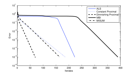
Figure 6: Convergence of Different Algorithms

Table I represents the average number of iterations required to get an objective value less than $\epsilon=10^{-5}$ for different algorithms. The average is taken over 1000 Monte-Carlo runs over different initializations. The initial points are generated randomly where the components of the variables $A,B,$ and $C$ are drawn independently from the uniform distribution over the unit interval $[0,1]$. As it can be seen, adding a diminishing proximal term significantly improves the convergence speed of the ALS algorithm.

Algorithm	Average number of iterations for convergence
ALS	277
Constant Proximal	140
Diminishing Proximal	78
MBI	572
MISUM	175

TABLE I: Average number of iterations for convergence

VIII-E Expectation Maximization Algorithm

The expectation maximization algorithm (EM) in [10] is an iterative procedure for maximum likelihood estimation when some of the random variables are unobserved/hidden. Let $w$ be the observed random vector which is used for estimating the value of $\theta$. The maximum likelihood estimate of $\theta$ can be given as

$$\hat{\theta}_{\rm ML}=\arg\max_{\theta}\;\ln p(w|\theta).$$ (60)

Let the random vector $z$ be the hidden/unobserved variable. The EM algorithm starts from an initial estimate $\theta^{0}$ and generates a sequence $\{\theta^{r}\}$ by repeating the following steps:

• E-Step: Calculate $g(\theta,\theta^{r})\triangleq\mathbb{E}_{z|w,\theta^{r}}\{\ln p(w,z|\theta)\}$

• M-Step: $\theta^{r+1}=\arg\max_{\theta}\;g(\theta,\theta^{r})$

The EM-algorithm can be viewed as a special case of SUM algorithm [4]. In fact, we are interested in solving the following optimization problem

$$\min_{\theta}\quad-\ln p(w|\theta).$$

The objective function could be written as

$$-\ln p(w|\theta) =-\ln\;\;\mathbb{E}_{z|\theta}\;p(w|z,\theta)$$

$$=-\ln\;\;\mathbb{E}_{z|\theta}\left[\frac{p(z|w,\theta^{r})p(w|z,\theta)}{p(z|w,\theta^{r})}\right]$$

$$=-\ln\;\;\mathbb{E}_{z|w,\theta^{r}}\left[\frac{p(z|\theta)p(w|z,\theta)}{p(z|w,\theta^{r})}\right]$$

$$\leq-\mathbb{E}_{z|w,\theta^{r}}\ln\left[\frac{p(z|\theta)p(w|z,\theta)}{p(z|w,\theta^{r})}\right]$$

$$=-\mathbb{E}_{z|w,\theta^{r}}\ln p(w,z|\theta)+\mathbb{E}_{z|w,\theta^{r}}\ln p(z|w,\theta^{r})$$

$$\triangleq u(\theta,\theta^{r}),$$

where the inequality is due to the Jensen’s inequality and the third equality follows from a simple change of the order of integration for the expectation. Since $\mathbb{E}_{z|w,\theta^{r}}\ln p(z|w,\theta^{r})$ is not a function of $\theta$, the M-step in the EM-algorithm can be written as

$$\theta^{r+1}=\arg\max_{\theta}u(\theta,\theta^{r}).$$

Furthermore, it is not hard to see that $u(\theta^{r},\theta^{r})=-\ln p(w|\theta^{r})$. Therefore, under the smoothness assumption, Proposition 1 implies that Assumption 1 is satisfied. As an immediate consequence, the EM-algorithm is a special case of the SUM algorithm. Therefore, our result implies not only the convergence of the EM-algorithm, but also the convergence of the EM-algorithm with Gauss-Seidel/coordinatewise update rule (under the assumptions of Theorem 2). In fact in the block coordinate EM-algorithm (BEM), at each M-step, only one block is updated. More specifically, let $\theta=(\theta_{1},\ldots,\theta_{n})$ be the unknown parameter. Assume $w$ is the observed vector and $z$ is the hidden/unobserved variable as before. The BEM algorithm starts from an initial point $\theta^{0}=(\theta^{0}_{1},\ldots,\theta^{0}_{n})$ and generates a sequence $\{\theta^{r}\}$ according to the algorithm in Figure 7.

1 Initialize with $\theta^{0}$ and set $r=0$ 2 repeat 3 $r=r+1$, $i=r\;{\rm mod}\;n+1$ 4 E-Step: $g_{i}(\theta_{i},\theta^{r})=\mathbb{E}_{z|w,\theta^{r}}\{\ln p(w,z|\theta_{1}^{r},\ldots,\theta_{i-1}^{r},\theta_{i},\theta_{i+1}^{r},\ldots,\theta_{n}^{r})\}$ 5 M-Step: $\theta_{i}^{r+1}=\arg\max_{\theta_{i}}\;g_{i}(\theta_{i},\theta^{r})$ 6 until some convergence criterion is met

Figure 7: Pseudo code of the BEM algorithm

The motivation behind using the BEM algorithm instead of the EM algorithm could be the difficulties in solving the M-step of EM for the entire set of variables, while solving the same problem per block of variables is easy. To the best of our knowledge, the BEM algorithm and its convergence behavior have not been analyzed before.

VIII-F Concave-Convex Procedure/Difference of Convex Functions

A popular algorithm for solving unconstrained problems, which also belongs to the class of successive upper-bound minimization, is the Concave-Convex Procedure (CCCP) introduced in [33]. In CCCP, also known as the difference of convex functions (DC) programming, we consider the unconstrained problem

$$\min_{x\in\mathbb{R}^{m}}\;f(x),$$

where $f(x)=f_{cve}(x)+f_{cvx}(x),\forall\;x\in\mathbb{R}^{m}$; where $f_{cve}(\cdot)$ is a concave function and $f_{cvx}(\cdot)$ is convex. The CCCP generates a sequence $\{x^{r}\}$ by solving the following equation:

$$\nabla f_{cvx}(x^{r+1})=-\nabla f_{cve}(x^{r}),$$

which is equivalent to

$$x^{r+1}=\arg\min_{x}\;g(x,x^{r}),$$ (61)

where $g(x,x^{r})\triangleq f_{cvx}(x)+(x-x^{r})^{T}\nabla f_{cve}(x^{r})+f_{cve}(x^{r})$. Clearly, $g(x,x^{r})$ is a tight convex upper-bound of $f(x)$ and hence CCCP is a special case of the SUM algorithm and its convergence is guaranteed by Theorem 1 under certain assumptions. Furthermore, if the updates are done in a block coordinate manner, the algorithm becomes a special case of BSUM whose convergence is guaranteed by Theorem 2. To the best of our knowledge, the block coordinate version of CCCP algorithm and its convergence has not been studied before.

References

• [1] Z. L. B. Chen, Simai He and S. Zhang, “Maximum block improvement and polynomial optimization,” SIAM Journal on Optimization, vol. 22, pp. 87–107, 2012.
• [2] D. P. Bertsekas, Nonlinear Programming, 2nd ed.   Athena-Scientific, 1999.
• [3] D. P. Bertsekas and J. N. Tsitsiklis, Parallel and Distributed Computation: Numerical Methods, 2nd ed.   Athena-Scientific, 1999.
• [4] S. Borman, “The expectation maximization algorithm - a short tutorial,” Unpublished paper. [Online]. Available: http://ftp.csd.uwo.ca/faculty/olga/Courses/Fall2006/Papers/EM_algorithm%.pdf
• [5] S. Boyd and L. Vandenberghe, Convex Optimization.   Cambridge University Press, 2004.
• [6] J. D. Carroll and J. J. Chang, “Analysis of individual differences in multidimensional scaling via an n-way generalization of “Eckart-Young” decomposition,” Psychometrika, vol. 35, pp. 283–319, 1970.
• [7] Y. Censor and S. A. Zenios, Parallel Optimization: Theory, Algorithm, and Applications.   Oxford University Press, Oxford, United Kingdom, 1997.
• [8] M. Chiang, C. W. Tan, D. P. Palomar, D. O’Neill, and D. Julian, “Power control by geometric programming,” IEEE Transactions on Wireless Communications, vol. 6, pp. 2640–2651, 2007.
• [9] P. L. Combettes and J.-C. Pesquet, “Proximal splitting methods in signal processing,” 2009, available online at: arxiv.org.
• [10] A. P. Dempster, N. M. Laird, and D. B. Rubin, “Maximum likelihood from incomplete data via the EM algorithm,” Journal of the Royal Statistical Society Series B, vol. 39, pp. 1–38, 1977.
• [11] N. K. M. Faber, R. Bro, and P. K. Hopke, “Recent developments in CANDECOMP/PARAFAC algorithms: A critical review,” Chemometrics and Intelligent Laboratory Systems, vol. 65, pp. 119–137, 2003.
• [12] L. Grippo and M. Sciandrone, “On the convergence of the block nonlinear Gauss-Seidel method under convex constraints,” Operations Research Letters, vol. 26, pp. 127–136, 2000.
• [13] R. A. Harshman, “Foundations of the parafac procedure: Models and conditions for an explanatory” multi-modal factor analysis,” UCLA working papers in phonetics, vol. 16, pp. 1–84, 1970.
• [14] J. A. Hartigan and M. A. Wong, “K-means clustering algorithm,” Journal of the Royal Statistical Society, Series C (Applied Statistics), vol. 28, pp. 100–108, 1979.
• [15] J. Hastad, “Tensor rank is NP-complete,” Journal of Algorithms, vol. 11, pp. 644–654, 1990.
• [16] M. Hong and Z.-Q. Luo, “Joint linear precoder optimization and base station selection for an uplink mimo network: A game theoretic approach,” in the Proceedings of the IEEE ICASSP, 2012.
• [17] H. R. Howson and N. G. F. Sancho, “A new algorithm for the solution of multistate dynamic programming problems,” Mathematical Programming, vol. 8, pp. 104–116, 1975.
• [18] S. J. Kim and G. B. Giannakis, “Optimal resource allocation for mimo ad-hoc cognitive radio networks,” Proceedings of Allerton Conference on Communication, Control, and Computing, 2008.
• [19] T. G. Kolda and B. W. Bader, “Tensor decompositions and applications,” SIAM Review, vol. 51, pp. 455–500, 2009.
• [20] Z.-Q. Luo and S. Zhang, “Dynamic spectrum management: Complexity and duality,” IEEE Journal of Selected Topics in Signal Processing, vol. 2, no. 1, pp. 57–73, 2008.
• [21] B. R. Marks and G. P. Wright, “A general inner approximation algorithm for nonconvex mathematical programs,” Operations Research, vol. 26, pp. 681–683, 1978.
• [22] C. Navasca, L. D. Lathauwer, and S. Kindermann, “Swamp reducing technique for tensor decomposition,” Proc. 16th European Signal Processing Conference (EUSIPCO), August 2008.
• [23] C. T. K. Ng and H. Huang, “Linear precoding in cooperative MIMO cellular networks with limited coordination clusters,” IEEE Journal on Selected Areas in Communications, vol. 28, no. 9, pp. 1446 –1454, december 2010.
• [24] M. J. D. Powell, “On search directions for minimization algorithms,” Mathematical Programming, vol. 4, pp. 193–201, 1973.
• [25] M. Razaviyayn, H. Baligh, A. Callard, and Z.-Q. Luo, “Joint transceiver design and user grouping in a MIMO interfering broadcast channel,” 45th Annual Conference on Information Sciences and Systems (CISS), pp. 1–6, 2011.
• [26] C. Shi, R. A. Berry, and M. L. Honig, “Local interference pricing for distributed beamforming in MIMO networks,” Proceedings of the 28th IEEE conference on Military communications (MILCOM), pp. 1001–1006, 2009.
• [27] ——, “Monotonic convergence of distributed interference pricing in wireless networks,” in Proceedings of the 2009 IEEE international conference on Symposium on Information Theory - Volume 3, ser. ISIT’09, 2009, pp. 1619–1623.
• [28] Q. Shi, M. Razaviyayn, Z.-Q. Luo, and C. He, “An iteratively weighted mmse approach to distributed sum-utility maximization for a MIMO interfering broadcast channel,” IEEE Transactions on Signal Processing, vol. 59, pp. 4331–4340, 2011.
• [29] G. Tomasi and R. Bro, “A comparison of algorithms for fitting the parafac model,” Computational Statistics and Data Analysis, vol. 50, p. 1700 1734, April 2006.
• [30] P. Tseng, “Convergence of a block coordinate descent method for nondifferentiable minimization,” Journal of Optimization Theory and Applications, vol. 109, pp. 475–494, 2001.
• [31] P. Tseng and S. Yun, “A coordinate gradient descent method for nonsmooth separable minimization,” Mathematical Programming, vol. 117, pp. 387–423, 2009.
• [32] Y. Xu and W. Yin, “A block coordinate descent method for multi-convex optimization with applications to nonnegative tensor factorization and completion,” http://www.caam.rice.edu/$\sim$optimization/BCD/, 2012.
• [33] A. L. Yuille and A. Rangarajan, “The concave-convex procedure,” Neural Computation, vol. 15, pp. 915–936, 2003.
• [34] N. Zadeh, “A note on the cyclic coordinate ascent method,” Management Science, vol. 16, pp. 642–644, 1970.