4, place Jussieu, F-75252 Paris Cedex 05, France
11email: Fabrice.Kordon@lip6.fr, 11email: Maximilien.Colange@lip6.fr, 11email: Lom-Messan.Hillah@lip6.fr, 11email: Emmanuel.Paviot-Adet@lip6.fr, 11email: Yann.Thierry-Mieg@lip6.fr
22institutetext: Centre Universitaire d’Informatique, Université de Genève
7, route de Drize, CH-1227 Carouge, Switzerland
22email: Alban.Linard@unige.ch, 22email: Didier.Buchs@unige.ch
33institutetext: LIPN, CNRS UMR 7030, Université Paris 13
99, av. J-B Clément, 93430 Villetaneuse, France
33email: sami.evangelista@lipn.univ-paris13.fr
44institutetext: IBISC, Université d’Évry Val d’Essonne
22 Boulevard de France, 91037 Évry Cedex France
44email: lfronc@ibisc.univ-evry.fr, 44email: franck.pommereau@ibisc.univ-evry.fr
55institutetext: Universität Rostock, 18051 Rostock, Germany
55email: niels.lohmann@uni-rostock.de, 55email: Wimmel@Informatik.Uni-Oldenburg.de, 55email: karsten.wolf@uni-rostock.de 66institutetext: Brandenburg University of Technology at Cottbus
Postbox 10 13 44, 03013 Cottbus, Germany
66email: rohrch@tu-cottbus.de
[options=-s mcc, intoc, columns=2] (ACTIVITY-LOCAL)ss (AlPiNA)ss (Crocodile)ss (GreatSPN)ss (Helena)ss (ITS-Tools)ss (LoLa-binstore)ss (LoLa-bloom)ss (LoLA)ss (Marcie)ss (Neco)ss (PNXDD)ss (PeTe)ss (Sara)ss (SMART)ss (YASPA)ss (UPPAAL)ss
* * *
Model Checking Contest
@ Petri Nets
Report on the 2012 edition
September 2012
F. Kordon,
A. Linard,
D. Buchs,
M. Colange,
S. Evangelista,
L. Fronc,
L.M. Hillah,
N. Lohmann,
E. Paviot-Adet,
F Pommereau,
C. Rohr,
Y. Thierry-Mieg,
H. Wimmel,
K. Wolf
* * *
Raw Report on the Model Checking Contest
at Petri Nets 2012
Abstract
This article presents the results of the Model Checking Contest held at Petri Nets 2012 in Hambourg. This contest aimed at a fair and experimental evaluation of the performances of model checking techniques applied to Petri nets. This is the second edition after a successful one in 2011 [29].
The participating tools were compared on several examinations (state space generation and evaluation of several types of formulæ – structural, reachability, LTL, CTL) run on a set of common models (Place/Transition and Symmetric Petri nets).
After a short overview of the contest, this paper provides the raw results from the context, model per model and examination per examination.
Keywords: Petri Nets, Model Checking, Contest.
1 Introduction
When verifying by model checking a system with formal methods, such as Petri nets, one may have several questions such as:
“When creating the model of a system, should we use structural analysis or an explicit model checker to debug the model?”
“When verifying the final model of a highly concurrent system, should we use a symmetry-based or a partial order reduction-based model checker?”
“When updating a model with large variable domains, should we use a decision diagram-based or an abstraction-based model checker?”
Results that help to answer these questions are spread among numerous papers in numerous conferences. The choice of the models and tools used in benchmarks is rarely sufficient to answer these questions. Benchmark results are available a long time after their publication, even if the computer architecture has changed a lot. Moreover, as they are executed over several platforms and composed of different models, conclusions are not easy.
The objective of the Model Checking Contest @ Petri nets is to compare the efficiency of verification techniques according to the characteristics of the models. To do so, the Model Checking Contest compares tools on several classes of models with scaling capabilities, e.g., values that set up the “size” of the associated state space.
Through a benchmark, our goal is to identify the techniques that can tackle a given type of problem identified in a “typical model”, for a given class of problem (e.g., state space generation, evaluation of reachability or temporal formulaæ, etc.).
The second edition of the Model Checking Contest @ Petri nets took place within the context of the Petri Nets and ACSD 2012 conferences, in Hamburg, Germany111A First edition took place in Newcastle, UK, withing the context of the SUMo workshop, associated to the Petri Nets et ACSD 2011 conferences [29].. The original submission procedure was published early March 2012 and submissions gathered by mid-May 2012. After some tuning of the execution environment, the evaluation procedure was operated on a cluster early June. Results were presented during the SUMo workshop, on June \nth26, 2012.
The goal of this paper is to report the raw data provided by this second edition of the Model Checking Contest. It reflects the vision of MCC’2012 organizers, as it was first presented in Hamburg. All tool developers are listed in Section 9.
The article is structured as follows. Section 2 presents the models proposed in this second edition. Then, Section 3 lists some information on the participating tools. Section 2 provides an overview of the evaluation methodology. Finally, Sections 5, 6 and 7 present the raw data we collected from MCC’2012.
2 Selected Models
A first innovation in MCC’2012 was to add a “call for model”. The idea was to gather benchmarks from the community. Then, on top of the 7 models proposed in the first edition, we got 12 models from various institutes, usually coming from some tool benchmarks. When models were colored, we requested submitters to provide both the colored version and the Place/Transition (P/T) equivalent version.
The models were provided in PNML format [26, 27]. Tools developers could use the PNML description to build the one of their tool. PNML was then used as the reference. 17 out of the 19 models had scaling parameters. Thus, we could process them with various values and then see how tools could scale up with these models.
We provide below a brief description of models. Moreover, each one has a data-sheet available on MCC’2012 web site: http://mcc.lip6.fr/2012.
2.1 Models from MCC’2011
These first seven models are from the MCC’2011. In this set, MAPK is the only model coming from a case study (biology).
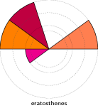
2.1.1 FMS
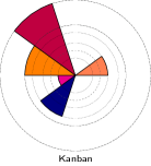
2.1.2 Kanban
[10] models a Kanban system. The scaling parameter corresponds to the number of initial tokens held in four places. The following values were used: .
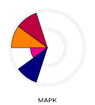
2.1.3 MAPK
models a biological system: the Mitogen-Activated Protein Kinase Kascade [23]. The scaling parameter changes the initial number of tokens held in seven places. The following values were used: .
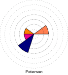
2.1.4 Peterson
models Peterson’s mutual exclusion algorithm [35] in its generalized version for processes. This algorithm is based on shared memory communication and uses a loop with iterations, each iteration is in charge of stopping one of the competing processes. The scaling parameter is the number of involved processes. The following values were used: .
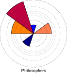
2.1.5 Philosophers
models the famous Dining Philosophers problem introduced by E.W. Dijkstra in 1965 [46] to illustrate an inappropriate use of shared resources, thus generating deadlocks or starvation. The scaling parameter is the number of philosophers. The following values were used: , , , , , , , , , , .
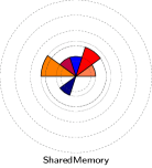
2.1.6 SharedMemory
is a model taken from the GreatSPN benchmarks [8]. It models a system composed of processors competing for the access to a shared memory (built with their local memory) using a unique shared bus. The scaling parameter is the number of processors. The following values were used: .
2.1.7 TokenRing
is another problem proposed by E.W. Dijkstra [18]. It models a system where a set of machines is placed in a ring, numbered to . Each machine only knows its own state and the state of its left neighbor, i.e., machine . Machine number 0 plays a special role, and it is called the “bottom machine”. A protocol ensuring non-starvation determines which machine has a “privilege” (e.g. the right to access a resource). The scaling parameter is the number of machines. The following values were used: .
2.2 New Models in MCC’2012
These twelve models were submitted by the community for MCC’2012. In this new set, several models are coming from larger case studies: neo-election, planning, and ring.
2.2.1 cs_repetitions
models a client/server application with clients and servers. Communication from clients to servers is not reliable, with requests stored in a buffer of size . Communication from servers to clients are reliable. A client send its message until it receives an answer. The scaling parameter is a function of for a fixed number of severs. The following values were used: .
2.2.2 echo
This file specifies the Echo Algorithm (see [38]) for grid like networks. It is a protocol for propagation of information with feedback in a network. A distinguished agent (initiator), starts the distribution of a message by sending it to all its neighbors. On receiving some first message, every other agent forwards the message to all its neighbors, except the one it received its first message from. Then it awaits messages from all recipients of its forwards (regardless whether these messages had been intended as forwards or acknowledgments) and replies to the agent where it received its first message from. As soon as the initiator receives a message from all its neighbors, the protocol terminates. In this example, agents are arranged in a hypercube that can be scaled in two values: , the number of dimensions and , the number of agents per dimensions. The scaling parameter is a combination of and . The following values were used: , , , , , , , , , , .
2.2.3 eratosthenes
This model implements the sieve of Eratosthenes [47]. The scaling parameter is the size of the sieve. The following values were used: .
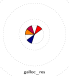
2.2.4 galloc_res
It models the deadlock-free management of mutually exclusive resources known as the “global allocation strategy” [31]. When a process enters a critical section, it locks all the resources needed to be used in the critical section (in the model, 4 max). Then, it can release a subset of these resources (max 2 in the model) at a time (and then stay in the critical section) or exit the critical section, thus releasing all the remaining resources it locks. The scaling parameter is a value for processes and resources. The following values were used: .
2.2.5 lamport_fmea
It models Lamport’s fast mutual exclusion algorithm designed for multi-processor architectures with a shared memory and was studied in [28]. The scaling parameter is the number of processes competing for the critical section. The following values were used: .
2.2.6 neo-election
The Neo protocol aims at managing large distributed databases on clusters of workstations. The machines on the cluster may have several roles. This model focusses on master nodes which handle the communications between all nodes, and in particular requests for accessing database objects. Prior to that all master nodes agree on a primary master which will be the operating one, the other master nodes being secondary, waiting to replace the primary master if needed. This model specifies this election algorithm [9]. The scaling parameter is the number of master nodes. The following values were used: .
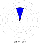
2.2.7 philo_dyn
is a variation of the Dining Philosophers where philosophers can join or quit the table [5]. Each philosopher has its own fork, as in the usual version. The interesting point is that identifiers of left and right for each philosopher must be computed or stored somewhere. A philosopher can enter the table only if the two forks around his position are available. He can leave if his fork is free, and he is thinking. The scaling parameter is the maximum number of philosophers. The following values were used: .
2.2.8 planning
It models the equipment (displays, canvases, documents, and lamps) of a smart conference room of the University of Rostock. It was derived from a proprietary description format that was used by an AI planning tool to generated plans to bring the room in a desired state, for instance displaying a document on a certain canvas while switching off the lights. This problem can be expressed as a reachability problem. This model has no scaling parameter.
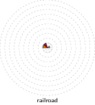
2.2.9 railroad
it corresponds to the Petri nets semantics of an ABCD model of a railroad crossing system. t has three components: a gate sub-net, a controller sub-net and tracks sub-nets that differ only by an identifier in . These components communicate through shared places, some being low-level places to exchange signals, others being integer-valued places to exchange tracks identifiers. The controller also has a place to count the number of trains at a given time. The scaling parameter is the number of tracks. The following values were used: .
2.2.10 ring
It models a three-module ring architecture [17]. The communication architecture contains as many channels as there are modules. It tests the occurrence of global deadlock arising from a local one. It uses stoppable clocking scheme on arbitrated input and output channels. This model has no scaling parameter.
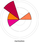
2.2.11 rwmutex
It models a system with readers and writers [38]. Reading can be conducted concurrently whereas writing has to be done exclusively. This is modeled by a number of semaphores (one for each reader) that need to be collected by a writer prior to writing. The scaling parameter a combination of , the number of readers and , the number of writers. The following values were used: , , , , , , , , , , , .
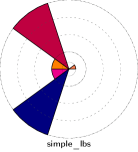
2.2.12 simple_lbs
models a simple load balancing system composed of a set of clients, two servers, and between these, a load balancer process. The scaling parameter is the number of clients to be balanced over the servers. The following values were used: , , , , , , , , , , .
3 Participating Tools
We got 10 tool submissions summarized in Table 1: AlPiNA, Crocodile, Helena, ITS-Tools, LoLa-binstore, LoLa-bloom, Marcie, Neco, PNXDD, and Sara. Their descriptions, written by the tool developers, are given in this section.
| Tool Name | Team | Institution | Country | Contact Name |
| AlPiNA | CUI/SMV | Univ. Geneva | Switzerland | D. Buchs |
| Crocodile | LIP6/MoVe | UPMC | France | M. Colange |
| Helena | LIPN/LCR | Univ. Paris 13 | France | S. Evangelista |
| ITS-Tools | LIP6/MoVe | UPMC | France | Y. Thierry-Mieg |
| LoLA | Team Rostock | Univ. Rostock | Germany | N. Lohmann & K. Wolf |
| Marcie | DSSZ | Univ. Cottbus | Germany | M. Heiner & C. Rohr |
| Neco | IBISC | Univ. Evry | France | L. Fronc |
| PNXDD | LIP6/MoVe | UPMC | France | E. Paviot-Adet |
| Sara | Team Rostock | Univ. Rostock | Germany | H. Wimmel & K. Wolf |
3.0.1 AlPiNA
222Tool is available at http://alpina.unige.ch.[25] stands for Algebraic Petri nets Analyzer and is a symbolic model checker for Algebraic Petri nets. It can verify various state properties expressed in a first order logic property language.
Algebraic Petri nets (APNs) (Petri nets + Abstract Algebraic Data Types) is a powerful formalism to model concurrent systems in a compact way. Usually, concurrent systems have very large sets of states, that grow very fast in relation to the system size. Symbolic Model Checking (DD-based one) is a proven technique to handle the State Space Explosion for simpler formalisms such as Place/Transition nets. AlPiNA extend these concepts to handle algebraic values that can be located in net places.
For this purpose AlPiNA uses enhanced DDs such as Data Decision Diagrams and Set Decision Diagrams for representing the place vectors and Σ Decision Diagrams [3] for representing the values of the APN. It also allows to specify both algebraic and topological clusters to group states together and thus to reduce the memory footprint. Particular care has been taken to let users freely model their systems in APNs and in a second independent step to tune the optimization parameters such as unfolding rules, variable order, and algebraic clustering. Compared to Colored net approaches, AlPiNA [4] solves problems related to the unbounded nature of data types and uses the inductive nature of Abstract Algebraic Data Types to generalize the unfolding and clustering techniques to any kind of data structure.
AlPiNA’s additional goal is to provide a user friendly suite of tools for checking models based on the Algebraic Petri nets formalism. In order to provide great user experience, it leverages the Eclipse platform.
3.0.2 Crocodile
333Tool is available at http://move.lip6.fr/software/Crocodile.[15] was initially designed as a demonstration tool for the so-called symbolic/symbolic approach [43]. It combines two techniques for handling the combinatorial explosion of the state space that are both called “symbolic”.
The first “symbolic” technique concerns the reduction of the reachability graph of a system by its symmetries. The method used in Crocodile was first introduced in [6] for the Symmetric nets, and was then extended to the Symmetric nets with Bags (SNB) in [21]. A symbolic reachability graph (also called quotient graph) can be built for such types of Petri nets, thus dramatically reducing the size of the state space.
The second “symbolic” technique consists in storing the reachability graph using decision diagrams, leading to a symbolic memory encoding. Crocodile relies on Hierarchical Set Decision Diagrams [16]. These present several interesting features, such as hierarchy, and the ability to define inductive operations.
Still under development, Crocodile essentially generates the state space of a SNB and then processes reachability properties. The version submitted for this second edition of the Model Checking Contest includes new strategies for the management of bags [14].
3.0.3 Helena
444Tool is available at http://helena-mc.sourceforge.net.[19] is an explicit state model checker for High Level Petri nets. It is a command-line tool available available under the GNU GPL.
Helena tackles the state explosion problem mostly through a reduction of parallelism operated at two stages of the verification process. First, static reduction rules are applied on the model in order to produce a smaller net that – provided some structural conditions are verified – is equivalent to the original one but has a smaller reachability graph. Second, during the search, partial order reduction is employed to limit, as much as possible, the exploration of redundant paths in the reachability graph. This reduction is based on the detection of independent transitions of the net at a given marking. Other reduction techniques are also implemented by Helena, e.g., state compression, but were disabled during the contest due to their inadequacy with the proposed models.
3.0.4 ITS-Tools
555Tool is available at http://ddd.lip6.fr.[44] are a set of tools to analyze Instantiable Transition Systems, introduced in [44]. This formalism allows compositional specification using a notion of type and instance inspired by component oriented models. The basic elementary types are labeled automata structures, or labeled Petri nets with some classical extensions (inhibitor arcs, reset arcs). The instances are composed using event-based label synchronization.
The main strength of ITS-Tools is that they rely on Hierarchical Set Decision Diagrams [16] to perform analysis. These decision diagrams support hierarchy, allowing to share representation of states for some subsystems. When the system is very regular or symmetric, recursive encodings [44] may even allow to reach logarithmic overall complexity when performing analysis. Within the contest, the Philosophers and TokenRing examples proved to be tractable using this recursive folding feature.
Set Decision Diagrams also offer support for automatically enabling the “saturation” algorithm for symbolic least fixpoint computations [22], a feature allowing to drastically reduce time and memory consumption. This feature was used in all computations.
3.0.5 LoLA
666Tool is available at http://www.informatik.uni-rostock.de/tpp/lola.[49] is an explicit Petri net state space verification tools. It can verify a variety of properties ranging from questions regarding single Petri net nodes (e.g., boundedness of a place or quasiliveness of a transition), reachability of a given state or a state predicate, typical questions related to a whole Petri net (e.g., deadlock freedom, reversibility, or boundedness), and the validity of temporal logical formulae such as CTL. It has been successfully used in case studies from various domains, including asynchronous circuits, biochemical reaction chains, services, business processes, and parameterized Boolean programs.
For each property, LoLA provides tailored versions of state space reduction techniques such as stubborn sets, symmetry reduction, coverability graph generation, or methods involving the Petri net invariant calculus. Depending on the property to be preserved, these techniques can also be used in combination to only generate a small portion of the state space.
Two versions of LoLA were submitted in 2012. LoLa-binstore is a complete reimplementation of the tool since 2011. LoLa-bloom uses a bit hashing technique.
3.0.6 Marcie
777Tool is available at http://www-dssz.informatik.tu-cottbus.de/DSSZ/Software/Marcie.[41] is a tool for the analysis of Generalized Stochastic Petri Nets, supporting qualitative and quantitative analyses including model checking facilities. Particular features are symbolic state space analysis including efficient saturation-based state space generation, evaluation of standard Petri net properties as well as CTL model checking.
Most of Marcie’s features are realized on top of an Interval Decision Diagram implementation [45]. IDDs are used to efficiently encode interval logic functions representing marking sets of bounded Petri nets. This allows to efficiently support qualitative state space based analysis techniques [42]. Further, Marcie applies heuristics for the computation of static variable orders to achieve small decision diagram representations.
For quantitative analysis Marcie implements a multi-threaded on-the-fly computation of the underlying CTMC. It is thus less sensitive to the number of distinct rate values than approaches based on, e.g., Multi-Terminal Decision Diagrams. Further it offers symbolic CSRL model checking and permits to compute reward expectations. Additionally Marcie provides simulative and explicit approximative numerical analysis techniques.
3.0.7 Neco
888Tool is available at http://code.google.com/p/neco-net-compiler/.is a coloured Petri nets compiler which produces libraries for explicit model-checking. These libraries can be used to build state spaces. It is a command-line tool available under the GNU Lesser GPL.
Neco is based on the SNAKES [36] toolkit and handles coloured Petri nets annotated with arbitrary Python [37] objects. This allows for a high degree of expressivity. Extracting information from models, Neco can identify object types and produce optimized Python or C exploration code. The later is done using the Cython [2] language. Moreover, if a part of the model cannot be compiled efficiently a Python fallback is used to handle this part of the model.
Neco also performs model based optimizations using place bounds [20] and control flow places for more efficient firing functions. However, these optimizations are closely related to a modelling language we use which allows them to be assumed by construction. Because the models from the contest were not provided with such properties, these optimizations could not be used.
3.0.8 PNXDD
999Tool is available at https://srcdev.lip6.fr/trac/research/NEOPPOD/wiki/pnxdd.generates the state-space of Place/Transition nets. When Colored nets are used in the Model Checking Contest, equivalent P/Ts are obtained after an “optimized” unfolding [30] (unused places and transitions are detected and suppressed).
State space storage relies on Hierarchical Set Decision Diagrams [16] (SDDs). These are decision diagrams with any data type associated to arcs (see e.g., [33] for an overview of DD-like structures). If the associated data type is another SDD, hierarchical structures can be constructed.
Since PNXDD exploits hierarchy, a state is seen as a tree, where the leaves correspond to places marking. This particular structure offers greater sharing opportunities than a, for instance, vector-based representation. The conception of such a tree is critical to reach good performances and heuristics are being elaborated for this purpose [24]. The one used for the Model Checking Contest is based on [1]: for colored models that do scale via the size of color types, PNXDD uses a tree-like version of this heuristic, while the original version is kept when colored models only scale via the number of tokens in the initial marking.
3.0.9 Sara
101010Tool is available at http://www.service-technology.org/tools/download.uses the state equation, known to be a necessary criterion for reachability and in a modified way also for other properties like coverability, to avoid enumerating all possible states of a system [39]. A minimal solution of the state equation in form of a transition vector is transformed into a tree of possible firing sequences for this solution. A firing sequence using all the transitions given in the solution (with the correct multiplicity) reaches the goal.
For tree pruning, partial order reduction is used, especially in the form of stubborn sets [40, 32]. If the goal cannot be reached using the obtained solution, places that do not get enough tokens are computed. Constraints are built and added to the state equation (in a CEGAR-like fashion [13]). These constraints modify the former solution by adding transition invariants, temporarily allowing for additional tokens on the undermarked places.
Sara detects unreachable goals either from an unsatisfiable state equation or by cutting the solution space to finite size when the repeated addition of transition invariants is known not to move towards the goal. A more involved explanation of the algorithm behind Sara can be found in [48].
4 Evaluation Methodology
Roughly, the evaluation methodology was the same as for MCC’2011 (it is presented in [29]). The main differences were the following:
-
1.
we changed some of the examinations, to allow checking of more properties;
-
2.
we monitored tools by means of virtual machines, which is more complex to operate but much less intrusive, thus leading to more accurate results.
4.1 Examinations
There were two types of examinations in MCC’2011: state space generation and evaluation of reachability formulæ. We enriched this second examination by dividing it with subclasses of formulæ:
-
•
Structural: these only refer to structural aspects of the net such as existence and value of a place bound, level of transition liveness, and the existence of a deadlock;
-
•
Reachability: these only refer to a combination of profile over states by comparing token values in places and/or computing transition fireability;
-
•
LTL: these formulæ contain LTL operators mixed with reachability ones;
-
•
CTL: these contain CTL operators mixed with reachability ones.
All details on the formulæ and the associated language is described in [34].
We decided to operate a set of formulæ per model and per scaling parameter when it existed. Since models were proposed in both colored and P/T versions, we also proposed the formulæ in both types.
These two choices made the preparation of the contest quite difficult. First, computing equivalent formulæ for colored nets and their P/T equivalent is sometimes not possible. Second, we had no time to check that formulæ could be satisfied or unsatisfied as for the MCC’2012. This impede the results of the formulæ examinations as we state in Section 9.
4.2 Use of Virtual Machines
Tools were submitted within a disk image that was provided with a Linux distribution (Windows could have been proposed but no tool requested it).
Then, we processed the examination on a 23-nodes cluster equipped with PowerEdge R410 (6 ports gigabits) and 1.5To local disks. Each node operated an Intel Xeon E5645@2.40GHz (6 cores, 12 threads) and had 8GB of memory (DDR3, 1333).
We considered one examination on one model for a given scaling parameter (when there was one) as a run. The contest required 2419 run in total (639 for the state space examination and 1780 for the structural and reachability examinations). This does not include the necessary trials required to evaluate the procedure and check (with their developers) that tools were operating appropriately.
The “examinations” requested for the contest were performed thanks to an invocation script that iterated invocation of each tool over models instances. This invocation script, adapted from the one of the first edition, is presented in Algorithm 1. The major improvement is to stop executing the tool as soon as one instance fails. Another concern (that makes the script more complex without changing its principle) was to increase the use of parallelism over the nodes of the cluster.
5 Raw Data for the State Space Generation
| AlPiNA | Crocodile | Helena | ITS-Tools | LoLA (binstore) | LoLA (bloom) | Marcie | Neco | PNXDD | Sara | ||
|---|---|---|---|---|---|---|---|---|---|---|---|
| MCC 2011 models | FMS | 20 P | 100 P | 100 P | 50 P | ||||||
| Kanban | 20 P | 1 000 P | 100 P | 5 P | 50 P | ||||||
| MAPK | 80 P | 80 P | 8 P | 80 P | |||||||
| Peterson | 3 C | 2 P | 2 P | 4 P | |||||||
| Philosophers | 500 C | 20 C | 100 000 P | 2000 P | 100 P | ||||||
| Shared-Memory | 20 C | 100 C | 20 C | 20 P | 200 P | 20 P | |||||
| TokenRing | 5 C | 20 C | 20 P | 20 P | 10 P | ||||||
| new models from MCC 2012 | Cs_repetitions | ||||||||||
| Echo | d2r11 P | ||||||||||
| Eratosthenes | 500 C | 500 P | 500 P | 20 C | |||||||
| Galloc_res | 3 C | 3 P | 3 P | 3 P | |||||||
| Lamport_fmea | 3 C | 5 P | 3 P | ||||||||
| NEO-election | |||||||||||
| Philo_dyn | 3 C | 50 C | 3 P | 3 P | 3 P | 3 P | |||||
| Planning | |||||||||||
| Railroad | 5 C | 10 P | 10 P | ||||||||
| Ring | – P | – P | |||||||||
| Rw_mutex | r10w100 P | r10w2000 P | r10w100 P | r10w100 P | |||||||
| Simple_lbs | 2 P | 20 P | 5 P | 5 P | 20 P | ||||||
This section shows the raw results of the state space generation examination. Table 2 summarizes the highest scaling parameter reached by the tools for each model. Then Charts generated from the data collected for this examination are provided.
This table, as well as Tables 4 and 6, should be interpreted using the legend below (a value shows the maximum scaling parameter and, on the rightmost part of the cell, the type of Petri net used by the tool is indicated – P for P/T nets or C for Colored ones):
| The tool does not participate. | ||
| The tool participates, but cannot compute for any scaling value. | ||
| The tool participates. | ||
| The tool participates and reaches the best parameter among tools. | ||
| The tool participates and reaches the maximum parameter. |
Section 5.1 presents the data computed by tools. Section 5.2 shows how models have been handled by tools and Sections 5.3 and 5.4 summarize how tools did cope with models.
Then, Section 5.5 presents the charts showing the evolution of memory and CPU according to the scaling parameter (if any). Only models handled by at least one tool are displayed.
Finally, Sections 5.6 to 5.12 show the evolution of memory and CPU consumption while tools are performing the state space generation for a model.
No comment is provided intentionally, the objective of this document mainly being to report all the data we collected this year.
5.1 Computed sizes for the State Spaces
| scale | |S| | scale | |S| | scale | |S| | scale | |S| |
| cs_repetitions | |||||||
| 25 | ? | ||||||
| echo | |||||||
| d2r11 | 9 615 | d2r13 | ? | ||||
| eratosthenes | |||||||
| 5 | 2 | 20 | 2 048 | 100 | 1.889 | 500 | 4.132 |
| 10 | 32 | 50 | 1.718 | 200 | 1.142 | ||
| FMS | |||||||
| 2 | 3 444 | 10 | 2.501 | 50 | 4.240 | 200 | ? |
| 5 | 2.895 | 20 | 6.029 | 100 | 2.703 | ||
| galloc_res | |||||||
| 3 | 6 320 | 5 | ? | ||||
| Kanban | |||||||
| 5 | 2.546 | 20 | 8.054 | 100 | 1.726 | 500 | 7.086 |
| 10 | 1.006 | 50 | 1.043 | 200 | 3.173 | 1000 | 1.420 |
| lamport_fmea | |||||||
| 2 | 380 | 4 | 1.915 | 6 | ? | ||
| 3 | 19 742 | 5 | 5.307 | ||||
| MAPK | |||||||
| 8 | 6.111 | 40 | 4.783 | 160 | ? | ||
| 20 | 8.813 | 80 | 5.635 | ||||
| neo-election | |||||||
| 2 | ? | ||||||
| Peterson | |||||||
| 2 | 20 754 | 3 | 3.408 | 4 | 6.299 | 5 | ? |
| philo_dyn | |||||||
| 2 | 27 | 10 | unsafe(1) | 50 | unsafe(1) | ||
| 3 | 7 251 | 20 | unsafe(1) | 80 | ? | ||
| Philosophers | |||||||
| 5 | 243 | 50 | 7.179 | 500 | 3.640 | 5000 | 4.039 |
| 10 | 59 049 | 100 | 5.150 | 1000 | 1.322 | 10000 | 1.631 |
| 20 | 3.487 | 200 | 2.660 | 2000 | 1.748 | 50000 | |
| planning | |||||||
| — | ? | ||||||
| railroad | |||||||
| 5 | 1 838 | 10 | 2.038 | 20 | ? | ||
| ring | |||||||
| — | unsafe(2) | ||||||
| rwmutex | |||||||
| r10w10 | 1 034 | r10w50 | 1 074 | r10w500 | 1 524 | r10w2000 | 3 024 |
| r10w20 | 1 044 | r10w100 | 1 124 | r10w1000 | 2 024 | r20w10 | ? |
| SharedMemory | |||||||
| 5 | 1 863 | 20 | 4.451 | 100 | unsafe(3) | 500 | unsafe(3) |
| 10 | 1.831 | 50 | unsafe(3) | 200 | unsafe(3) | ||
| simple_lbs | |||||||
| 2 | 832 | 10 | 4.060 | 20 | 4.583 | ||
| 5 | 116 176 | 15 | 1.374 | ||||
| TokenRing | |||||||
| 5 | 166 | 10 | 58 905 | 20 | 2.447 | 50 | ? |
This section presents the data computed by tools for the various state spaces that were proposed. This information is summarized in Table 3: columns “scale” shows the value of the scaling parameter and the column “|S|” aside shows the state space size corresponding to this value. “?” are displayed when the value is unknown (i.e. no tool could compute the value). In one situation, we display since it was reported that the big numbers C++ library fails to compute the value.
In some cases, the value returned by tools differ. For Crocodile, this is normal because it counts symbolic states (i.e. the ones of the quotient graph) in the sense of [7] while other tools count explicit states.
This also concerns other tools but it can be due to the use of specific techniques preventing the computation of some “useless states” like the use of partial order techniques. So we only provide the values when tools agree or when only one tool reaches a value, when the values that are also computed by some other tools are confirmed.
We thus have three “unsafe” situations remaining where we prefer not to display any value:
-
1.
philo_dyn: for the two first values of the scaling parameter, PNXDD, Marcie and ITS-Tools agree on the size of the state space (AlPiNA and Helena do not) ; but, for higher values, only Helena is able to compute the state space.
-
2.
ring: here, only ITS-Tools and Marcie are able to cope with this model but they disagree.
-
3.
SharedMemory: for the values , only Crocodile and Marcie are able to build the state space. However, Marcie disagree with other tools on the first results and Crocodile does not count the same type of states.
5.2 Processed Models
This section summarizes how models were processed by tools. Let us first note that no tool succeeded in this examination for the following models:
-
•
cs_repetitions,
-
•
neo-election,
-
•
planning.
These models constitute challenges for the next edition.
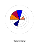
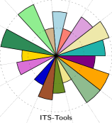
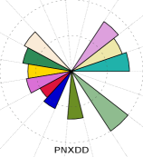
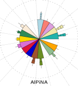
5.3 Radars by models
Figure 1 represents graphically through a set of radar diagrams the highest parameter reached by the tools, for each model. Each diagram corresponds to one model, e.g., echo or Kanban. Each diagram is divided in ten slices, one for each competing tool, always at the same position.
The length of the slice corresponds to the highest parameter reached by the tool. When a slice does not appear, the tool could not process even the smallest parameter. For instance, AlPiNA handles some parameters for eratosthenes and FMS, but is not able to handle the smallest parameter for MAPK. The figure also shows that Marcie handles all parameters for eratosthenes and FMS, but does not reach the highest one for lamport_fmea.
Note that the scale depends on the model : when the parameters of a model vary within a small range (less than ), a linear scale is used (showed using loosely dashed circles as in the Peterson model), whereas a logarithmic scale is used for larger parameter values (showed using densely dashed circles as in the Philosophers model). We also show dotted circles for the results of the tools, in order to allow easier comparison.
Some models (rwmutex and echo) have complex parameters, built from two values. Tools were only able to handle variation of the second parameter, so we only represent it in the figure, in order to show an integer value.

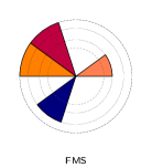


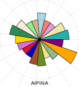
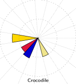
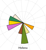
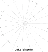
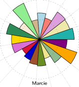
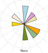
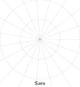
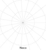
5.4 Radars by tools
Figure 2 presents also radar diagrams showing graphically the participation and results by tool. Each slice in the radars represents a model, always at the same position.
These diagrams differ from those in Figure 1. Each diagram contains two circles: a slice reaches the inner circle if the tool participates to the state space competition for this model, but fails. The size of the slice between the inner and the outer circles represents how many parameters are handled. Its length is the ratio between the number of handled parameters (without failure) and the total number of parameters. Thus, we do not take into account the parameter values.
Two interpretations can rise from the observation of these diagrams:
-
•
First, the colored surface in the inner circle shows how many models could be read by the tool. For instance, AlPiNA, ITS-Tools and Marcie seem to be non-specialized tools, contrary to Crocodile or Neco. This interpretation is biased, as a small surface can also mean that the tool developer did not have time to handle all models.
-
•
Second, the surface between the inner and outer circles shows how well the tool can handle a model. Here, we see that ITS-Tools is very efficient for five models, where it handles all parameters.
Note that LoLa-binstore, LoLa-bloom and Sara did not participate to the state space examination.

5.5 Charts for Models
The charts below correspond to the way tools cope with state space generation for the model that were supported.
Charts for echo
[]
![[Uncaptioned image]](/html/1209.2382/assets/x29.png)
![[Uncaptioned image]](/html/1209.2382/assets/x30.png)
Charts for eratosthenes
[]
![[Uncaptioned image]](/html/1209.2382/assets/x31.png)
![[Uncaptioned image]](/html/1209.2382/assets/x32.png)
Charts for FMS
[]
![[Uncaptioned image]](/html/1209.2382/assets/x33.png)
![[Uncaptioned image]](/html/1209.2382/assets/x34.png)
Charts for galloc_res
[]
![[Uncaptioned image]](/html/1209.2382/assets/x35.png)
![[Uncaptioned image]](/html/1209.2382/assets/x36.png)
Charts for Kanban
[]
![[Uncaptioned image]](/html/1209.2382/assets/x37.png)
![[Uncaptioned image]](/html/1209.2382/assets/x38.png)
Charts for lamport_fmea
[]
![[Uncaptioned image]](/html/1209.2382/assets/x39.png)
![[Uncaptioned image]](/html/1209.2382/assets/x40.png)
Charts for MAPK
[]
![[Uncaptioned image]](/html/1209.2382/assets/x41.png)
![[Uncaptioned image]](/html/1209.2382/assets/x42.png)
Charts for Peterson
[]
![[Uncaptioned image]](/html/1209.2382/assets/x43.png)
![[Uncaptioned image]](/html/1209.2382/assets/x44.png)
Charts for philo_dyn
[]
![[Uncaptioned image]](/html/1209.2382/assets/x45.png)
![[Uncaptioned image]](/html/1209.2382/assets/x46.png)
Charts for Philosophers
[]
![[Uncaptioned image]](/html/1209.2382/assets/x47.png)
![[Uncaptioned image]](/html/1209.2382/assets/x48.png)
Charts for railroad
[]
![[Uncaptioned image]](/html/1209.2382/assets/x49.png)
![[Uncaptioned image]](/html/1209.2382/assets/x50.png)
Charts for ring
[]
![[Uncaptioned image]](/html/1209.2382/assets/x51.png)
![[Uncaptioned image]](/html/1209.2382/assets/x52.png)
Charts for rwmutex
[]
![[Uncaptioned image]](/html/1209.2382/assets/x53.png)
![[Uncaptioned image]](/html/1209.2382/assets/x54.png)
Charts for SharedMemory
[]
![[Uncaptioned image]](/html/1209.2382/assets/x55.png)
![[Uncaptioned image]](/html/1209.2382/assets/x56.png)
Charts for simple_lbs
[]
![[Uncaptioned image]](/html/1209.2382/assets/x57.png)
![[Uncaptioned image]](/html/1209.2382/assets/x58.png)
Charts for TokenRing
[]
![[Uncaptioned image]](/html/1209.2382/assets/x59.png)
![[Uncaptioned image]](/html/1209.2382/assets/x60.png)
5.6 Execution Charts for AlPiNA
We provide here the execution charts observed for AlPiNA over the models it could compete with.
5.6.1 Executions for cs_repetitions
1 chart has been generated.
![[Uncaptioned image]](/html/1209.2382/assets/x61.png)
5.6.2 Executions for echo
1 chart has been generated.
![[Uncaptioned image]](/html/1209.2382/assets/x62.png)
5.6.3 Executions for eratosthenes
7 charts have been generated.
![[Uncaptioned image]](/html/1209.2382/assets/x63.png)
![[Uncaptioned image]](/html/1209.2382/assets/x64.png)
![[Uncaptioned image]](/html/1209.2382/assets/x65.png)
![[Uncaptioned image]](/html/1209.2382/assets/x66.png)
![[Uncaptioned image]](/html/1209.2382/assets/x67.png)
![[Uncaptioned image]](/html/1209.2382/assets/x68.png)
![[Uncaptioned image]](/html/1209.2382/assets/x69.png)
5.6.4 Executions for FMS
5 charts have been generated.
![[Uncaptioned image]](/html/1209.2382/assets/x70.png)
![[Uncaptioned image]](/html/1209.2382/assets/x71.png)
![[Uncaptioned image]](/html/1209.2382/assets/x72.png)
![[Uncaptioned image]](/html/1209.2382/assets/x73.png)
![[Uncaptioned image]](/html/1209.2382/assets/x74.png)
5.6.5 Executions for galloc_res
1 chart has been generated.
![[Uncaptioned image]](/html/1209.2382/assets/x75.png)
5.6.6 Executions for Kanban
4 charts have been generated.
![[Uncaptioned image]](/html/1209.2382/assets/x76.png)
![[Uncaptioned image]](/html/1209.2382/assets/x77.png)
![[Uncaptioned image]](/html/1209.2382/assets/x78.png)
![[Uncaptioned image]](/html/1209.2382/assets/x79.png)
5.6.7 Executions for lamport_fmea
3 charts have been generated.
![[Uncaptioned image]](/html/1209.2382/assets/x80.png)
![[Uncaptioned image]](/html/1209.2382/assets/x81.png)
![[Uncaptioned image]](/html/1209.2382/assets/x82.png)
5.6.8 Executions for MAPK
1 chart has been generated.
![[Uncaptioned image]](/html/1209.2382/assets/x83.png)
5.6.9 Executions for neo-election
1 chart has been generated.
![[Uncaptioned image]](/html/1209.2382/assets/x84.png)
5.6.10 Executions for Peterson
3 charts have been generated.
![[Uncaptioned image]](/html/1209.2382/assets/x85.png)
![[Uncaptioned image]](/html/1209.2382/assets/x86.png)
![[Uncaptioned image]](/html/1209.2382/assets/x87.png)
5.6.11 Executions for philo_dyn
2 charts have been generated.
![[Uncaptioned image]](/html/1209.2382/assets/x88.png)
![[Uncaptioned image]](/html/1209.2382/assets/x89.png)
![[Uncaptioned image]](/html/1209.2382/assets/x90.png)
5.6.12 Executions for Philosophers
8 charts have been generated.
![[Uncaptioned image]](/html/1209.2382/assets/x91.png)
![[Uncaptioned image]](/html/1209.2382/assets/x92.png)
![[Uncaptioned image]](/html/1209.2382/assets/x93.png)
![[Uncaptioned image]](/html/1209.2382/assets/x94.png)
![[Uncaptioned image]](/html/1209.2382/assets/x95.png)
![[Uncaptioned image]](/html/1209.2382/assets/x96.png)
![[Uncaptioned image]](/html/1209.2382/assets/x97.png)
![[Uncaptioned image]](/html/1209.2382/assets/x98.png)
5.6.13 Executions for planning
1 chart has been generated.
![[Uncaptioned image]](/html/1209.2382/assets/x99.png)
5.6.14 Executions for railroad
2 charts have been generated.
![[Uncaptioned image]](/html/1209.2382/assets/x100.png)
![[Uncaptioned image]](/html/1209.2382/assets/x101.png)
5.6.15 Executions for ring
1 chart has been generated.
![[Uncaptioned image]](/html/1209.2382/assets/x102.png)
5.6.16 Executions for rw_mutex
5 charts have been generated.
![[Uncaptioned image]](/html/1209.2382/assets/x103.png)
![[Uncaptioned image]](/html/1209.2382/assets/x104.png)
![[Uncaptioned image]](/html/1209.2382/assets/x105.png)
![[Uncaptioned image]](/html/1209.2382/assets/x106.png)
![[Uncaptioned image]](/html/1209.2382/assets/x107.png)
5.6.17 Executions for simple_lbs
2 charts have been generated.
![[Uncaptioned image]](/html/1209.2382/assets/x108.png)
![[Uncaptioned image]](/html/1209.2382/assets/x109.png)
5.6.18 Executions for SharedMemory
4 charts have been generated.
![[Uncaptioned image]](/html/1209.2382/assets/x110.png)
![[Uncaptioned image]](/html/1209.2382/assets/x111.png)
![[Uncaptioned image]](/html/1209.2382/assets/x112.png)
![[Uncaptioned image]](/html/1209.2382/assets/x113.png)
5.6.19 Executions for ToKenRing
2 charts have been generated.
![[Uncaptioned image]](/html/1209.2382/assets/x114.png)
![[Uncaptioned image]](/html/1209.2382/assets/x115.png)
5.7 Execution Charts for Crocodile
We provide here the execution charts observed for Crocodile over the models it could compete with.
5.7.1 Executions for cs_repetitions
1 chart has been generated.
![[Uncaptioned image]](/html/1209.2382/assets/x116.png)
5.7.2 Executions for galloc_res
2 charts have been generated.
![[Uncaptioned image]](/html/1209.2382/assets/x117.png)
![[Uncaptioned image]](/html/1209.2382/assets/x118.png)
5.7.3 Executions for SharedMemory
6 charts have been generated.
![[Uncaptioned image]](/html/1209.2382/assets/x119.png)
![[Uncaptioned image]](/html/1209.2382/assets/x120.png)
![[Uncaptioned image]](/html/1209.2382/assets/x121.png)
![[Uncaptioned image]](/html/1209.2382/assets/x122.png)
![[Uncaptioned image]](/html/1209.2382/assets/x123.png)
![[Uncaptioned image]](/html/1209.2382/assets/x124.png)
5.8 Execution Charts for Helena
We provide here the execution charts observed for Helena over the models it could compete with.
5.8.1 Executions for lamport_fmea
1 chart has been generated.
![[Uncaptioned image]](/html/1209.2382/assets/x125.png)
5.8.2 Executions for neo-election
1 chart has been generated.
![[Uncaptioned image]](/html/1209.2382/assets/x126.png)
5.8.3 Executions for philo_dyn
6 charts have been generated.
![[Uncaptioned image]](/html/1209.2382/assets/x127.png)
![[Uncaptioned image]](/html/1209.2382/assets/x128.png)
![[Uncaptioned image]](/html/1209.2382/assets/x129.png)
![[Uncaptioned image]](/html/1209.2382/assets/x130.png)
![[Uncaptioned image]](/html/1209.2382/assets/x131.png)
![[Uncaptioned image]](/html/1209.2382/assets/x132.png)
5.8.4 Executions for Philosophers
4 charts have been generated.
![[Uncaptioned image]](/html/1209.2382/assets/x133.png)
![[Uncaptioned image]](/html/1209.2382/assets/x134.png)
![[Uncaptioned image]](/html/1209.2382/assets/x135.png)
![[Uncaptioned image]](/html/1209.2382/assets/x136.png)
5.8.5 Executions for SharedMemory
4 charts have been generated.
![[Uncaptioned image]](/html/1209.2382/assets/x137.png)
![[Uncaptioned image]](/html/1209.2382/assets/x138.png)
![[Uncaptioned image]](/html/1209.2382/assets/x139.png)
![[Uncaptioned image]](/html/1209.2382/assets/x140.png)
5.8.6 Executions for TokenRing
4 charts have been generated.
![[Uncaptioned image]](/html/1209.2382/assets/x141.png)
![[Uncaptioned image]](/html/1209.2382/assets/x142.png)
![[Uncaptioned image]](/html/1209.2382/assets/x143.png)
![[Uncaptioned image]](/html/1209.2382/assets/x144.png)
5.9 Execution Charts for ITS-Tools
We provide here the execution charts observed for ITS-Tools over the models it could compete with.
5.9.1 Executions for echo
1 chart has been generated.
![[Uncaptioned image]](/html/1209.2382/assets/x145.png)
5.9.2 Executions for eratosthenes
7 charts have been generated.
![[Uncaptioned image]](/html/1209.2382/assets/x146.png)
![[Uncaptioned image]](/html/1209.2382/assets/x147.png)
![[Uncaptioned image]](/html/1209.2382/assets/x148.png)
![[Uncaptioned image]](/html/1209.2382/assets/x149.png)
![[Uncaptioned image]](/html/1209.2382/assets/x150.png)
![[Uncaptioned image]](/html/1209.2382/assets/x151.png)
![[Uncaptioned image]](/html/1209.2382/assets/x152.png)
5.9.3 Executions for FMS
7 charts have been generated.
![[Uncaptioned image]](/html/1209.2382/assets/x153.png)
![[Uncaptioned image]](/html/1209.2382/assets/x154.png)
![[Uncaptioned image]](/html/1209.2382/assets/x155.png)
![[Uncaptioned image]](/html/1209.2382/assets/x156.png)
![[Uncaptioned image]](/html/1209.2382/assets/x157.png)
![[Uncaptioned image]](/html/1209.2382/assets/x158.png)
![[Uncaptioned image]](/html/1209.2382/assets/x159.png)
5.9.4 Executions for galloc_res
2 charts have been generated.
![[Uncaptioned image]](/html/1209.2382/assets/x160.png)
![[Uncaptioned image]](/html/1209.2382/assets/x161.png)
5.9.5 Executions for Kanban
8 charts have been generated.
![[Uncaptioned image]](/html/1209.2382/assets/x162.png)
![[Uncaptioned image]](/html/1209.2382/assets/x163.png)
![[Uncaptioned image]](/html/1209.2382/assets/x164.png)
![[Uncaptioned image]](/html/1209.2382/assets/x165.png)
![[Uncaptioned image]](/html/1209.2382/assets/x166.png)
![[Uncaptioned image]](/html/1209.2382/assets/x167.png)
![[Uncaptioned image]](/html/1209.2382/assets/x168.png)
![[Uncaptioned image]](/html/1209.2382/assets/x169.png)
5.9.6 Executions for lamport_fmea
5 charts have been generated.
![[Uncaptioned image]](/html/1209.2382/assets/x171.png)
![[Uncaptioned image]](/html/1209.2382/assets/x172.png)
![[Uncaptioned image]](/html/1209.2382/assets/x173.png)
![[Uncaptioned image]](/html/1209.2382/assets/x174.png)
5.9.7 Executions for MAPK
5 charts have been generated.
![[Uncaptioned image]](/html/1209.2382/assets/x175.png)
![[Uncaptioned image]](/html/1209.2382/assets/x176.png)
![[Uncaptioned image]](/html/1209.2382/assets/x177.png)
![[Uncaptioned image]](/html/1209.2382/assets/x178.png)
![[Uncaptioned image]](/html/1209.2382/assets/x179.png)
5.9.8 Executions for neo-election
1 chart has been generated.
![[Uncaptioned image]](/html/1209.2382/assets/x180.png)
5.9.9 Executions for philo_dyn
6 charts have been generated.
![[Uncaptioned image]](/html/1209.2382/assets/x181.png)
![[Uncaptioned image]](/html/1209.2382/assets/x182.png)
![[Uncaptioned image]](/html/1209.2382/assets/x183.png)
5.9.10 Executions for Philosophers
13 charts have been generated.
![[Uncaptioned image]](/html/1209.2382/assets/x184.png)
![[Uncaptioned image]](/html/1209.2382/assets/x185.png)
![[Uncaptioned image]](/html/1209.2382/assets/x186.png)
![[Uncaptioned image]](/html/1209.2382/assets/x187.png)
![[Uncaptioned image]](/html/1209.2382/assets/x188.png)
![[Uncaptioned image]](/html/1209.2382/assets/x189.png)
![[Uncaptioned image]](/html/1209.2382/assets/x190.png)
![[Uncaptioned image]](/html/1209.2382/assets/x191.png)
![[Uncaptioned image]](/html/1209.2382/assets/x192.png)
![[Uncaptioned image]](/html/1209.2382/assets/x193.png)
![[Uncaptioned image]](/html/1209.2382/assets/x194.png)
![[Uncaptioned image]](/html/1209.2382/assets/x195.png)
![[Uncaptioned image]](/html/1209.2382/assets/x196.png)
5.9.11 Executions for planning
1 chart has been generated.
![[Uncaptioned image]](/html/1209.2382/assets/x197.png)
5.9.12 Executions for railroad
3 charts have been generated.
![[Uncaptioned image]](/html/1209.2382/assets/x198.png)
![[Uncaptioned image]](/html/1209.2382/assets/x199.png)
![[Uncaptioned image]](/html/1209.2382/assets/x200.png)
5.9.13 Executions for ring
1 chart has been generated.
![[Uncaptioned image]](/html/1209.2382/assets/x201.png)
5.9.14 Executions for rw_mutex
4 charts have been generated.
![[Uncaptioned image]](/html/1209.2382/assets/x202.png)
![[Uncaptioned image]](/html/1209.2382/assets/x203.png)
![[Uncaptioned image]](/html/1209.2382/assets/x204.png)
![[Uncaptioned image]](/html/1209.2382/assets/x205.png)
![[Uncaptioned image]](/html/1209.2382/assets/x206.png)
5.9.15 Executions for SharedMemory
4 charts have been generated.
![[Uncaptioned image]](/html/1209.2382/assets/x207.png)
![[Uncaptioned image]](/html/1209.2382/assets/x208.png)
![[Uncaptioned image]](/html/1209.2382/assets/x209.png)
![[Uncaptioned image]](/html/1209.2382/assets/x210.png)
5.9.16 Executions for simple_lbs
5 charts have been generated.
![[Uncaptioned image]](/html/1209.2382/assets/x211.png)
![[Uncaptioned image]](/html/1209.2382/assets/x212.png)
![[Uncaptioned image]](/html/1209.2382/assets/x213.png)
![[Uncaptioned image]](/html/1209.2382/assets/x214.png)
![[Uncaptioned image]](/html/1209.2382/assets/x215.png)
5.9.17 Executions for TokenRing
4 charts have been generated.
![[Uncaptioned image]](/html/1209.2382/assets/x216.png)
![[Uncaptioned image]](/html/1209.2382/assets/x217.png)
![[Uncaptioned image]](/html/1209.2382/assets/x218.png)
![[Uncaptioned image]](/html/1209.2382/assets/x219.png)
5.10 Execution Charts for Marcie
We provide here the execution charts observed for Marcie over the models it could compete with.
5.10.1 Executions for cs_repetitions
1 chart has been generated.
![[Uncaptioned image]](/html/1209.2382/assets/x220.png)
5.10.2 Executions for echo
2 charts have been generated.
![[Uncaptioned image]](/html/1209.2382/assets/x221.png)
![[Uncaptioned image]](/html/1209.2382/assets/x222.png)
5.10.3 Executions for eratosthenes
7 charts have been generated.
![[Uncaptioned image]](/html/1209.2382/assets/x223.png)
![[Uncaptioned image]](/html/1209.2382/assets/x224.png)
![[Uncaptioned image]](/html/1209.2382/assets/x225.png)
![[Uncaptioned image]](/html/1209.2382/assets/x226.png)
![[Uncaptioned image]](/html/1209.2382/assets/x227.png)
![[Uncaptioned image]](/html/1209.2382/assets/x228.png)
![[Uncaptioned image]](/html/1209.2382/assets/x229.png)
5.10.4 Executions for FMS
7 charts have been generated.
![[Uncaptioned image]](/html/1209.2382/assets/x230.png)
![[Uncaptioned image]](/html/1209.2382/assets/x231.png)
![[Uncaptioned image]](/html/1209.2382/assets/x232.png)
![[Uncaptioned image]](/html/1209.2382/assets/x233.png)
![[Uncaptioned image]](/html/1209.2382/assets/x234.png)
![[Uncaptioned image]](/html/1209.2382/assets/x235.png)
![[Uncaptioned image]](/html/1209.2382/assets/x236.png)
5.10.5 Executions for galloc_res
2 charts have been generated.
![[Uncaptioned image]](/html/1209.2382/assets/x237.png)
![[Uncaptioned image]](/html/1209.2382/assets/x238.png)
5.10.6 Executions for Kanban
6 charts have been generated.
![[Uncaptioned image]](/html/1209.2382/assets/x239.png)
![[Uncaptioned image]](/html/1209.2382/assets/x240.png)
![[Uncaptioned image]](/html/1209.2382/assets/x241.png)
![[Uncaptioned image]](/html/1209.2382/assets/x242.png)
![[Uncaptioned image]](/html/1209.2382/assets/x243.png)
![[Uncaptioned image]](/html/1209.2382/assets/x244.png)
5.10.7 Executions for lamport_fmea
3 charts have been generated.
![[Uncaptioned image]](/html/1209.2382/assets/x245.png)
![[Uncaptioned image]](/html/1209.2382/assets/x246.png)
![[Uncaptioned image]](/html/1209.2382/assets/x247.png)
5.10.8 Executions for neo-election
1 chart has been generated.
![[Uncaptioned image]](/html/1209.2382/assets/x248.png)
5.10.9 Executions for Peterson
2 charts have been generated.
![[Uncaptioned image]](/html/1209.2382/assets/x249.png)
![[Uncaptioned image]](/html/1209.2382/assets/x250.png)
5.10.10 Executions for philo_dyn
3 charts have been generated.
![[Uncaptioned image]](/html/1209.2382/assets/x251.png)
![[Uncaptioned image]](/html/1209.2382/assets/x252.png)
![[Uncaptioned image]](/html/1209.2382/assets/x253.png)
5.10.11 Executions for Philosophers
10 charts have been generated.
![[Uncaptioned image]](/html/1209.2382/assets/x254.png)
![[Uncaptioned image]](/html/1209.2382/assets/x255.png)
![[Uncaptioned image]](/html/1209.2382/assets/x256.png)
![[Uncaptioned image]](/html/1209.2382/assets/x257.png)
![[Uncaptioned image]](/html/1209.2382/assets/x258.png)
![[Uncaptioned image]](/html/1209.2382/assets/x259.png)
![[Uncaptioned image]](/html/1209.2382/assets/x260.png)
![[Uncaptioned image]](/html/1209.2382/assets/x261.png)
![[Uncaptioned image]](/html/1209.2382/assets/x262.png)
![[Uncaptioned image]](/html/1209.2382/assets/x263.png)
5.10.12 Executions for railroad
3 charts have been generated.
![[Uncaptioned image]](/html/1209.2382/assets/x264.png)
![[Uncaptioned image]](/html/1209.2382/assets/x265.png)
![[Uncaptioned image]](/html/1209.2382/assets/x266.png)
5.10.13 Executions for ring
1 chart has been generated.
![[Uncaptioned image]](/html/1209.2382/assets/x267.png)
5.10.14 Executions for rw_mutex
5 charts have been generated.
![[Uncaptioned image]](/html/1209.2382/assets/x268.png)
![[Uncaptioned image]](/html/1209.2382/assets/x269.png)
![[Uncaptioned image]](/html/1209.2382/assets/x270.png)
![[Uncaptioned image]](/html/1209.2382/assets/x271.png)
![[Uncaptioned image]](/html/1209.2382/assets/x272.png)
5.10.15 Executions for SharedMemory
7 charts have been generated.
![[Uncaptioned image]](/html/1209.2382/assets/x273.png)
![[Uncaptioned image]](/html/1209.2382/assets/x274.png)
![[Uncaptioned image]](/html/1209.2382/assets/x275.png)
![[Uncaptioned image]](/html/1209.2382/assets/x276.png)
![[Uncaptioned image]](/html/1209.2382/assets/x277.png)
![[Uncaptioned image]](/html/1209.2382/assets/x278.png)
![[Uncaptioned image]](/html/1209.2382/assets/x279.png)
5.10.16 Executions for simple_lbs
3 charts have been generated.
![[Uncaptioned image]](/html/1209.2382/assets/x280.png)
![[Uncaptioned image]](/html/1209.2382/assets/x281.png)
![[Uncaptioned image]](/html/1209.2382/assets/x282.png)
5.10.17 Executions for TokenRing
4 charts have been generated.
![[Uncaptioned image]](/html/1209.2382/assets/x283.png)
![[Uncaptioned image]](/html/1209.2382/assets/x284.png)
![[Uncaptioned image]](/html/1209.2382/assets/x285.png)
![[Uncaptioned image]](/html/1209.2382/assets/x286.png)
5.11 Execution Charts for Neco
We provide here the execution charts observed for Neco over the models it could compete with.
5.11.1 Executions for eratosthenes
4 charts have been generated.
![[Uncaptioned image]](/html/1209.2382/assets/x287.png)
![[Uncaptioned image]](/html/1209.2382/assets/x288.png)
![[Uncaptioned image]](/html/1209.2382/assets/x289.png)
![[Uncaptioned image]](/html/1209.2382/assets/x290.png)
5.11.2 Executions for Kanban
2 charts have been generated.
![[Uncaptioned image]](/html/1209.2382/assets/x291.png)
![[Uncaptioned image]](/html/1209.2382/assets/x292.png)
5.11.3 Executions for MAPK
2 charts have been generated.
![[Uncaptioned image]](/html/1209.2382/assets/x293.png)
![[Uncaptioned image]](/html/1209.2382/assets/x294.png)
5.11.4 Executions for Peterson
2 charts have been generated.
![[Uncaptioned image]](/html/1209.2382/assets/x295.png)
![[Uncaptioned image]](/html/1209.2382/assets/x296.png)
5.11.5 Executions for philo_dyn
3 charts have been generated.
![[Uncaptioned image]](/html/1209.2382/assets/x297.png)
![[Uncaptioned image]](/html/1209.2382/assets/x298.png)
![[Uncaptioned image]](/html/1209.2382/assets/x299.png)
5.11.6 Executions for rw_mutex
5 charts have been generated.
![[Uncaptioned image]](/html/1209.2382/assets/x300.png)
![[Uncaptioned image]](/html/1209.2382/assets/x301.png)
![[Uncaptioned image]](/html/1209.2382/assets/x302.png)
![[Uncaptioned image]](/html/1209.2382/assets/x303.png)
![[Uncaptioned image]](/html/1209.2382/assets/x304.png)
5.11.7 Executions for simple_lbs
3 charts have been generated.
![[Uncaptioned image]](/html/1209.2382/assets/x305.png)
![[Uncaptioned image]](/html/1209.2382/assets/x306.png)
![[Uncaptioned image]](/html/1209.2382/assets/x307.png)
5.12 Execution Charts for PNXDD
We provide here the execution charts observed for PNXDD over the models it could compete with.
5.12.1 Executions for cs_repetitions
1 chart has been generated.
![[Uncaptioned image]](/html/1209.2382/assets/x308.png)
5.12.2 Executions for FMS
6 charts have been generated.
![[Uncaptioned image]](/html/1209.2382/assets/x309.png)
![[Uncaptioned image]](/html/1209.2382/assets/x310.png)
![[Uncaptioned image]](/html/1209.2382/assets/x311.png)
![[Uncaptioned image]](/html/1209.2382/assets/x312.png)
![[Uncaptioned image]](/html/1209.2382/assets/x313.png)
![[Uncaptioned image]](/html/1209.2382/assets/x314.png)
5.12.3 Executions for galloc_res
2 charts have been generated.
![[Uncaptioned image]](/html/1209.2382/assets/x315.png)
![[Uncaptioned image]](/html/1209.2382/assets/x316.png)
5.12.4 Executions for Kanban
5 charts have been generated.
![[Uncaptioned image]](/html/1209.2382/assets/x317.png)
![[Uncaptioned image]](/html/1209.2382/assets/x318.png)
![[Uncaptioned image]](/html/1209.2382/assets/x319.png)
![[Uncaptioned image]](/html/1209.2382/assets/x320.png)
![[Uncaptioned image]](/html/1209.2382/assets/x321.png)
5.12.5 Executions for MAPK
5 charts have been generated.
![[Uncaptioned image]](/html/1209.2382/assets/x322.png)
![[Uncaptioned image]](/html/1209.2382/assets/x323.png)
![[Uncaptioned image]](/html/1209.2382/assets/x324.png)
![[Uncaptioned image]](/html/1209.2382/assets/x325.png)
![[Uncaptioned image]](/html/1209.2382/assets/x326.png)
5.12.6 Executions for Peterson
4 charts have been generated.
![[Uncaptioned image]](/html/1209.2382/assets/x327.png)
![[Uncaptioned image]](/html/1209.2382/assets/x328.png)
![[Uncaptioned image]](/html/1209.2382/assets/x329.png)
![[Uncaptioned image]](/html/1209.2382/assets/x330.png)
5.12.7 Executions for philo_dyn
3 charts have been generated.
![[Uncaptioned image]](/html/1209.2382/assets/x331.png)
![[Uncaptioned image]](/html/1209.2382/assets/x332.png)
![[Uncaptioned image]](/html/1209.2382/assets/x333.png)
5.12.8 Executions for Philosophers
6 charts have been generated.
![[Uncaptioned image]](/html/1209.2382/assets/x334.png)
![[Uncaptioned image]](/html/1209.2382/assets/x335.png)
![[Uncaptioned image]](/html/1209.2382/assets/x336.png)
![[Uncaptioned image]](/html/1209.2382/assets/x337.png)
![[Uncaptioned image]](/html/1209.2382/assets/x338.png)
![[Uncaptioned image]](/html/1209.2382/assets/x339.png)
5.12.9 Executions for SharedMemory
4 charts have been generated.
![[Uncaptioned image]](/html/1209.2382/assets/x340.png)
![[Uncaptioned image]](/html/1209.2382/assets/x341.png)
![[Uncaptioned image]](/html/1209.2382/assets/x342.png)
![[Uncaptioned image]](/html/1209.2382/assets/x343.png)
5.12.10 Executions for simple_lbs
5 charts have been generated.
![[Uncaptioned image]](/html/1209.2382/assets/x344.png)
![[Uncaptioned image]](/html/1209.2382/assets/x345.png)
![[Uncaptioned image]](/html/1209.2382/assets/x346.png)
![[Uncaptioned image]](/html/1209.2382/assets/x347.png)
![[Uncaptioned image]](/html/1209.2382/assets/x348.png)
5.12.11 Executions for TokenRing
3 charts have been generated.
![[Uncaptioned image]](/html/1209.2382/assets/x349.png)
![[Uncaptioned image]](/html/1209.2382/assets/x350.png)
![[Uncaptioned image]](/html/1209.2382/assets/x351.png)
6 Raw Data for Structural Formulæ Evaluation
This section shows the raw results of the structural formulæ examination. Table 4 summarizes the highest scaling parameter reached by the tools for each model. Then Charts generated from the data collected for this examination are provided. This table should be interpreted using the legend displayed in Section 5, page 5. Let us not that only two tools did participate in the evaluation of structural formulæ: AlPiNA and Helena. LoLa-binstore, LoLa-bloom and Sara could not compete because of the combination of structural assertions.
| AlPiNA | Crocodile | Helena | ITS-Tools | LoLA (binstore) | LoLA (bloom) | Marcie | Neco | PNXDD | Sara | ||
|---|---|---|---|---|---|---|---|---|---|---|---|
| MCC 2011 models | FMS | 10 P | |||||||||
| Kanban | 20 P | ||||||||||
| MAPK | |||||||||||
| Peterson | 2 C | ||||||||||
| Philosophers | 10 C | ||||||||||
| Shared-Memory | 10 C | 20 C | |||||||||
| TokenRing | 20 C | ||||||||||
| new models from MCC 2012 | Cs_repetitions | ||||||||||
| Echo | |||||||||||
| Eratosthenes | |||||||||||
| Galloc_res | |||||||||||
| Lamport_fmea | 3 C | 5 C | |||||||||
| NEO-election | |||||||||||
| Philo_dyn | 3 C | 20 C | |||||||||
| Planning | |||||||||||
| Railroad | |||||||||||
| Ring | |||||||||||
| Rw_mutex | r10w100 P | ||||||||||
| Simple_lbs | 2 P | 15 C | |||||||||
Section 6.1 presents the data computed by tools. Then, Section 6.2 shows how models have been handled by tools and Sections 6.4 and 6.3 summarize how tools did cope with models.
Section 6.1 shows that no tool computes the same set of formulæ. This is why we do not display the charts that have been extracted from the executions since they have no meaning at all.
6.1 Computed results for the formulæ
Since only two tools did compete and had sometimes different results, we could not consolidate the values and decided to show the results as they were produced in Table 5. For each scaling parameter, we proposed a set of formulæ. Outputs from the tools were analyzed and formula were sorted by their identifier in order to build a vector where the element corresponds to the formula of the set (value F or T). Sometimes, the tool cannot compute a formula. We then display a “.” instead. For this examination, it appears that, the problem is often due to formula evaluation itself (the grammar was published late and thus). "?" means that the tool participated but did not compute any result.
| Scale | AlPiNA | Helena |
| value | ||
| cs_repetitions | ||
| 25 | ? | |
| echo | ||
| d2r11 | ? | |
| eratosthenes | ||
| 5 | ? | |
| FMS | ||
| 2 | …………………..FFFFFTTTT.FTTTTTTTTT.TFFFFF….. | |
| 5 | …………………..FFFFFFFFF.FFFFFFFFFF.FTTTTFFTFT.T…. | |
| 10 | …………………..FFFFFFFFF.FFTFTFFTFT.TFTFFFFTFT.TFTFTFFFFF.F… | |
| galloc_res | ||
| 3 | ? | |
| Kanban | ||
| 5 | …………………..FFFFFFFFF.FFFFFFFFFF.FTTTTFFFFF.F…. | |
| 10 | …………………..FFFFFFFFF.FFFFFFFFFF.FFFFFFFFFF.FFFFFFFFFF.F… | |
| 20 | …………………..FFFFFFFFF.FFFFFFFFFF.FFFFFFFFFF.FFFFFFFFFF.FFFFFFFFFF.F.. | |
| lamport_fmea | ||
| 2 | TTTTTTTTFTFTTTFFTTTFFTTTTTTTTTFTFTTTTTTT | ……….T……………………….. |
| 3 | FTTFFFTTFTFFTTTTFTTFTTTTTTTTTTFTFTTTTTTTTFTTTFFTFT | ………………………………………….. |
| 4 | ? | ………………………………………….. |
| 5 | ? | ………………………………………….. |
| MAPK | ||
| 8 | ? | |
| Peterson | ||
| 2 | TFTFFFTTTTFTTTFTTTTFFFFTTTTFTTTTFTTTFTFFTFTFFFFTFF | |
| philo_dyn | ||
| 2 | FTTTTTTTFFFFTTTTTFTFTFFFFFFFFF | ……….T………………. |
| 3 | FTTTTTTTFFFFTTTTTFTFTFFFFFFFFF | …………………………………. |
| 10 | ? | ………………………………………………. |
| 20 | ? | ………………………………………………. |
| Philosophers | ||
| 5 | FFTFFFFTFFFFFTFFFTTFTFTFFFFFFF | |
| 10 | FFFFFFFFFFFFFFFFFFTFTFFFTFTFFTFTFFFFFFFF | |
| planning | ||
| — | ? | |
| ring | ||
| — | ? | |
| rwmutex | ||
| r10w10 | …………………..FFFFFTTTT.FTTFTFFTFT.F….. | |
| r10w20 | …………………..FFFFTTTFT.TTTTTTTTTT.T….. | |
| r10w50 | …………………..FFFFFTTTT.FTTFTTTTTT.F….. | |
| r10w100 | …………………..FFFFFTTTT.FTTTTTFFFF.F….. | |
| SharedMemory | ||
| 5 | TFTFTFFTFTFTFTFTFTTFTFFTTTTTTTFTFTTTFTFFFFFFFFFTFF | ………………………………………….. |
| 10 | FFTFTFFTFFFFFTFTFFTFFFTTTTTTTTTTFFTTTTTTTFTFFFTFTTFFTFT | ………………………………………………. |
| 20 | ? | ………………………………………………. |
| simple_lbs | ||
| 2 | TTTTTTTTFTFFTTFTFTTFFFFFFFFTFF | ……….T………………. |
| 5 | ? | …………………………………. |
| 10 | ? | ………………………………………….. |
| 15 | ? | ………………………………………….. |
| TokenRing | ||
| 2 | ? | ……….T………………………………… |
| 10 | ? | ………………………………………………. |
| 20 | ? | ………………………………………………. |
6.2 Processed Models
This section summarizes how models were processed by tools. Let us first note that no tool succeeded in this examination for the following models:
-
•
cs_repetitions,
-
•
echo,
-
•
eratosthenes,
-
•
galloc_res,
-
•
MAPK,
-
•
neo-election,
-
•
planning,
-
•
railroad,
-
•
ring.
These models constitute challenges for the next edition of the Model Checking Contest.
6.3 Radars by models
Figure 3 represents graphically through a set of radar diagrams the highest parameter reached by the tools, for each model. Each diagram corresponds to one model, e.g., echo or Kanban. Each diagram is divided in ten slices, one for each competing tool, always at the same position.
The length of the slice corresponds to the highest parameter reached by the tool. When a slice does not appear, the tool could not process even the smallest parameter. For instance, Helena handles some parameters for lamport_fmea and TokenRing, but is not able to handle the smallest parameter for eratosthenes. The figure also shows that only two tools (AlPiNA and Helena) did compete for this examination. None of them achieves the highest parameter for any model.
Note that the scale depends on the model : when the parameters of a model vary within a small range (less than ), a linear scale is used (showed using loosely dashed circles as in the Peterson model), whereas a logarithmic scale is used for larger parameter values (showed using densely dashed circles as in the Philosophers model). We also show dotted circles for the results of the tools, in order to allow easier comparison.
Some models (rwmutex and echo) have complex parameters, built from two values. Tools were only able to handle variation of the second parameter, so we only represent it in the figure, in order to show an integer value.


6.4 Radars by tools
Figure 4 presents also radar diagrams showing graphically the participation and results by tool. Each slice in the radars represents a model, always at the same position.
These diagrams differ from both those in Figure 3 and those in Figure 1. Each diagram contains two circles, as in Figure 1: a slice reaches the inner circle if the tool participates to the state space competition for this model, but fails. The number of subslices between the inner and the outer circles represents how many parameters are handled. The angle covered by each subslice shows the ratio between the computed formulæ and the total number of formulæ in the examination. For instance, AlPiNA has wider subslices than Helena: it is able to handle more formulæ. But its subslices do not cover the whole angle dedicated to each model: AlPiNA could not handle all the formulæ proposed in this examination.
The colored surface in the inner circle shows if the tool could at least handle one formula for the model. For instance, AlPiNA and Helena could handle formulæ for simple_lbs, but not for railroad.
This figure is not sufficient as we do not clearly distinguish tools that try to handle formulæ from tools that do not compete. For instance, AlPiNA tries for all models, but has four “blank” models in the figure.


7 Raw Data for Reachability Formulæ Evaluation
This section shows the raw results of the reachability formulæ examination. Table 6 summarizes the highest scaling parameter reached by the tools for each model. Then Charts generated from the data collected for this examination are provided. This table should be interpreted using the legend displayed in page 5.
| AlPiNA | Crocodile | Helena | ITS-Tools | LoLA (binstore) | LoLA (bloom) | Marcie | Neco | PNXDD | Sara | ||
|---|---|---|---|---|---|---|---|---|---|---|---|
| MCC 2011 models | FMS | 10 P | 500 P | 500 P | |||||||
| Kanban | 20 P | 1 000 P | 1 000 P | ||||||||
| MAPK | 320 P | 320 P | |||||||||
| Peterson | 2 C | 4 P | 5 P | ||||||||
| Philosophers | 10 C | 50 000 P | |||||||||
| Shared-Memory | 5 C | 20 C | |||||||||
| TokenRing | 20 C | ||||||||||
| new models from MCC 2012 | Cs_repetitions | 225 P | 900 P | ||||||||
| Echo | d2r11 P | d2r11 P | d2r11 P | ||||||||
| Eratosthenes | 500 P | 500 P | |||||||||
| Galloc_res | 3 P | 5 P | |||||||||
| Lamport_fmea | 3 C | 5 C | 4 P | ||||||||
| NEO-election | 8 P | ||||||||||
| Philo_dyn | 3 C | 20 C | 20 P | ||||||||
| Planning | |||||||||||
| Railroad | |||||||||||
| Ring | |||||||||||
| Rw_mutex | r10w100 P | r2000w10 P | r2000w10 P | r20w10 P | |||||||
| Simple_lbs | 2 P | 15 C | 5 P | 20 P | 20 P | ||||||
Section 7.1 presents the data computed by tools. Then, Section 7.2 shows how models have been handled by tools and Section 7.3 summarizes how tools did cope with models.
Section 7.1 shows that no tool compute the same set of formulæ. This is why we do not display the charts that have been extracted from the executions since they have no meaning at all.
7.1 Computed results for the formulæ
Since the participating tools did produce various values, we could not consolidate the results and decided to show them as they were produced in Tables 7 and 8. We use the notations already presented for Table 5, page 5 (use of T, F or “.” in the issued vector).
| Scale | AlPiNA | Helena | LoLa-binstore | LoLa-bloom | Sara |
| cs_repetitions | |||||
| 25 | T……………………… | ….FFFTTT……………… | |||
| 49 | T……………………… | ….TTT………………FFT | |||
| 100 | T……………………… | ….TTT…TTT…………… | |||
| 225 | T……………………… | ….TTT………………… | |||
| 400 | ? | ……….FFF…………… | |||
| 625 | ? | ………….TTT………FFF | |||
| 900 | ? | ….TTT…TTT…………… | |||
| echo | |||||
| s2r11 | ? | T…FFFFFFFFFFFFFFFFFF | ….F.FF.FF..FF.F..FFF | ………….FFF…… | |
| eratosthenes | |||||
| 5 | ? | ………….. | ………….. | .FFFF…FFFF.. | |
| 10 | ? | ………….. | .FFFF…FFFF.. | ||
| 20 | ? | ………….. | .FFFF…FFFF.. | ||
| 50 | ? | ………….. | .FFFF…FFFF.. | ||
| 100 | ? | ………….. | .FFFF…FFFF.. | ||
| 200 | ? | ………….. | .FFFF…FFFF.. | ||
| 500 | ? | ………….. | .FFFF…FFFF.. | ||
| FMS | |||||
| 2 | ….FFFFFFFTFFFFFFFFFF | F…FFFFFFFTFFFFFFFFFF | ….FFFFF.F.FFFFF..F.F | …………….TTT… | |
| 5 | ….FFFFFFFFFFFFFFFFFF | F…FFFFFFFFFFFFFFFFFF | ….F..FFF………..F | …………….TTT… | |
| 10 | ….FFFFFFFFFFFFFFFFFF | F…FFFFFFFFFFFFFFFFFF | ….F..F..F….FFFF… | ||
| 20 | ? | FFFF…FFFFFFFFFFFFFFF | FFF….FFFFFF…FF…F | ||
| 50 | ? | FFFF…FFFFFFFFFFFFFFF | ..F….FF….FF…FF.F | ||
| 100 | ? | FFFFFFFFF…FFFFFFFFFF | F.FFFF.F….F..F.FF..F | ||
| 200 | ? | FFFFFFFFF…FFFFFFFFFF | .F..FF………F….FF | ||
| 500 | ? | FFFFFFFFF…FFFFFFFFFF | ..F..FF…..F..FFFF.FF | ||
| galloc_res | |||||
| 3 | ? | F……………………… | …….FFF…TTF………… | ||
| 5 | ? | ……….TTT…………… | |||
| Kanban | |||||
| 5 | ….FFFFFFFFFFFFFFFFFF | F…FFFFFFFFFFFFFFFFFF | ….F.FFFFF..F..FF.F.. | ….TTT………TTF… | |
| 10 | ….FTFFFFFFFFFFFFFFFF | F…FTFFFFFFFFFFFFFFFF | ….F..FFFF..F.FF.FF.F | ||
| 20 | FFF….FFFFFFFFFFFFFFF | FFFF…FFFFFFFFFFFFFFF | FF…..FFFF.FFFFF..FFF | ||
| 50 | ? | FFFF…FFFFFFFFFFFFFFF | F……..FF….F..FF.F | ||
| 100 | ? | FFFFFFFF….FFFFFFFFFF | ..FFF……….FFFF… | ||
| 200 | ? | FFFFFFFF….FFFFF.FFFF | ….FFF…..F.FFF.F.FF | ||
| 500 | ? | FFFFFFFF….FFFFFFFFFF | .F……….FFFF..FF.F | ||
| 1 000 | ? | FFFFFFFF….FFFFFFFFFF | ..FFFFFF……FF..F… | ||
| lamport_fmea | |||||
| 2 | ………………….FFF… | T……………………… | F……………………… | ||
| 3 | …………………….FFF | T……………………… | F……………………… | ||
| 4 | ? | T……………………… | F……………………… | ||
| 5 | ? | T……………………… | ? | ||
| MAPK | |||||
| 8 | ? | F…FFFFFFFFFFTFFFFFFF | ….FF.F.FF..F.FFFFFF. | ….TTT………FTT… | |
| 20 | ? | FFF….FFFFFFFFFFFFFFF | F………..FFFFF..F.F | ||
| 40 | ? | FFF….FFFFFFFFFFFFFFF | F……F.FFFFF…….. | ||
| 80 | ? | FFFFFFFF….FFFFFFFFFF | F…FF……FF.FF.F..F | ||
| 160 | ? | FFFFFFFF….FFFFFFFFFF | .FFF.FFF…….FF.FFFF | ||
| 320 | ? | FFFFFFFF….FFFFFFFF.F | .FF.F…….F.F..FF..F | ||
| neo-election | |||||
| 2 | T……………………… | ||||
| 3 | T……………………… | ||||
| 4 | T……………………… | ||||
| 5 | T……………………… | ||||
| 6 | T……………………… | ||||
| 7 | T……………………… | ||||
| 8 | T……………………… | ||||
| Scale | AlPiNA | Helena | LoLa-binstore | LoLa-bloom | Sara |
| Peterson | |||||
| 2 | ….FFFFFFFFFFFF……FFFFFF | ? | F……………………… | ……….FFT…………… | |
| 3 | ? | ? | F……………………… | ………………….TTTFFT | |
| 4 | ? | ? | F……………………… | ………………….TTTTTT | |
| 5 | ? | ? | ? | ………………….TTT… | |
| philo_dyn | |||||
| 2 | ….FFFFFFFFFFFF……FFFFFF | T……………………… | T……………………… | ||
| 3 | ….FTTFFFFFFFTF……FFFFFF | F……………………… | T……………………… | ||
| 10 | ? | F……………………… | T……………………… | ||
| 20 | ? | F……………………… | T……………………… | ||
| Philosophers | |||||
| 5 | ….FFFFFFFFFFFF……FFFFFF | T……………………… | ……….TTT…………… | ||
| 10 | ….FFFFFFFFFFFF……FFFFFF | T……………………… | |||
| 20 | ? | T……………………… | |||
| 50 | ? | T……………………… | |||
| 100 | ? | T……………………… | |||
| 200 | ? | T……………………… | |||
| 500 | ? | T……………………… | |||
| 1 000 | ? | T……………………… | |||
| 2 000 | ? | T……………………… | |||
| 5 000 | ? | T……………………… | |||
| 10 000 | ? | T……………………… | |||
| 50 000 | ? | T……………………… | |||
| rwmutex | |||||
| r10w10 | ….FFFFTFFFFFFFFFFFFF | F…FFFFFFFFFFFFFFFFFF | ….F.FFF.F..FFFFFF… | ……….FFT…FTT… | |
| r10w20 | ….FFFFFFFFFFTFFFFFFF | F…FFFFFFFFFFTFFTFFFF | ….FFF…F..F.FF.F… | ……….TTF……TTT | |
| r10w50 | ….FFFFTTFFFFFFFFFFTF | F…FFTFFFFTFFFFFTFFTF | ….FF.FFF..FF.F…F.. | …………….TTT… | |
| r10w100 | ….FTFFFFFFFFFTFFFFFT | F…FFFFFFFFFFTFFFFFTF | ….F..FF.F…..FFF… | ….TTT…………… | |
| r10w500 | ? | F…FTFFFFFFFFFFFFFFTF | …….FF.FF.FF.F.FF.F | ……….TTT……… | |
| r10w1000 | ? | F…FTFFTTFTFFFTFFFFFF | ……FF….FF..F..F.. | ….TTT…TTT……… | |
| r10w2000 | ? | F…FTFFFFFFFFFFFFTFFF | ……FF.FF.FFFFF..FFF | ……….TTT……… | |
| r20w10 | ? | F…FFFFFFFFFFFFFFFFFF | ….F…..FF.FF……F | ….FFT…………… | |
| r100w10 | ? | F…FFFFFFFFFFFFFFFFFF | ….FF.F..FFFF.FF.FFF. | ||
| r500w10 | ? | F…FFFFFFFFFFFFFFFFFF | ……F…F..F.FF..FF. | ||
| r1000w10 | ? | F…FFFFFFFFFFFFFFFFFF | …….F.FF.FFF.FF…F | ||
| r2000w10 | ? | F…FFFFFFFFFFFFFFFFFF | ….F.FF.FFFFF…..FF. | ||
| SharedMemory | |||||
| 5 | ….FFFFFFFTFFFF……FFFFFF | T……………………… | |||
| 10 | ? | T……………………… | |||
| 20 | ? | T……………………… | |||
| simple_lbs | |||||
| 2 | ……….FFFFFF………… | T……………………… | F…FTFFTFFFFFFF……FFFFFF | ….F.F…F.FF.F………F.F | …………….FT………. |
| 5 | ? | T……………………… | F…FFFFFFFFFFFF……FFFFFF | ….F..F..F..F.F……FF.FFF | …………….TTT……… |
| 10 | ? | T……………………… | ? | ….F.FF..F..F.F……FFFF.. | …………….F.F……… |
| 15 | ? | T……………………… | ? | …….F.FF.FFFF……F..FF. | …………….F…..FFT… |
| 20 | ? | ? | ….F..F.FF..F.F……F..FFF | …….TT…….F……….. | |
| TokenRing | |||||
| 5 | T…………… | ||||
| 10 | T…………… | ||||
| 20 | T…………… | ||||
7.2 Processed Models
This section summarizes how models were processed by tools. Let us first note that no tool succeeded in this examination for the following models:
-
•
planning,
-
•
railroad,
-
•
ring.
These models constitute challenges for the next edition of the Model Checking Contest.
7.3 Radars by models
Figure 5 represents graphically through a set of radar diagrams the highest parameter reached by the tools, for each model. Each diagram corresponds to one model, e.g., echo or Kanban. Each diagram is divided in ten slices, one for each competing tool, always at the same position.
The length of the slice corresponds to the highest parameter reached by the tool. When a slice does not appear, the tool could not process even the smallest parameter. For instance, LoLa-binstore handles some parameters for almost all models (and the highest parameter for most of them), but is not able to handle the smallest parameter for SharedMemory.
Note that the scale depends on the model : when the parameters of a model vary within a small range (less than ), a linear scale is used (showed using loosely dashed circles as in the Peterson model), whereas a logarithmic scale is used for larger parameter values (showed using densely dashed circles as in the Philosophers model). We also show dotted circles for the results of the tools, in order to allow easier comparison.
Some models (rwmutex and echo) have complex parameters, built from two values. Tools were only able to handle variation of the second parameter, so we only represent it in the figure, in order to show an integer value.
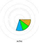
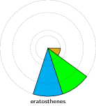
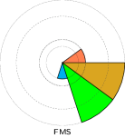
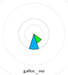
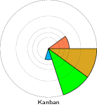
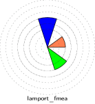
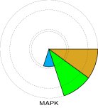

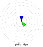


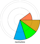
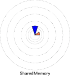
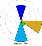
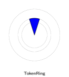

7.4 Radars by tools
Figure 6 presents also radar diagrams showing graphically the participation and results by tool. Each slice in the radars represents a model, always at the same position.
These diagrams differ from both those in Figure 5 and those in Figure 1. Each diagram contains two circles, as in Figure 1: a slice reaches the inner circle if the tool participates to the state space competition for this model, but fails. The number of subslices between the inner and the outer circles represents how many parameters are handled. The angle covered by each subslice shows the ratio between the computed formulæ and the total number of formulæ in the examination. For instance, LoLa-binstore has wider subslices than LoLa-bloom: it is able to handle more formulæ. But its subslices do not cover the whole angle dedicated to each model: LoLa-binstore could not handle all the formulæ proposed in this examination. For eratosthenes, Sara has a very wide angle, so it handles far more formulæ than for the other models.
The colored surface in the inner circle shows if the tool could at least handle one formula for the model. For instance, AlPiNA and Helena could handle formulæ for simple_lbs, but not for railroad.
This figure is not sufficient as we do not clearly distinguish tools that try to handle formulæ from tools that do not compete. For instance, AlPiNA tries for all models, but has four “blank” models in the figure.
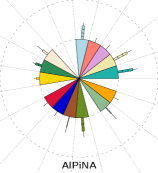
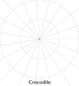
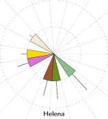

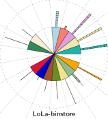
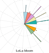
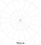

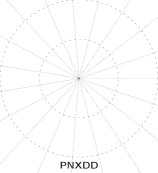
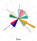

8 RowData for CTL and LTL Formulae Evaluation
No tool participated in these two examinations.
9 Conclusion
This paper reported our experience with the second Model Checking Contest @ Petri nets 2012.
From the tool developers’ point of view, such an event allows to compare tools on a common benchmark that could become a public repository. Also, some mechanisms established for the contest, such as a language to elaborate the formula to be verified could become, over the years, a common way to provide formulæ to the various tools developed by the community.
Some difficulties in the generation of formulæ for the contest led to a very late publication of the grammar. Moreover, it appeared that some difficulties were underestimated for tool integration. This explain why, while the analysis of the state space generation examination is fruitful, this is not the case for the formulæ evaluation ones.
Thus, we provide in this report raw results as they were computed, and with no interpretation, in order to emphasize the effort performed by both the organizers and the tool submitters.
9.0.1 Lesson Learned from MCC’2012
This edition was greatly improved from the lesson learned during the previous edition (see [29]). However, some remarks about the complexity of the submission procedure led to the following suggestions:
-
i
structural formulæ examination will be split in two subcategories: a single request one (asking for deadlock, bound, etc.) and a combined one where these single requests can be combined.
-
ii
for formulaæ examinations, we would like to distinguish satisfied properties from unsatisfied ones. This would provide a better feedback for tool developers (due to the difficulties encountered this year, it was impossible to complete this for the 2012 edition).
-
iii
the structure of a modelscaling value will be simplified, thus avoiding the complex naming problems we encountered this year (especially for fomulæ). This should simplify the integration of model checkers in the image disk.
-
iv
we will provide, as for last year, a pre-installed disk image with a dummy model checker, just to let tool developers see how their tool can be integrated.
-
v
the “surprise model” examination will be processed as well, it is of interest to evaluate the capability of tools with their default settings. We had no time to do so this year.
Finally, we would like to set-up an on-line repository that would help tool developers to submit more models as well as to perform tests on their tools. However, this task requiring more manpower, we do not know if it will be operated for MCC’2013.
9.0.2 Acknowledgements
The Model Checking Contest @ Petri nets organizers would like to thank the following people for the help they provided in setting up this event: Nicolas Gibelin (infrastructure and cluster management), Emmanuel Paviot-Adet and Alexis Marechal (description of selected models), and Steve Hostettler (definition of properties).
The Model Checking Contest organizers would also like to thank the tool developers who made possible such a contest. They are:
-
•
AlPiNA: Steve Hostettler, Alexis Marechal, and Edmundo Lopez;
-
•
Crocodile: Maximilien Colange;
-
•
Helena: Sami Evangelista and Jean-François Pradat-Peyre.
-
•
ITS-Tools: Yann Thierry-Mieg;
-
•
LoLa-binstore and LoLa-bloom: Karsten Wolf;
-
•
Marcie: Alexey Tovchigrechko, Martin Schwarick, and Christian Rohr;
-
•
Neco: Lukasz Fronc;
-
•
PNXDD: Silien Hong and Emmanuel Paviot-Adet;
-
•
Sara: Harro Wimmel and Karsten Wolf.
References
- [1] Aloul, F.A., Markov, I.L., Sakallah, K.A.: FORCE: a fast and easy-to-implement variable-ordering heuristic. In: ACM Great Lakes Symposium on VLSI. pp. 116–119. ACM (2003)
- [2] Behnel, S., Bradshaw, R., Seljebotn, D.: Cython – C extensions for Python. http://www.cython.org
- [3] Buchs, D., Hostettler, S.: Sigma Decision Diagrams. In: Preliminary proceedings of the 5th International Workshop on Computing with Terms and Graphs. pp. 18–32. No. TR-09-05 in TERMGRAPH workshops, Università di Pisa (2009)
- [4] Buchs, D., Hostettler, S., Marechal, A., Risoldi, M.: AlPiNA: An Algebraic Petri Net Analyzer. In: Tools and Algorithms for the Construction and Analysis of Systems, LNCS, vol. 6015, pp. 349–352. Springer (2010)
- [5] Chen, A., Buchs, D., Lucio, L., Pedro, L., Risoldi, M.: Modeling distributed systems using concurrent object oriented petri nets. In: 4th International Workshop on Modelling of Objects, Components and Agents (MOCA). pp. 103–122 (2006)
- [6] Chiola, G., Dutheillet, C., Franceschinis, G., Haddad, S.: On well-formed coloured nets and their symbolic reachability graph. In: Jensen, K., Rozenberg, G. (eds.) Procedings of the 11th International Conference on Application and Theory of Petri Nets (ICATPN’90). Reprinted in High-Level Petri Nets, Theory and Application. Springer-Verlag (1991)
- [7] Chiola, G., Dutheillet, C., Franceschinis, G., Haddad, S.: A symbolic reachability graph for coloured Petri nets. Theoretical Computer Science 176(1–2), 39–65 (1997), citeseer.ist.psu.edu/chiola97symbolic.html
- [8] Chiola, G., Franceschinis, G.: Colored GSPN Models and Automatic Symmetry Detection. In: Petri Nets and Performance Models, The Proceedings of the Third International Workshop, PNPM ’89. pp. 50–60. IEEE Computer Society (1989)
- [9] Choppy, C., Dedova, A., Evangelista, S., Hong, S., Klai, K., Petrucci, L.: The NEO Protocol for Large-Scale Distributed Database Systems: Modelling and Initial Verification. In: 31st International Conference on Petri Nets and Other Models of Concurrency (ICATPN 2010). LNCS, vol. 6128, pp. 145–164. springer (2010), moVe INT LIP6
- [10] Ciardo, G.: Advances in compositional approaches based on kronecker algebra: Application to the study of manufacturing systems. In: 3rd International Workshop on Performability Modeling of Computer and Communication Systems. pp. 61–65 (1996)
- [11] Ciardo, G., Trivedi, K.: A decomposition approach for stochastic reward net models. Perf. Eval 18, 37–59 (1993)
- [12] Ciardo, G., Lüttgen, G., Siminiceanu, R.: Efficient Symbolic State-Space Construction for Asynchronous Systems. In: Application and Theory of Petri Nets 2000, LNCS, vol. 1825, pp. 103–122. Springer Berlin / Heidelberg (2000)
- [13] Clarke, E., Grumberg, O., Jha, S., Lu, Y., Veith, H.: Counterexample-guided abstraction refinement. In: Proc. CAV (2000)
- [14] Colange, M., , Hillah, L.M., Kordon, F., Parutto, P.: Extreme Symmetries in Complex Distributed Systems: the Bag-Oriented Approach. In: Development, Operation and Management of Large-Scale Complex IT Systems, 17th Monterey Workshop, Revised Selected Papers. Lecture Notes in Computer Science, vol. 7539, pp. 330–352. Springer, Oxford, UK (2012)
- [15] Colange, M., Baarir, S., Kordon, F., Thierry-Mieg, Y.: Crocodile: a Symbolic/Symbolic tool for the analysis of Symmetric Nets with Bag. In: 32nd International Conference on Petri Nets and Other Models of Concurrency (ICATPN 2011). LNCS, vol. 6709, pp. 338–347. Springer, Newcastle, UK (June 2011)
- [16] Couvreur, J.M., Thierry-Mieg, Y.: Hierarchical Decision Diagrams to Exploit Model Structure. In: 25th IFIP WG 6.1 International Conference on Formal Techniques for Networked and Distributed Systems (FORTE’05). LNCS, vol. 3731, pp. 443–457. Springer (2005)
- [17] Dasgupta, S., Yakovlev, A.: Modeling and verification of globally asynchronous and locally synchronous ring architectures. In: Design, Automation and Test in Europe Conference and Exposition (DATE). pp. 568–569. IEEE Computer Society (2005)
- [18] Dijkstra, E.W.: Self-stabilizing systems in spite of distributed control. Commun. ACM 17(11), 643–644 (1974)
- [19] Evangelista, S.: High Level Petri Nets Analysis with Helena. In: 26th International Conference on Petri Nets and Other Models of Concurrency (ICATPN 2011). vol. 3536, pp. 455–464 (2005)
- [20] Fronc, L., Pommereau, F.: Optimizing the Compilation of Petri Net Models. In: Proc. of SUMo’11. vol. 726. CEUR (2011)
- [21] Haddad, S., Kordon, F., Petrucci, L., Pradat-Peyre, J.F., Trèves, N.: Efficient State-Based Analysis by Introducing Bags in Petri Net Color Domains. In: 28th American Control Conference (ACC’09). pp. 5018–5025. Omnipress IEEE, St-Louis, USA (June 2009)
- [22] Hamez, A., Thierry-Mieg, Y., Kordon, F.: Building efficient model checkers using hierarchical set decision diagrams and automatic saturation. Fundamenta Informaticae 94(3-4), 413–437 (September 2009)
- [23] Heiner, M., Gilbert, D., Donaldson, R.: Petri nets for systems and synthetic biology. In: 8th International School on Formal Methods for the Design of Computer - SFM 2008. LNCS, vol. 5016, pp. 215–264. Springer (2008)
- [24] Hong, S., Kordon, F., Paviot-Adet, E., Evangelista, S.: Computing a Hierarchical Static order for Decision Diagram-Based Representation from P/T Nets. ToPNoC: Transactions on Petri Nets and Other Models of Concurrency V (2012)
- [25] Hostettler, S., Marechal, A., Linard, A., Risoldi, M., Buchs, D.: High-Level Petri Net Model Checking with AlPiNA. Fundamenta Informaticae 113 (2011)
- [26] ISO/IEC: Software and Systems Engineering - High-level Petri Nets, Part 2: Transfer Format, International Standard ISO/IEC 15909 (February 2011)
- [27] ISO/IEC/JTC1/SC7/WG19: The Petri Net Markup Language home page. http://www.pnml.org (last visited in 2012)
- [28] Jorgensen, J., Kristensen, L.: Computer aided verification of Lamport’s fast mutual exclusion algorithm using colored Petri nets and occurrence graphs with symmetries. IEEE Transactions on Parallel and Distributed Systems 10(7), 714–732 (1999)
- [29] Kordon, F., Linard, A., Buchs, D., Colange, M., Evangelista, S., Lampka, K., Lohmann, N., Paviot-Adet, E., Thierry-Mieg, Y., Wimmel, H.: Report on the Model Checking Contest at Petri Nets 2011. Transactions on Petri Nets and Other Models of Concurrency (ToPNoC) VI (march 2012)
- [30] Kordon, F., Linard, A., Paviot-Adet, E.: Optimized Colored Nets Unfolding. In: 26th International Conference on Formal Methods for Networked and Distributed Systems (FORTE’06). LNCS, vol. 4229, pp. 339–355. Springer, Paris, France (September 2006)
- [31] Krakoviak, S.: Principles of Operating Systems. MIT Press (1988)
- [32] Kristensen, L.M., Schmidt, K., Valmari, A.: Question-guided Stubborn Set Methods for State Properties. Formal Methods in System Design 29(3), 215–251 (2006)
- [33] Linard, A., Paviot-Adet, E., Kordon, F., Buchs, D., Charron, S.: polyDD: Towards a Framework Generalizing Decision Diagrams. In: 10th International Conference on Application of Concurrency to System Design (ACSD’2010). pp. 124–133. IEEE Computer Society, Braga, Portugal (June 2010)
- [34] Linard, A.: Property manual, http://mcc.lip6.fr/2012/pdf/property-manual.pdf. Tech. rep. (2012)
- [35] Peterson, G.L.: Myths about the mutual exclusion problem. Inf. Process. Lett. 12(3), 115–116 (1981)
- [36] Pommereau, F.: SNAKES is the net algebra kit for editors and simulators. http://www.ibisc.univ-evry.fr/~fpommereau/snakes.htm
- [37] Python Software Foundation: Python programming language. http://www.python.org
- [38] Reisig, W.: Elements of Distributed Algorithms. Springer (1998)
- [39] Schmidt, K.: Narrowing petri net state spaces using the state equation. Fundamenta Informaticae 47 (3-4), 325–335 (2001)
- [40] Schmidt, K.: Stubborn sets for standard properties. In: 20th International Conference on Applications and Theory of Petri Nets (ICATPN’99). LNCS, vol. 1639, pp. 46–65. Springer (1999)
- [41] Schwarick, M., Rohr, C., Heiner, M.: MARCIE - Model checking And Reachability analysis done effiCIEntly. In: Proc. 8th International Conference on Quantitative Evaluation of SysTems (QEST 2011). pp. 91 – 100. IEEE CS Press (September 2011)
- [42] Schwarick, M., Tovchigrechko, A.: IDD-based model validation of biochemical networks. TCS 412 pp. 2884–2908 (2010)
- [43] Thierry-Mieg, Y., Ilié, J.M., Poitrenaud, D.: A symbolic symbolic state space representation. In: 24th IFIP WG 6.1 International Conference on Formal Techniques for Networked and Distributed Systems (FORTE’04). LNCS, vol. 3235, pp. 276–291. Springer (2004)
- [44] Thierry-Mieg, Y., Poitrenaud, D., Hamez, A., Kordon, F.: Hierarchical Set Decision Diagrams and Regular Models. In: 15th International Conference on Tools and Algorithms for the Construction and Analysis of Systems (TACAS’09). LNCS, vol. 5505, pp. 1–15. Springer (2009)
- [45] Tovchigrechko, A.: Model Checking Using Interval Decision Diagrams. Ph.D. thesis, BTU Cottbus, Dep. of CS (2008)
- [46] Wikipedia: Dining philosophers problem, http://en.wikipedia.org/wiki/Dining_philosophers_problem (checked in 2012)
- [47] Wikipedia: Sieve of eratosthenes, http://en.wikipedia.org/wiki/Sieve_of_Eratosthenes (checked in 2012)
- [48] Wimmel, H., Wolf, K.: Applying CEGAR to the Petri net state equation. In: Tools and Algorithms for the Construction and Analysis of Systems, 17th International Conference, TACAS 2011. LNCS, vol. 6605, pp. 224–238. Springer (2011)
- [49] Wolf, K.: Generating Petri net state spaces. In: 28th International Conference on Applications and Theory of Petri Nets and Other Models of Concurrency. LNCS, vol. 4546, pp. 29–42. Springer (Jun 2007)