Reducing the size and number of linear programs in a dynamic Gröbner basis algorithm

Abstract.

The dynamic algorithm to compute a Gröbner basis is nearly twenty years old, yet it seems to have arrived stillborn; aside from two initial publications, there have been no published followups. One reason for this may be that, at first glance, the added overhead seems to outweigh the benefit; the algorithm must solve many linear programs with many linear constraints. This paper describes two methods that reduce both the size and number of these linear programs.

1. Introduction

Since the first algorithm to compute Gröbner bases was described by [6], they have become a standard tool for applied, computational, and theoretical algebra. Their power and promise has stimulated a half-century of research into computing them efficiently. Important advances have resulted from reducing the number of pairs considered [6][7][11][16][24], improving the reduction algorithm [5][15][33], and forbidding some reductions [1][16][34].

The Gröbner basis property depends on the choice of term ordering: a basis can be Gröbner with respect to one term ordering, but not to another. Researchers have studied ways to find an ordering that efficiently produces a basis “suitable” for a particular problem [30][31], and to convert a basis that is Gröbner with respect to one ordering to a basis that is Gröbner with respect to another [10][13][17][32].

Another approach would be to begin without any ordering, but to compute both a basis and an ordering for which that basis is Gröbner. Such a “dynamic” algorithm would change its ordering the moment it detected a “more efficient” path towards a Gröbner basis, and would hopefully conclude with a smaller basis more quickly.

Indeed, this question was posed nearly twenty years ago, and was studied both theoretically and practically in two separate papers [9][21]. The first considered primarily questions of discrete geometry; the dynamic algorithm spills out as a nice application of the ideas, but the authors did not seriously consider an implementation. The second described a study implementation that refines the ordering using techniques from linear programming, and focused on the related algebraic questions.

Aside from one preprint [20], there has been no continuation of this effort. There certainly are avenues for study; for example, this observation at the conclusion of [9]:

In a number of cases, after some point is reached in the refining of the current order, further refining is useless, even damaging. …The exact determination of this point is not easy, and an algorithm for its determination is not given.

An example of the damage that can occur is that the number and size of the linear programs grow too large. The temporary solution of [9] was to switch the refiner off at a predetermined point. Aside from the obvious drawback that this prevents useful refinement after this point, it also forces unnecessary refinement before it! This can be especially costly when working with systems rich in dense polynomials.

This paper presents two new criteria that signal the refiner not only to switch off when it is clearly not needed, but also to switch back on when there is a high probability of useful refinement. The criteria are based on simple geometric insights related to linear programming. The practical consequence is that these techniques reduce both the number and the size of the associated linear programs by significant proportions.

2. Background

This section lays the groundwork for what is to follow, in terms of both terminology and notation. We have tried to follow the vocabulary and notation of [9], with some modifications.

Section 2.1 reviews the traditional theory of Gröbner bases, inasmuch as it pertains to the (static) Buchberger algorithm. Section 2.2 describes the motivation and background of the dynamic algorithm, while Section 2.3 reviews Caboara’s specification. Section 2.4 deals with some geometric considerations which will prove useful later.

2.1. Gröbner bases and the static Buchberger algorithm

Let $m,n\in\mathbb{N}^{+}$, $K$ a field, and $R=\mathbb{F}\left[x_{1},\ldots,x_{n}\right]$. We typically denote polynomials by $f$, $g$, $h$, $p$, $q$, and $r$, and the ideal of $R$ generated by any $F\subseteq R$ as $\left<F\right>$. Following [9], we call a product of powers of the variables of $R$ a term, and a product of a term and an element of $K$ a monomial. We typically denote constants by letters at the beginning of the alphabet, and terms by $t$, $u$, $v$. We denote the exponent vector of a term by its name in boldface; so, if $n=4$ and $t=x_{1}^{2}x_{3}x_{4}^{20}$, then $\mathbf{t}=\left(2,0,1,20\right)$.

An ordering $\sigma$ on the set $\mathbb{T}^{n}$ of all terms of $R$ is admissible if it is a well-ordering that is compatible with divisibility and multiplication; by “compatible with divisibility,” we mean that $t\mid u$ and $t\neq u$ implies that $t<_{\sigma}u$, and by “compatible with multiplication,” we mean that $t<_{\sigma}u$ implies that $tv<_{\sigma}uv$. We consider only admissible orderings, so henceforth we omit the qualification.

We write $\mathcal{T}$ for the set of all term orderings, and denote orderings by Greek letters $\mu$, $\sigma$, and $\tau$. For any $p\in R$ we write $\mathrm{lt}_{\sigma}\left(p\right)$ and $\mathrm{lc}_{\sigma}\left(p\right)$ for the leading term and leading coefficient of $p$ with respect with $\sigma$. If the value of $\sigma$ is clear from context or does not matter, we simply write $\mathrm{lt}\left(p\right)$ and $\mathrm{lc}\left(p\right)$. For any $F\subseteq R$, we write $\mathrm{lt}_{\sigma}\left(F\right)=\left\{\mathrm{lt}_{\sigma}\left(f\right):f\in F\right\}$.

Let $I$ be an ideal of $R$, and $G\subseteq I$. If for every $p\in I$ there exists $g\in G$ such that $\mathrm{lt}\left(g\right)\mid\mathrm{lt}\left(p\right)$, then we say that $G$ is a Gröbner basis of $I$. This property depends on the ordering; if $\sigma,\tau\in\mathcal{T}$, it is quite possible for $G$ to be a Gröbner basis with respect to $\sigma$, but not with respect to $\tau$.

It is well known that every polynomial ideal has a finite Gröbner basis, regardless of the choice of ordering. Actually computing a Gröbner basis requires a few more concepts. Let $f,p,r\in R$. We say that $p$ reduces to r modulo $f$, and write $p\underset{f}{\longrightarrow}r$, if there exist $a\in K$ and $t\in\mathbb{T}^{n}$ such that $p-atf=r$ and $\mathrm{lt}\left(r\right)<\mathrm{lt}\left(p\right)$. Similarly, we say that $p$ reduces to $r$ modulo $G$, and write

$$p\underset{G}{\longrightarrow}r,$$

if there exist $\left\{i_{1},\ldots,i_{\ell}\right\}\subseteq\left\{1,\ldots,\#G\right\}$ such that $p\underset{g_{i_{1}}}{\longrightarrow}r_{1}$, $r_{1}\underset{g_{i_{2}}}{\longrightarrow}r_{2}$, …, $r_{\ell-1}\underset{g_{i_{\ell}}}{\longrightarrow}r_{\ell}=r$. If there no longer exists $g\in G$ such that $\mathrm{lt}\left(g\right)$ divides a $\mathrm{lt}\left(r\right)$, we call $r$ a remainder of $p$ modulo $G$.

Proposition 1 (Buchberger’s Characterization, [6]).

$G$ is a Gröbner basis of $I$ if and only if the S-polynomial of every $f,g\in I\backslash\left\{0\right\}$, or

$$\mathrm{spoly}\left(f,g\right)=\mathrm{lc}\left(g\right)\cdot\frac{\mathrm{lcm}\left(\mathrm{lt}\left(f\right),\mathrm{lt}\left(g\right)\right)}{\mathrm{lt}\left(f\right)}\cdot f-\mathrm{lc}\left(f\right)\cdot\frac{\mathrm{lcm}\left(\mathrm{lt}\left(f\right),\mathrm{lt}\left(g\right)\right)}{\mathrm{lt}\left(g\right)}\cdot g,$$

reduces to zero modulo $G$.

For convenience, we extend the definition of an $S$-polynomial to allow for $0$:

Definition 2.

Let $p\in R$. The S-polynomial of $p$ and $0$ is $p$.

Buchberger’s Characterization of a Gröbner basis leads naturally to the classical, static Buchberger algorithm to compute a Gröbner basis; see Algorithm 2.1, which terminates on account of the Hilbert Basis Theorem (applied to $\left<\mathrm{lt}\left(G\right)\right>$). There are a number of ambiguities in this algorithm: the strategy for selecting pairs $\left(p,q\right)\in P$, for instance, or how precisely to reduce the $S$-polynomials. These questions have been considered elsewhere, and the interested reader can consult the references cited in the introduction.

 

algorithm static_buchberger_algorithm

inputs:

• $F\subseteq R$

• $\sigma\in\mathcal{T}$

outputs: $G\subseteq R$, a Gröbner basis of $\left<F\right>$ with respect to $\sigma$

do:

1. Let $G=\left\{\right\}$, $P=\left\{\left(f,0\right):f\in F\right\}$

2. while $P\neq\emptyset$

   1. Select $\left(p,q\right)\in P$ and remove it

   2. Let $r$ be a remainder of $\mathrm{spoly}\left(p,q\right)$ modulo $G$

   3. if $r\neq 0$

      1. Add $\left(g,r\right)$ to $P$ for each $g\in G$

      2. Add $r$ to $G$

3. return $G$

Figure 2.1. The traditional Buchberger algorithm

 

Remark 3.

Algorithm 2.1 deviates from the usual presentation of Buchberger’s algorithm by considering $S$-polynomials of the inputs with 0, rather than with each other. This approach accommodates the common optimization of interreducing the inputs.

2.2. The dynamic algorithm

Every admissible ordering can be described using a real matrix $M$ [26]. Terms $u,v$ are compared by comparing lexicographically $M\mathbf{u}$ and $M\mathbf{v}$. Two well-known orders are lex and grevlex; the former can be represented by an identity matrix, and the latter by an upper-triangular matrix whose non-zero elements are identical.

Example 4.

Consider the well-known Cyclic-4 system,

$$F =\left(x_{1}+x_{2}+x_{3}+x_{4},x_{1}x_{2}+x_{2}x_{3}+x_{3}x_{4}+x_{4}x_{1},\right.$$

$$\phantom{=(x_{1}}x_{1}x_{2}x_{3}+x_{2}x_{3}x_{4}+x_{3}x_{4}x_{1}+x_{4}x_{1}x_{2},$$

$$\left.\phantom{=(x_{1}}x_{1}x_{2}x_{3}x_{4}-1\right).$$

1. If we compute a Gröbner basis of $\left<F\right>$ with respect to lex, we obtain a Gröbner basis with 6 polynomials made up of 18 distinct terms.

2. If we compute a Gröbner basis of $\left<F\right>$ with respect to grevlex, we obtain a Gröbner basis with 7 polynomials made up of 24 distinct terms.

3. If we compute a Gröbner basis of $\left<F\right>$ according to the matrix ordering

   $$\left(\begin{array}[]{cccc}1&3&2&4\\ 1&1&1&0\\ 1&1&0&0\\ 1&0&0&0\end{array}\right),$$

   we obtain a Gröbner basis with 5 polynomials and 19 distinct terms.

We can order any finite set of terms using a weight vector in $\mathbb{N}^{n}$, and if necessary, we can extend a weight vector to an admissible ordering by adding $n-1$ linearly independent rows. In the example above, we extended the weight vector $\left(1\;3\;2\;4\right)$ by adding three more rows.

The goal of the dynamic algorithm is to discover a “good” ordering for given input polynomials during the Gröbner basis computation. Algorithm 2.2 describes a dynamic Buchberger algorithm. As with the static algorithm, its basic form contains a number of unresolved ambiguities:

 

algorithm dynamic_buchberger_algorithm

inputs: $F\subseteq R$

outputs: $G\subseteq R$ and $\sigma\in\mathcal{T}$ such that $G$ is a Gröbner basis of $\left<F\right>$ with respect to $\sigma$

do:

1. Let $G=\left\{\right\}$, $P=\left\{\left(f,0\right):f\in F\right\}$, $\sigma\in\mathcal{T}$

2. while $P\neq\emptyset$

   1. Select $\left(p,q\right)\in P$ and remove it

   2. Let $r$ be a remainder of $\mathrm{spoly}\left(p,q\right)$ modulo $G$

   3. if $r\neq 0$

      1. Add $\left(g,r\right)$ to $P$ for each $g\in G$

      2. Add $r$ to $G$

   4. Select $\tau\in\mathcal{T}$

   5. Let $P=P\cup\left\{\left(p,q\right):p,q\in G,\;p\neq q,\;\mathrm{lt}_{\sigma}\left(p\right)\neq\mathrm{lt}_{\tau}\left(p\right)\right\}$

   6. Let $\sigma=\tau$

3. return $G$, $\sigma$

Figure 2.2. A basic, dynamic Buchberger algorithm

 

• How shall we select a pair?

• How do we determine a good ordering?

• How do we choose the ordering?

• When should we select a new ordering?

• Does the algorithm actually terminate?

2.3. Caboara’s implementation

The only implementation of a dynamic algorithm up to this point was that of [9]; it has since been lost. This section reviews that work, adapting the original notation to our own, though any differences are quite minor.

2.3.1. How shall we select a pair?

Caboara used the sugar strategy, which selects $\left(p,q\right)\in P$ such that the degree of the homogenization of $\mathrm{spoly}\left(p,q\right)$ is minimal [4][19]. Pairs were pruned using the Gebauer-Möller algorithm [18].

2.3.2. How do we determine a good ordering?

Both [21, 9] suggest using the Hilbert-Poincaré function to evaluate orderings. Roughly speaking, the Hilbert-Poincaré function of an ideal $I$ in a ring $R$, denoted $H_{R/I}\left(d\right)$, indicates:

• if $I$ is inhomogeneous, the number of elements in $R/I$ of degree no greater than $d$;

• if $I$ is homogeneous, the number of elements in $R/I$ of degree $d$.

The homogeneous case gives us the useful formula

$$H_{R/I}\left(d\right)=\dim_{K}\left(R/I\right)_{d},$$

where the dimension is of the subspace of degree-$d$ terms of the vector space $R/I$. If $G$ is a Gröbner basis, then $H_{R/\left<G\right>}=H_{R/\left<\mathrm{lt}\left(G\right)\right>}$, and it is easy to compute the related Hilbert series or Hilbert polynomial for $H_{R/\left<G\right>}\left(d\right)$ from $\left<\mathrm{lt}\left(G\right)\right>$ [2][3][27]. Many textbooks, such as [23], contain further details.

In the homogeneous setting, the Hilbert function is an invariant of the ideal regardless of the ordering. Thus, we can use it to measure “closeness” of a basis to a Gröbner basis. Both the static and dynamic algorithms add a polynomial $r$ to the basis $G$ if and only if $\left<\mathrm{lt}\left(G\right)\right>\subsetneq\left<\mathrm{lt}\left(G\cup\left\{r\right\}\right)\right>$. (See Figure 2.3.)

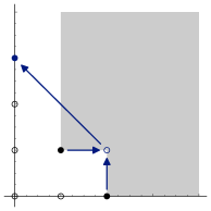
Figure 2.3. Adding $r$ to $G$ makes $R/\left<\mathrm{lt}\left(G\right)\right>$, and therefore $H_{\left<\mathrm{lt}\left(G\right)\right>}$, smaller. The example here is taken from $G=\left\{x^{2}+y^{2}-4,xy-1\right\}$ with $x>y$; running the Buchberger algorithm on the pair $\left(g_{1},g_{2}\right)$ gives us $\mathrm{lt}\left(r\right)=y^{3}$, which removes all multiples of $y^{3}+\left<G\right>$ from $R/\left<G\right>$, thereby decreasing $H_{\left<\mathrm{lt}\left(G\right)\right>}$.

If we denote $T=\left<\mathrm{lt}\left(G\right)\right>$ and $U=\left<\mathrm{lt}\left(G\cup\left\{r\right\}\right)\right>$, then $T\subsetneq U$, so for all $d$,

$$H_{R/T}\left(d\right)=\dim_{K}\left(R/T\right)_{d}\geq\dim_{K}\left(R/U\right)_{d}=H_{R/U}\left(d\right).$$

If the choice of ordering means that we have two possible values for $U$, we should aim for the ordering whose Hilbert function is smaller in the long run.

Since $G$ is a Gröbner basis only once we complete the algorithm, how can we compute the Hilbert function of its ideal? We do not! Instead, we approximate it using a tentative Hilbert function $H_{R/\left<\mathrm{lt}\left(G\right)\right>}\left(d\right)$. This usually leads us in the right direction, even when the polynomials are inhomogeneous [9].

2.3.3. How do we choose the ordering?

A potential leading term (PLT) of $r\in R$ is any term $t$ of $r$ for which there exists an admissible ordering $\sigma$ such that $\mathrm{lt}_{\sigma}\left(r\right)=t$. As long as $G$ is finite, there is a finite set of equivalence classes of all monomial orderings. We call each equivalence class a cone associated to $G$, and denote by $C\left(\sigma,G\right)$ the cone associated to $G$ that contains a specific ordering $\sigma$. When $g\in G$, we refer to $C\left(\sigma,t,g\right)$ as the cone associated to $G$ that guarantees $\mathrm{lt}_{\sigma}\left(g\right)=t$.

Suppose $t\in\mathrm{supp}\left(r\right)$ and we want to choose $\sigma$ such that $\mathrm{lt}_{\sigma}\left(r\right)=t$. For each $u\in\mathrm{supp}\left(r\right)\backslash\left\{t\right\}$, we want $t>u$. This means $\sigma\mathbf{t}>\sigma\mathbf{u}$, or $\sigma\left(\mathbf{t}-\mathbf{u}\right)>0$. A vector will suffice to determine $\sigma$; and we can find such a vector using the system of linear inequalities

$$\mathrm{lp}\left(y,t,r\right)=\left\{y_{k}>0\right\}_{k=1}^{n}\cup\left\{\sum_{k=1}^{n}y_{k}\left(t_{k}-u_{k}\right)>0\right\}_{u\in\mathrm{supp}\left(r\right)\backslash\left\{t\right\}}.$$

(Here, $t_{k}$ and $u_{k}$ denote the $k$th entry of $\mathbf{t}$ and $\mathbf{u}$, respectively. To avoid confusion with the variables of the polynomial ring, we typically use $y$’s to denote the unknown values of linear programs.) Since every cone $C\left(\sigma,G\right)$ is defined by some system of linear inequalities, this approach successfully turns a difficult geometric problem into a well-studied algebraic problem that we can solve using techniques from linear programming.

Proposition 5 (Propositions 1.5, 2.3 of [9]).

The cone $C\left(\sigma,F\right)$ can be described using a union of such systems, one for each $f\in F$.

Example 6.

In Cyclic-4, the choice of leading terms

$$\left\{x_{1},x_{1}x_{2},x_{1}x_{2}x_{3},x_{1}x_{2}x_{3}x_{4}\right\}$$

can be described by the system of linear inequalities

$$\left\{y_{i}>0\right\}_{i=1}^{4} \cup\left\{y_{1}-y_{i}>0\right\}_{i=2}^{4}$$

$$\cup\left\{y_{1}-y_{3}>0,y_{1}+y_{2}-y_{3}-y_{4}>0,y_{2}-y_{4}>0\right\}$$

$$\cup\left\{y_{1}-y_{4}>0,y_{2}-y_{4}>0,y_{3}-y_{4}>0\right\}$$

$$\cup\left\{y_{1}+y_{2}+y_{3}+y_{4}-0>0\right\}.$$

The last inequality comes from the constraint $x_{1}x_{2}x_{3}x_{4}>1$, and is useless. This illustrates an obvious optimization; if $u\mid t$ and $u\neq t$, the ordering’s compatibility with division implies that $u$ cannot be a leading term of $r$; the corresponding linear inequality is trivial, and can be ignored. This leads to the first of two criteria to eliminate terms that are not potential leading terms.

Proposition 7 (The Divisibility Criterion; Proposition 2.5 and Corollary of [9]).

Let $r\in R$ and $t,u\in\mathrm{supp}\left(r\right)$. If $u$ divides $t$ properly, then $t>_{\tau}u$ for every $\tau\in\mathcal{T}$. In other words, $u$ is not a potential leading term of $r$.

Caboara also proposed a second criterion based on the notion of refining the order. If $\sigma$ and $\tau$ are such that $C\left(\tau,G\right)\subseteq C\left(\sigma,G\right)$, then we say that $\tau$ refines $\sigma$, or that $\tau$ refines the order. Caboara’s implementation chooses an ordering $\tau$ in line 2d so that $\mathrm{lt}_{\tau}\left(g\right)=\mathrm{lt}_{\sigma}\left(g\right)$ for all $g\in G\backslash\left\{r\right\}$, so that $\tau$ refines $\sigma$. This allows the algorithm to discard line 2e altogether, and this is probably a good idea in general.

Proposition 8 (The Refining Criterion; Proposition 2.6 of [9]).

Let $G=\left\{g_{1},\ldots,g_{\ell}\right\}\subsetneq R$ and $t_{1},\ldots,t_{\ell}$ be potential leading terms of $g_{1},\ldots,g_{\ell}$, respectively. The system

$$\left\{t_{k}>u:u\in\mathrm{supp}\left(g_{k}\right)\right\}_{k=1}^{\ell}$$

is equivalent to the system

$$\left\{t_{k}>u:u\mbox{ a PLT of }g_{k}\mbox{ consistent w/}t_{j}=\mathrm{lt}\left(g_{j}\right)\;\forall j=1,\ldots,k-1\right\}_{k=1}^{\ell}.$$

Proposition 8 implies that we need only compare $t_{k}$ with other potential leading terms $u$ of $g_{k}$ that are consistent with the previous choices; we will call such $u$, compatible leading terms. From a practical point of view, refining the cone in this way is a good idea, as the technique of refining the order allows one to warm-start the simplex algorithm from a previous solution using the dual simplex algorithm, lessening the overhead of linear programming. It does require some record-keeping; namely, retaining and expanding the linear program as we add new polynomials. This motivates the definition of

$$\mathrm{lp}\left(\sigma,G\right)=\mathrm{lp}\left(\sigma,\left\{\left(\mathrm{lt}_{\sigma}\left(g\right),g\right):g\in G\right\}\right):=\bigcup_{g\in G}\mathrm{lp}\left(y,\mathrm{lt}_{\sigma}\left(g\right),g\right).$$

This burden on space is hardly unreasonable, however, as these systems would have to be computed even if we allow the order to change. That approach would entail a combinatorial explosion.

Example 9.

Let $F$ be the Cyclic-4 system. Suppose that, in the dynamic algorithm, we add $\mathrm{spoly}\left(f_{1},0\right)=f_{1}$ to $G$, selecting $x_{1}$ for the leading term, with $\sigma=\left(2,1,1,1\right)$. Suppose that next we select $\mathrm{spoly}\left(f_{2},0\right)=f_{2}$, reduce it modulo $G$ to $r_{2}=x_{2}^{2}-2x_{2}x_{4}-x_{4}^{2}$, and select $x_{2}^{2}$ as its leading term, with $\sigma=\left(3,2,1,1\right)$. We have

$$\mathrm{lp}\left(\sigma,\left\{\left(x_{1},f_{1}\right),\left(x_{2}^{2},f_{2}\right)\right\}\right) =\phantom{\cup}\left\{y_{k}>0\right\}_{k=1}^{4}\cup\left\{y_{1}-y_{k}>0\right\}_{k=2}^{4}$$

$$\phantom{=\;}\cup\left\{y_{2}-y_{4}>0,2y_{2}-2y_{4}>0\right\}.$$

Remark 10.

In a practical implementation, it is important to avoid redundant constraints; otherwise, the programs quickly grow unwieldy. One way to avoid redundant constraints is to put them into a canonical form that allows us to avoid adding scalar multiples of known constraints. Unfortunately, even this grows unwieldy before too long; one of this paper’s main points is to describe a method of minimizing the number of required constraints.

2.3.4. When should we select the ordering?

As noted in the introduction, Caboara’s implementation refines the ordering for a while, then permanently switches the refiner off. Making this activation/deactivation mechanism more flexible is the major goal of this investigation.

2.3.5. Does the algorithm actually terminate?

Termination is easy to see if you just refine orderings. In the more general case, termination has been proved by Golubitsky [20]. He has found systems where it is advantageous to change the ordering, rather than limit oneself to refinement.

2.4. The geometric point of view

Here, we provide a visual interpretation of how the property $C\left(\tau,G\right)\subsetneq C\left(\sigma,G\right)$ affects the algorithm. This discussion was originally inspired by [21], but we state it here in terms that are closer to the notion of a Gröbner fan [25].

Any feasible solution to the system of linear inequalities corresponds to a half-line in the positive orthant. Thus, the set of all solutions to any given system forms an open, convex set that resembles an infinite cone. Adding polynomials to $G$ sometimes splits some of the cones. (See Figure 2.4). This gives a geometric justification for describing Caboara’s approach as a narrowing cone algorithm.

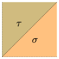
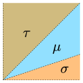
Figure 2.4. The cones associated to a basis $G$ narrow as we add polynomials to the basis. Here, $G=\left\{x^{2}+y^{2}-4,xy-1\right\}$; the two possible orderings are $\tau$ and $\sigma$, which give $\mathrm{lt}_{\sigma}\left(G\right)=\left\{x^{2},xy\right\}$ and $\mathrm{lt}_{\tau}\left(G\right)=\left\{y^{2},xy\right\}$. Suppose we choose $\sigma$ and compute the $S$-polynomial. This adds $r=y^{3}+x-4y$ to the basis, and the cone containing $\sigma$ splits, giving us two choices for $\mathrm{lt}\left(r\right)$.

Even though some cones can split when we add new polynomials, not all clones must split. In particular, the cone containing the desired ordering need not split, especially when the algorithm is nearly complete. For this, reason, it is not necessary to refine the cone every time a polynomial is added. The methods of the next section help detect this situation.

3. Exploiting the narrowing cone

The main contribution of this paper is to use the narrowing cone to switch the refiner on and off. We propose two techniques to accomplish this: one keeps track of cones known to be disjoint (Section 3.1); the other keeps track of “boundary vectors” that prevent the refiner from leaving the cone (Section 3.2).

3.1. Disjoint Cones

The Disjoint Cones Criterion is based on the simple premise that if we track inconsistent constraints of linear programs, we can avoid expanding the program later.

3.1.1. Geometric motivation

Let

• $C_{T}$ be the cone defined by the selection of $T=\left\{t_{1},\ldots,t_{\ell}\right\}$ as the leading terms of $G=\left\{g_{1},\ldots,g_{\ell}\right\}$,

• $C_{u}$ be the cone defined by the selection of $u$ as the leading term of $g_{\ell+1}$, and

• $C_{T^{\prime}}$ be the cone defined by the selection of $T^{\prime}=\left\{t_{1},\ldots,t_{\ell+k}\right\}$ as the leading terms of $G^{\prime}=\left\{g_{1},\ldots,g_{\ell+k}\right\}$.

Suppose the current ordering is $\sigma\in C_{T}$, and $C_{T}\cap C_{u}=\emptyset$. It is impossible to refine the current ordering in a way that selects $u$ as the leading term of $g_{\ell+1}$, as this would be inconsistent with previous choices. On the other hand, if $\tau\in C_{T^{\prime}}$ and $C_{T^{\prime}}\subseteq C_{T}$, then it is possible to refine $\sigma$ to an ordering $\tau$.

Now let

• $C_{v}$ be the cone defined by the selection of $v$ as the leading term for $g_{\ell+k+1}$.

If $C_{v}\subseteq C_{u}$, then $C_{v}\cap C_{T^{\prime}}\subseteq C_{u}\cap C_{T}=\emptyset$, so we cannot refine $\sigma$ to any ordering that selects $v$ as the leading term of $g_{\ell+k+1}$. Is there some way to ensure that the algorithm does not waste time solving such systems of linear inequalities? Yes! If we record the cone $C_{u}$, we can check whether $C_{v}\subseteq C_{u}$, rather than going to the expense of building a linear program to check whether $C_{v}\cap C_{T^{\prime}}\neq\emptyset$.

3.1.2. Algebraic implementation

We could determine whether $C_{v}\subseteq C_{u}$ by building a linear program, but we will content ourselves with determining when one set of inconsistent linear constraints is a subset of another set.

Theorem 11 (Disjoint Cones Criterion).

Let $L_{T}$, $L_{U}$, and $L_{V}$ be sets of linear constraints. If $L_{T}$ is inconsistent with $L_{U}$ and $L_{U}\subseteq L_{V}$, then $L_{T}$ is also inconsistent with $L_{V}$.

Proof.

Assume $L_{T}$ is inconsistent with $L_{U}$ and $L_{U}\subseteq L_{V}$. The first hypothesis implies that $L_{T}\cap L_{U}=\emptyset$. The second implies that $L_{V}$ has at least as many constraints as $L_{U}$, so that the feasible regions $C_{U}$ and $C_{V}$, corresponding to $L_{U}$ and $L_{V}$, respectively, satisfy the relation $C_{U}\supseteq C_{V}$. Putting it all together, $C_{V}\cap C_{T}\subseteq C_{U}\cap C_{T}=\emptyset$. ∎

In our situation, $L_{U}$ and $L_{V}$ correspond to different choices of leading terms of a new polynomial added to the set, while $L_{T}=\mathrm{lp}\left(\sigma,G\right)$. We want to consider both the case where $L_{V}$ is a set of new constraints, and the case where $L_{V}$ is some extension of $L_{T}$. Rather than discard the inconsistent linear program $L_{U}$, we will retain it and test it against subsequent sets of constraints, avoiding pointless invocations of the simplex algorithm.

We implement the geometric idea using a global variable, $\mathit{rejects}$. This is a set of sets; whenever $L_{T}$ is known to be consistent, but the simplex algorithm finds $L_{T}\cup L_{U}$ inconsistent, we add $L_{U}$ to $\mathit{rejects}$. Subsequently, while creating the constraints in an extension $L_{V}$ of $L_{T}$, we check whether $L_{U}$ is contained in either $L_{V}$ or $L_{T}\cup L_{V}$; if so, we reject $L_{V}$ out of hand, without incurring the burden of the simplex algorithm.

Again, we are not checking whether the cones are disjoint, only the necessary condition of whether the linear constraints are a subset. With appropriate data structures, the complexity of determining subset membership is relatively small; with hashed sets, for example, the worst-case time complexity would be the cost of the hash function plus $O\left(\left|\mathit{rejects}\right|\right)$.

3.2. Boundary Vectors

Unlike the Disjoint Cones Criterion, the Boundary Vectors Criterion can prevent the construction of any constraints.

3.2.1. Geometric motivation

Let $C\left(G,\sigma\right)$ be a cone associated with $G$, containing the ordering $\sigma$.

Definition 12.

The closure of $C\left(G,\sigma\right)$ is the feasible region obtained by rewriting $\mathrm{lp}\left(\sigma,G\right)$ as inclusive inequalities ($\geq$ in place of $>$). Let $d\in\mathbb{R}$ be positive. We say that $\omega\in\mathbb{R}^{n}$ is a boundary vector of $C\left(G,\sigma\right)$ if it is an extreme point of the intersection of the closure of $C\left(G,\sigma\right)$ and the additional constraint $\sum_{k=1}^{n}x_{k}=d$.

For a fixed $d$, we denote the set of all boundary vectors of $C\left(G,\sigma\right)$ by $\Omega_{G,\sigma,d}$. When the value of $d$ is not critical to the discussion, we simply write $\Omega_{G,\sigma}$. Likewise, if the values of $G$ and $\sigma$ are not critical to the discussion, or if they are understood from context, we simply write $\Omega$.

Example 13.

Suppose $\sigma=\left(18,5,7\right)$ and $C\left(G,\sigma\right)$ is defined by

$$\left\{\begin{array}[]{rl}2y_{1}-y_{2}&>0\\ -y_{1}+4y_{2}&>0\\ y_{1}+y_{2}-3y_{3}&>0\\ -y_{2}+y_{3}&>0\end{array}\right..$$

When $d=30$, we have $\Omega=\left\{\left(15,7.5,7.5\right),\left(20,5,5\right),\left(18,4.5,7.5\right)\right\}$. Not all intersections of constraints are boundary vectors; one intersection that does not border the feasible region is $\left(22.5,0,7.5\right)$, which satisfies all but the third constraint.

Boundary vectors possess the very desirable property of capturing all possible refinements of the term ordering.

Theorem 14 (Boundary Vectors Criterion).

Let $r\in R$ and $\Omega$ the set of boundary vectors of $C\left(\sigma,G\right)$. Write $t=\mathrm{lt}_{\sigma}\left(r\right)$. If there exists $\tau\in C\left(\sigma,G\right)$ such that $\mathrm{lt}_{\tau}\left(r\right)=u\neq t$ — that is, there exists $\tau$ that refines the order differently from $\sigma$ — then there exists $\omega\in\Omega$ such that $\omega\left(\mathbf{u}-\mathbf{t}\right)>\mathbf{0}$.

Two observations are in order before we prove Theorem 14. First, the converse of Theorem 14 is not true in general. For example, let $\omega=\left(2,1\right)$, $r=x^{2}+x+y$, $v=x^{2}$, $u=x$, and $t=y$. Even though $\omega\left(\mathbf{u}-\mathbf{t}\right)>0$, the fact that $u\mid v$ implies that no admissible ordering $\tau$ chooses $\mathrm{lt}_{\tau}\left(r\right)=u$.

Nevertheless, the theorem does imply a useful corollary:

Corollary 15.

If we know the set $\Omega$ of boundary vectors for $C\left(\sigma,G\right)$, then we can discard any term $u$ such that $\omega\left(\mathbf{t}-\mathbf{u}\right)>0$ for all $\omega\in\Omega$. That is, $u$ is not a compatible leading term.

We turn now to the proof of Theorem 14. Figure 3.1 illustrates the intuition;

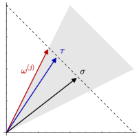
Figure 3.1. If $\mathrm{lt}_{\tau}\left(r\right)\neq\mathrm{lt}_{\sigma}\left(r\right)$, convexity and linearity imply that we can find a boundary vector $\omega$ such that $\omega$ would give $\mathrm{lt}_{\tau}\left(r\right)$ more weight than $\mathrm{lt}_{\sigma}\left(r\right)$.

here, $\tau$ and $\sigma$ select different leading terms, and $\omega$ lies on the other side of $\tau$ from $\sigma$. By linearity, $\omega$ gives greater weight to $\mathrm{lt}_{\tau}\left(r\right)$ than to $\mathrm{lt}_{\sigma}\left(r\right)$.

of Theorem 14.

Suppose that there exists $\tau\in C\left(\sigma,G\right)$ such that $\mathrm{lt}_{\tau}\left(r\right)=u$. By definition, $\tau\left(\mathbf{u}-\mathbf{t}\right)>0$. Let $d=\sum\tau_{k}$; if $\tau=\omega$ for some $\omega\in\Omega_{G,\sigma,d}$, then we are done. Otherwise, consider the linear program defined by maximizing the objective function $\sum y_{k}\left(u_{k}-t_{k}\right)$ subject to the closure of $\mathrm{lp}\left(\sigma,G\right)\cup\left\{\sum y_{k}=\sum\tau_{k}\right\}$. This is a convex set; the well-known Corner Point Theorem implies that a maximum of any objective function occurs at an extreme point [12][29]. By definition, such a point is a boundary vector of $C\left(\sigma,G\right)$. Let $\omega\in C\left(\sigma,G\right)$ be a boundary vector where $\sum y_{k}\left(u_{k}-t_{k}\right)$ takes its maximum value; then $\omega\left(\mathbf{u}-\mathbf{t}\right)\geq\tau\left(\mathbf{u}-\mathbf{t}\right)>0$. ∎

Computing $\Omega$ can be impractical, as it is potentially exponential in size. We approximate it instead by computing corner points that correspond to the maximum and minimum of each variable on a cross section of the cone with a hyperplane, giving us at most $2n$ points. Figure 3.2

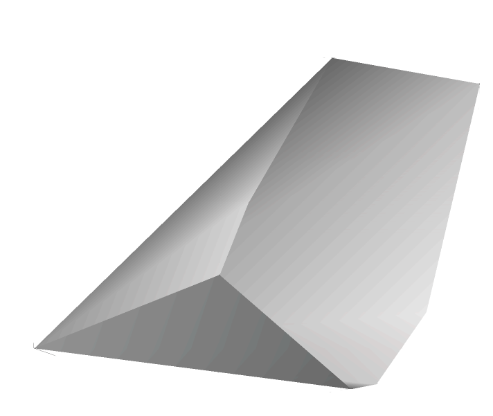
Figure 3.2. We approximate $\Omega$ by computing boundary vectors corresponding to points that maximize and minimize the value of an objective function. The cone at the left has seven boundary vectors, as we see in the cross section on the right. In this case, four vectors maximize and minimize the variables; they define a “sub-cone” whose cross-section corresponds to the dashed line.

illustrates the idea.

Example 16.

Continuing Example 13, maximizing $y_{1}$, $y_{2}$, and $y_{3}$ gives us the boundary vectors listed in that example. In this case, these are all the boundary vectors, but we are not always so lucky.

Approximating $\Omega$ has its own disadvantage; inasmuch as some orderings are excluded, we risk missing some refinements that could produce systems that we want. We will see that this is not a serious drawback in practice.

3.2.2. Minimizing the number of constraints

While boundary vectors reduce the number of linear programs computed, the size of the linear programs can remain formidable. After all, we are still adding constraints for every monomial that passes the Divisibility Criterion. Is there some way to use boundary vectors to minimize the number of constraints in the program?

We will attempt to add only those constraints that correspond to terms that the boundary vectors identify as compatible leading terms. As we are not computing all the boundary vectors, the alert reader may wonder whether this is safe.

Example 17.

Suppose

• $\mu\in C\left(\tau,\left\{g_{1},\ldots,g_{\ell+k}\right\}\right)\subsetneq C\left(\sigma,\left\{g_{1},\ldots,g_{\ell}\right\}\right)$,

• $t=\mathrm{lt}_{\sigma}\left(g_{\ell}\right)$, and

• $u=\mathrm{lt}_{\mu}\left(g_{\ell}\right)$.

Suppose further that, when $g_{\ell}$ is added to the basis, the algorithm selects $\sigma$ for the ordering.

For some choices of boundary vectors, the algorithm might not notice that $\mu\in C\left(\sigma,\left\{g_{1},\ldots,g_{\ell}\right\}\right)$, as in Figure 3.3(a).

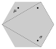
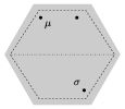
(a)		(b)

Figure 3.3. Although $\sigma$ and $\mu$ lie within the same cone, the choice of border vectors in (a) could mean the algorithm at first does not add a constraint to guarantee $\mathrm{lt}_{\sigma}\left(g_{\ell}\right)>\mathrm{lt}_{\mu}\left(g_{\ell}\right)$. If the narrowed cone splits later on, as in (b), and the algorithm moves into a subcone that does not contain $\sigma$, a subsequent choice of $\mu$ is possible, causing a change in the leading terms. We can try adding the previously-overlooked constraint, and continue if we find a feasible solution. The unlabeled dot could represent such a compromise ordering.

Thus, it would not add the constraint $\left(y_{1},\ldots,y_{n}\right)\cdot\left(\mathbf{t}-\mathbf{u}\right)>0$. A later choice of boundary vectors does recognize that $\mu\in C\left(\tau,\left\{g_{1},\ldots,g_{\ell+k}\right\}\right)$, and even selects $\mu$ as the ordering. We can see this in Figure 3.3(b). In this case, the leading term of $g_{\ell}$ changes from $t$ to $u$; the ordering has been changed, not refined!

Since the Gröbner basis property depends on the value of the leading terms, this endangers the algorithm’s correctness. Fortunately, it is easy to detect this situation; the algorithm simply monitors the leading terms.

It is not so easy to remedy the situation once we detect it. One approach is to add the relevant critical pairs to $P$, and erase any record of critical pairs computed with $g_{\ell}$, or discarded because of it. Any practical implementation of the dynamic algorithm would use criteria to discard useless critical pairs, such as those of Buchberger, but if the polynomials’ leading terms have changed, the criteria no longer apply. Recovering those pairs would require the addition of needless overhead.

A second approach avoids these quandaries: simply add the missing constraint to the system. This allows us to determine whether we were simply unlucky enough to choose $\sigma$ from a region of $C\left(\sigma,G\right)$ that lies outside $C\left(\mu,G\right)$, or whether really there is no way to choose both $\mathrm{lt}_{\sigma}\left(g_{\ell}\right)$ and $\mathrm{lt}_{\mu}\left(g_{\ell+k}\right)$ simultaneously. In the former case, the linear program will become infeasible, and we reject the choice of $\mu$; in the latter, we will be able to find $\tau\in C\left(\sigma,G\right)\cap C\left(\mu,G\right)$.

3.2.3. Implementation

Since the constraints of $\mathrm{lp}\left(\sigma,G\right)$ consist of integer polynomials, it is possible to find integer solutions for the boundary vectors; one simply rescales rational solutions once they are found. However, working with exact arithmetic can be quite slow, techniques of integer programming are very slow, and for our purposes, floating-point approximations are quite suitable. Besides, most linear solvers work with floating point numbers.

On the other hand, using floating point introduces a problem when comparing terms. The computer will sometimes infer $\omega\cdot\left(\mathbf{u}-\mathbf{t}\right)>0$ even though the exact representation would have $\omega\cdot\left(\mathbf{u}-\mathbf{t}\right)=0$. We can get around this by modifying the constraints of the linear program to $\omega\cdot\left(\mathbf{u}-\mathbf{t}\right)\geq\epsilon$ for some sufficiently large $\epsilon>0$. As we see in Figure 3.4,

Figure 3.4. Estimation of the corner points of $C\left(\sigma,G\right)$ by a perturbation of the inequalities. Each diagram shows a two-dimensional cross-section of a three-dimensional cone. The dashed lines on the connect actual boundary vectors. The diagram on the right connects boundary vectors of a perturbation of the system of linear inequalities. The perturbation is designed to give us interior points of the cone that are close to corner points.

the polygon no longer connects extrema, but points that approximate them. We might actually reject some potential leading terms $u$ on this account, but on the other hand, we never waste time with terms that are incompatible with the current ordering.

This modified linear program is in fact useful for computing feasible points to the original linear program as well.

Theorem 18.

Let $\epsilon>0$ and $J$ a finite subset of $\mathbb{N}$. The system of linear inequalities

$$\mathrm{lp}\left(\sigma,G\right)=\left\{\mathbf{a}^{\left(j\right)}\cdot\left(y_{1},\ldots,y_{n}\right)>0\right\}_{j\in J}\cup\left\{y_{j}>0\right\}_{j=1}^{n}$$

is feasible if and only if the linear program

$$\left\{\mathbf{a}^{\left(j\right)}\cdot\left(y_{1},\ldots,y_{n}\right)\geq\epsilon\right\}_{j\in J}\cup\left\{y_{j}\geq\epsilon\right\}_{j=1}^{n}$$

is also feasible.

Proof.

A solution to the linear program obviously solves the system of linear inequalities. Thus, suppose the system of linear inequalities has a solution $\sigma$. Let $\tau=b\sigma$, where $b\in\mathbb{N}$ is chosen large enough that $\tau_{k}\geq\epsilon$ for $k=1,\ldots,n$. For each $j\in J$, define

$$\gamma_{j}=\sum_{k=1}^{n}a_{k}^{\left(j\right)}\tau_{k},$$

then choose $c_{j}\geq 1$ such that $c_{j}\gamma_{j}\geq\epsilon$. Put $d=\max\left\{c_{j}\right\}_{j\in J}$. Let $\omega=d\tau$. We have $\omega_{k}\geq\tau_{k}\geq\epsilon$ for each $k=1,\ldots,n$, and

$$\mathbf{a}^{\left(j\right)}\cdot\omega=\sum_{k=1}^{n}a_{k}^{\left(j\right)}\omega_{k}=d\sum_{k=1}^{n}a_{k}^{\left(j\right)}\tau_{k}=d\gamma_{j}\geq c_{j}\gamma_{j}\geq\epsilon$$

for each $j\in J$. We have shown that $\omega$ is a solution to the linear program, which means that the linear program is also feasible. ∎

Based on Theorem 18, we take the following approach:

1. Replace each constraint $\mathbf{a}^{\left(j\right)}\cdot y>0$ of $\mathrm{lp}\left(\sigma,G\right)$ with $\mathbf{a}^{\left(j\right)}\cdot y\geq\epsilon$, add constraints $y_{k}\geq\epsilon$ for $k=1,\ldots,n$, and take as the objective function the minimization of $\sum y_{k}$. We denote this new linear program as $\mathrm{mlp}\left(\sigma,G\right)$.

2. Solve $\mathrm{mlp}\left(\sigma,G\right)$. This gives us a vector $\tau$ that can serve as a weighted ordering for the terms already computed.

3. Identify some $d\in\mathbb{R}$ such that $\mathrm{mlp}\left(\sigma,G\right)$ intersects the hyperplane $\sum y_{k}=d$, giving us a cross-section $K$ of the feasible region. This is trivial once we have a solution $\tau$ to $\mathrm{mlp}\left(\sigma,G\right)$, since we can put $d=1+\sum\tau_{k}$.

4. Compute an approximation to $\Omega$ by maximizing and minimizing each $y_{k}$ on $K$.

Algorithm compute_boundary_vectors (Figure 3.5)

 

algorithm compute_boundary_vectors

inputs:

• $L=\mathrm{mlp}\left(\sigma,G\right)$

• $\tau\in\mathbb{R}^{n}$ that solves $L$

outputs: $\Psi\subsetneq\mathbb{R}^{n}$, a set of vectors that approximates the boundary vectors of $\mathrm{mlp}\left(\sigma,G\right)$

do:

1. let $\Psi=\left\{\right\}$

2. let $d=1+\tau_{1}+\cdots+\tau_{n}$

3. let $L=L\cup\left\{y_{1}+\cdots+y_{n}=d\right\}$

4. for $k\in\left\{1,\ldots,n\right\}$

   1. add to $\Psi$ the solution $\omega$ of $L$ that maximizes $\omega_{k}$

   2. add to $\Psi$ the solution $\omega$ of $L$ that minimizes $\omega_{k}$

5. return $\Psi$

Figure 3.5. Algorithm to compute approximate boundary vectors to $C\left(G,\sigma\right)$

 

gives pseudocode to do this; it generates a set of boundary vectors $\Psi$ that approximates the set $\Omega$ of boundary vectors of $C\left(\sigma,G\right)$.

Once we have an approximation $\Psi$ to the boundary vectors $\Omega$, we use it to eliminate terms that cannot serve as leading terms within the current cone. Algorithm identify_clts_using_boundary_vectors (Figure 3.6),

 

algorithm identify_clts_using_boundary_vectors

inputs:

• $\sigma\in\mathcal{T}$, the current term ordering

• $t=\mathrm{lt}_{\sigma}\left(r\right)$, where $r\in R$

• $U=\mathrm{supp}\left(r\right)\backslash\left\{t\right\}$

• $\Psi\subsetneq\mathbb{R}^{n}$, approximations to the boundary vectors of $C\left(G,\sigma\right)$

outputs: $V$, where $v\in V$ iff $v=t$, or $v\in U$ and $\psi\left(\mathbf{v}-\mathbf{t}\right)>0$ for some $\psi\in\Psi$

do:

1. let $V=\left\{t\right\}$

2. for $u\in U$

   1. if $\psi\left(\mathbf{u}-\mathbf{t}\right)>0$ for some $\psi\in\Psi$

      1. add $u$ to $V$

3. return $V$

Figure 3.6. Eliminating terms using approximation to boundary vectors

 

accomplishes this by looking for $u\in\mathrm{supp}\left(r\right)\backslash\left\{\mathrm{lt}_{\sigma}\left(r\right)\right\}$ and $\psi\in\Psi$ such that $\psi\left(\mathbf{u}-\mathbf{t}\right)>0$. If it finds one, then $u$ is returned as a compatible leading term.

In Section 3.2.2, we pointed out that creating constraints only for the terms identified as potential leading terms by the use of boundary vectors can lead to an inconsistency with previously-chosen terms. For this reason, we not only try to solve the linear program, but invokes algorithm monitor_lts (Figure 3.7) to verify that previously-determined leading terms remain invariant.

 

algorithm monitor_lts

inputs

• $G$, the working basis

• $\sigma\in\mathcal{T}$, the old ordering

• $\tau\in\mathcal{T}$, a new ordering

• $L=\mathrm{mlp}\left(\tau,G\right)$

outputs

• (True, $\mu$) if there exists $\mu\in L$ refining $C\left(G,\sigma\right)$ and $\mathrm{lt}_{\mu}\left(g_{\textrm{last}}\right)=\mathrm{lt}_{\tau}\left(g_{\textrm{last}}\right)$, where $g_{\textrm{last}}$ is the newest element of $G$

• False otherwise

do:

1. let $\mu=\tau$

2. while there exists $g\in G$ such that $\mathrm{lt}_{\mu}\left(g\right)\neq\mathrm{lt}_{\sigma}\left(g\right)$

   1. for each $g\in G$ whose leading term changes

      1. let $t=\mathrm{lt}_{\sigma}\left(g\right)$, $u=\mathrm{lt}_{\mu}\left(g\right)$

      2. let $L=L\bigcup\left\{y\cdot\left(\mathbf{t}-\mathbf{u}\right)\right\}$

   2. if $L$ is infeasible return False
      else let $\mu$ be the solution to $L$

3. return (True, $\mu$)

Figure 3.7. Ensuring the terms remain invariant

 

If some leading terms would change, the algorithm obtains a compromise ordering whenever one exists.

Theorem 19.

Algorithm monitor_lts of Figure 3.7 terminates correctly.

Proof.

Termination is evident from the fact that $G$ is a finite list of polynomials, so the while loop can add only finitely many constraints to $L$. Correctness follows from the fact that the algorithm adds constraints to $\mathrm{mlp}\left(\tau,G\right)$ if and only if they correct changes of the leading term. Thus, it returns (True, $\mu$) if and only if it is possible to build a linear program $L$ whose solution $\mu$ lies in the non-empty set $C\left(\tau,G\right)\cap C\left(\sigma,G\right)$. ∎

It remains to put the pieces together.

 

algorithm dynamic_algorithm_with_geometric_criteria

inputs: $F\subseteq R$

outputs: $G\subseteq R$ and $\sigma\in\mathcal{T}$ such that $G$ is a Gröbner basis of $\left<F\right>$ with respect to $\sigma$

do:

1. Let $G=\left\{\right\}$, $P=\left\{\left(f,0\right):f\in F\right\}$, $\sigma\in\mathcal{T}$

2. Let $\textit{rejects}=\left\{\right\}$, $\Psi=\left\{e_{k}:k=1,\ldots,n\right\}$

3. while $P\neq\emptyset$

   1. Select $\left(p,q\right)\in P$ and remove it

   2. Let $r$ be a remainder of $\mathrm{spoly}\left(p,q\right)$ modulo $G$

   3. if $r\neq 0$

      1. Add $\left(g,r\right)$ to $P$ for each $g\in G$

      2. Add $r$ to $G$

      3. Select $\sigma\in\mathcal{T}$, using identify_clts_using_boundary_vectors to eliminate incompatible terms and monitor_lts to ensure consistency of $\tau$, storing failed linear programs in rejects

      4. Remove useless pairs from $P$

   4. Let $\Psi=$ compute_boundary_vectors($L$, $\mathrm{mlp}\left(\sigma,G\right)$)

4. return $G$, $\sigma$

Figure 3.8. A dynamic Buchberger algorithm that employs the Disjoint Cones and Boundary Vectors criteria

 

Theorem 20.

Algorithm dynamic_algorithm_with_geometric_criteria terminates correctly.

Proof.

The only substantive difference between this algorithm and the dynamic algorithm presented in [9] lies in line 3(c)iii. In the original, it reads∎

$\sigma:=\mathbf{RefineCurrentOrder}\left(f_{t+1},F,\sigma\right).$

Theorems 14, 18, and 19 are critical to correctness and termination of the modified algorithm, as they ensures refinement of the ordering, rather than change. In particular, the compatible leading terms identified by boundary vectors are indivisible by previous leading terms; since refinement preserves them, each new polynomial expands $\left<\mathrm{lt}\left(G\right)\right>$, and the Noetherian property of a polynomial ring applies.

4. Experimental results

The current study implementation, written in Cython for the Sage computer algebra system [28], is available at

www.math.usm.edu/perry/Research/dynamic_gb.pyx

It is structured primarily by the following functions:

• is the control program, which invokes the usual functions for a Buchberger algorithm (creation, pruning, and selection of critical pairs using the Gebauer-Möller algorithm and the sugar strategy, as well as computation and reduction of of $S$-polynomials), as well as the following functions necessary for a dynamic algorithm that uses the criteria of Disjoint Cones and Boundary Vectors:

  • which refines the ordering according to the Hilbert function heuristic, and invokes:

    • which applies the Boundary Vectors and Divisibility criteria;

    • which tries to extend the current linear program with constraints corresponding to the preferred leading term; it also applies the Disjoint Cones criterion, and invokes

      • which verifies that an ordering computed by feasible preserves the previous choices of leading terms;

  • which computes an approximation $\Psi$ to the boundary vectors $\Omega$.

The dynamic_gb function accepts the following options:

• static: boolean, True computes by the static method, while False (the default) computes by the dynamic method;

• strategy: one of ’sugar’, ’normal’ (the default), or ’mindeg’;

• weighted_sugar: boolean, True computes sugar according to ordering, while False (the default) computes sugar according to standard degree;

• use_boundary_vectors: boolean, default is True;

• use_disjoint_cones: boolean, default is True.

At the present time, we are interested in structural data rather than timings. To that end, experimental data must establish that the methods proposed satisfy the stated aim of reducing the size and number of linear programs constructed; in other words, the algorithm invokes the refiner only when it has high certainty that it is needed. Evidence for this would appear as the number of linear programs it does not construct, the number that it does, and the ratio of one to the other. We should also observe a relatively low number of failed linear programs.

Table 1 summarizes the performance of this implementation on several benchmarks. Its columns indicate:

• the name of a polynomial system tested;

• the number of linear programs (i.e., potential leading terms)

  • rejected using approximate boundary vectors,

  • rejected using disjoint cones,

  • solved while using the two new criteria,

  • solved while not using the new criteria, and

  • failed;

• the ratio of the linear programs solved using the new criteria to the number solved without them; and

• the number of constraints in the final program, both using the new criteria, and not using them.

Both to emphasize that the algorithm really is dynamic, and to compare with Caboara’s original results, Table 1 also compares:

• the size of the Gröbner basis generated by the dynamic algorithm, in terms of

  • the number of polynomials computed, and

  • the number of terms appearing in the polynomials of the basis;

• the size of the Gröbner basis generated by Singular’s std() function with the grevlex ordering, in the same terms.

	linear programs								final size
	rejected by…		solved				#constraints		dynamic		static
system	corners	disjoint	cor+dis	div only	$\frac{\mathrm{cor}+\mathrm{dis}}{\mathrm{div\,only}}$	failed	cor+dis	div only	#pols	#terms	#pols	#terms
Caboara 1	22	0	10	25	0.400	0	20	29	35	137	239	478
Caboara 2	19	0	20	10	2.222	10	26	17	21	42	553	1106
Caboara 4	64	0	10	20	0.500	2	26	30	9	20	13	23
Caboara 5	81	0	19	6	3.167	14	24	20	12	67	20	201
Caboara 6	15	0	7	8	0.875	1	16	16	7	15	7	15
Caboara 9	2	0	4	5	0.800	0	10	11	7	14	37	74
Cyclic-5	379	0	16	327	0.049	5	31	61	11	68	20	85
Cyclic-6	4,080	0	58	2800	0.021	43	56	250	20	129	45	199
Cyclic-7	134,158	12	145	*	*	108	147	*	63	1,049	209	1,134
Cyclic-5 hom.	128	0	17	259	0.066	7	33	60	11	98	38	197
Cyclic-6 hom.	1,460	0	25	1,233	0.020	16	39	303	33	476	99	580
Cyclic-7 hom.	62,706	0	38	*	*	20	105	*	222	5,181	443	3,395
Katsura-6	439	5	37	108	0.343	18	53	68	22	54	22	54
Katsura-7	1,808	3	43	379	0.113	33	109	205	49	104	41	105
Katsura-6 hom.	419	13	77	326	0.236	46	113	281	23	164	22	160
Katsura-7 hom.	1,920	24	114	1,375	0.083	63	234	731	46	352	41	354

*This system was terminated when using only the Divisibility Criterion, as the linear program had acquired more than 1000 constraints.

Table 1. Dynamic algorithm with sugar strategy, applying Divisibility Criterion after boundary vectors. Data for static algorithm included for comparison.

The systems “Caboara $i$” correspond to the example systems “Es $i$” from [9], some of which came from other sources; we do not repeat the details here. We verified by brute force that the final result was a Gröbner basis.

The reader readily sees that the optimizations introduced in this paper accomplish the stated goals. By itself, the method of boundary vectors eliminates the majority of incompatible leading terms. In the case of dense polynomial systems, it eliminates the vast majority. This means that far, far fewer linear programs are constructed, and those that are constructed have far fewer constraints than they would otherwise. While the number of inconsistent linear programs the algorithm attempted to solve (the “failed” column) may seem high in proportion to the number of programs it did solve (“solved”), this pales in comparison to how many it would have attempted without the use of boundary vectors; a glance at the “div only” column, which consists of monomials that were eliminated only by the Divisibility Criterion, should allay any such concerns.

Remark 21.

In two cases, the new criteria led the algorithm to compute more linear programs than if it had used the Divisibility Criterion alone. There are two reasons for this.

• One of the input systems (Caboara 2) consists exclusively of inhomogeneous binomials with many divisible terms. This setting favors the Divisibility Criterion. The other system (Caboara 5) also contains many divisible terms.

• For both systems, the sample set of boundary vectors wrongly eliminates compatible monomials that should be kept. While this suggests that the current strategy of selecting a sample set of boundary vectors leaves much to be desired, the dynamic algorithm computes a smaller basis than the static, and with fewer $S$-polynomials, even in these cases.

It should not startle the reader that the dynamic algorithm performs poorly on the homogeneous Katsura-$n$ systems, as Caboara had already reported this. All the same, boundary vectors and disjoint cones minimize the cost of the dynamic approach.

Many of our Gröbner bases have different sizes from those originally reported by Caboara. There are several likely causes:

• The original report had typographical errors. We have verified and corrected this in some cases, but some results continue to differ.

• The static ordering used here may order the variables differently from [9], which did not documented this detail. For example, Caboara reports a basis of only 318 polynomials for Caboara 2 when using the static algorithm with grevlex, but Sage (using Singular) finds 553.

• Several choices of leading term can have the same tentative Hilbert function, but one of the choices is in fact better than the others in the long run. The original implementation may have chosen differently from this one. In particular [9] gave a special treatment to the input polynomials, considering the possible leading term choices for all of them simultaneously, and not sequentially, one-by-one.

We conclude this section with a word on complexity. While the worst case time complexity of the simplex algorithm is exponential [22], on average it outperforms algorithms with polynomial time complexity. The computation of boundary vectors increases the number of invocations of simplex, but the large reduction in the number of monomials considered more than compensates for this. The space requirements are negligible, as we need only $2n$ boundary vectors at any one time, and the reduction in the number and size of the linear programs means the algorithm needs to remember only a very few disjoint cones. Considering how rarely the disjoint cones are useful, it might be worthwhile not to implement them at all, but we have not observed them to be a heavy burden at the current time.

5. Conclusion, future work

We set out to reduce the size and number of linear programs used by a dynamic algorithm to compute a Gröbner basis. Geometrical intuition led us to two methods that work effectively and efficiently. While the effect with the systems tested by Caboara was only moderate, and in some cases counterproductive, the story was different with the dense benchmark systems. In these cases, the number of refinements approached insignificance, and we continued to achieve good results. The final Gröbner basis was always of a size significantly smaller than grevlex; only a few refinements were required for the algorithm to be very effective.

A significant restraint imposed by many computer algebra systems is that a term ordering be defined by integers. As Sage is among these, this has required us to solve not merely linear programs, but pure integer programs. Integer programming is much more intensive than linear programming, and its effect was a real drag on some systems. There is no theoretical need for this; we plan to look for ways to eliminate this requirement, or at least mitigate it.

An obvious next step is to study various ambiguities in this approach. This includes traditional questions, such as the effect of the selection strategy of critical pairs, and also newer questions, such as generating the sample set of boundary vectors. We followed Caboara’s approach and used the sugar strategy. We expect the normal strategy [8] to be useful only rarely, while signature-based strategies [14][16], which eliminate useless pairs using information contained in the leading terms of a module representation, could combine with the dynamic algorithm to expand significantly the frontiers of the computation of Gröbner bases, and we are working towards such an approach.

Another optimization would be to use sparse matrix techniques to improve the efficiency of polynomial reduction in a Gröbner basis algorithm, a la F4. Combining this with a dynamic algorithm is comparable to allowing some column swaps in the Macaulay matrix, something that is ordinarily impossible in the middle of a Gröbner basis computation.

The authors would like to thank Nathann Cohen for some stimulating conversations, and his assistance with Sage’s linear programming facilities.

Appendix

Here we give additional information on one run of the inhomogeneous Cyclic-6 system. Computing a Gröbner basis for this ideal with the standard sugar strategy requires more $S$-polynomials than doing so for the ideal of the homogenized system; in our implementation, the number of $S$-polynomials is roughly equal to computing the basis using a static approach. (In general, the dynamic approach takes fewer $S$-polynomials, and the weighted sugar strategy is more efficient on this ideal.) Information on timings was obtained using Sage’s profiler:

• for the static run, we used

%prun B = dynamic_gb(F,static=True,strategy=’sugar’);

• for the dynamic run, we used

%prun B = dynamic_gb(F,static=False,strategy=’sugar’).

We obtained structural data by keeping statistics during a sample run of the program.

While Cython translates Python instructions to C code, then compiles the result, the resulting binary code relies on both the Python runtime and Python data structures; it just works with them from compiled code. Timings will reflect this; we include them merely to reassure the reader that this approach shows promise.

Our implementation of the dynamic algorithm uses 377 $S$-polynomials to compute a Gröbner basis of 20 polynomials, with 250 reductions to zero. At termination, $\mathit{rejects}$ contained 43 sets of constraints, which were never used to eliminate linear programs. As for timings, one execution of the current implementation took 25.45 seconds. The profiler identified the following functions as being the most expensive.

• Roughly half the time, 11.193 seconds, was spent reducing polynomials. (All timings of functions are cumulative: that is, time spent in this function and any other functions it invokes.) This is due to our having to implement manually a routine that would reduce polynomials and compute the resulting sugar. A lot of interpreted code is involved in this routine.

• Another third of the time, 8.581 seconds, was spent updating the critical pairs using the Gebauer-Möller update algorithm. Much of this time (3.248 seconds) was spent computing the lcm of critical pairs.

The majority of time (5/6) was spent on functions that are standard in the Buchberger algorithm! Ordinarily, we would not expect an implementation to spend that much time reducing polynomials and updating critical pairs; we are observing a penalty from the Python runtime and data structures. The size of this penalty naturally varies throughout the functions, but this gives the reader an idea of how large it can be.

Other expensive functions include:

• About 4.6 seconds were spent in choose_an_ordering. Much of this time (2.4 seconds) was spent sorting compatible leading terms according to the Hilbert heuristic.

• The 238 invocations of Sage’s hilbert_series and hilbert_polynomial took 1.5 seconds and 0.8 seconds, respectively. As Sage uses Singular for this, some of this penalty is due to compiled code, but Singular’s implementation of these functions is not state-of-the-art; techniques derived from [3] and [27] would compute the Hilbert polynomial incrementally and quickly.

• The 57 invocations of feasible consumed roughly 1.2 seconds. This includes solving both continuous and pure integer programs, and suffers the same penalty from interpreted code as other functions.

It is worth pointing out what is not present on this list:

• Roughly one quarter of a second was spent in monitor_lts.

• The boundary_vectors function took roughly one and a half tenths of a second (.016).

• Less than one tenth of a second was spent applying the Boundary Vectors Criterion in possible_lts.

If we remove the use of the Boundary Vector and Disjoint Cones criteria, the relative efficiency of feasible evaporates; the following invocation illustrates this vividly:

%prun B = dynamic_gb(F, strategy=’sugar’,

use_boundary_vectors=False,

use_disjoint_cones=False)

Not only is the Divisibility Criterion unable to stop us from solving 2,820 linear programs, but the programs themselves grow to a size of 247 constraints. At 41 seconds, feasible takes nearly twice as long as entire the computation when using the new criteria! This inability to eliminate useless terms effect cascades; hilbert_polynomial and hilbert_series are invoked 3,506 times, taking 12.6 and 28.6 seconds, respectively; choose_an_ordering jumps to 92.7 seconds, with 44 seconds wasted in applying the heuristic. By contrast, the timings for reduction of polynomials and sorting of critical pairs grow much, much less, to 20 seconds and 12.9 seconds, respectively. (The increase in reduction corresponds to an increase in the number of $S$-polynomials, probably due to a different choice of leading term at some point – recall that the approximation of boundary vectors excludes some choices.) The optimizations presented here really do remove one of the major bottlenecks of this method.

We conclude by noting that when we use the Disjoint Cones criterion alone, 1,297 invalid monomials are eliminated, but the number of constraints in the final linear program increases to 250; this compares to 4,080 monomials that Boundary Vectors alone eliminates, with 56 constraints in the final linear program.

References

- [1] Apel, J., Hemmecke, R.: Detecting unnecessary reductions in an involutive basis computation. Journal of Symbolic Computation 40(4–5), 1131–1149 (2005)
- [2] Bayer, D., Stillman, M.: Computation of Hilbert Functions. Journal of Symbolic Computation 14, 31–50 (1992)
- [3] Bigatti, A.M.: Computation of Hilbert-Poincaré Series. Journal of Pure and Applied Algebra 119(3), 237–253 (1997)
- [4] Bigatti, A.M., Caboara, M., Robbiano, L.: Computing inhomogeneous Gröbner bases. Journal of Symbolic Computation 46(5), 498–510 (2010). DOI 10.1016/j.jsc.2010.10.002
- [5] Brickenstein, M.: Slimgb: Gröbner bases with slim polynomials. Revista Matemática Complutense 23(2), 453–466 (2009)
- [6] Buchberger, B.: Ein Algorithmus zum Auffinden der Basiselemente des Restklassenringes nach einem nulldimensionalem Polynomideal (An Algorithm for Finding the Basis Elements in the Residue Class Ring Modulo a Zero Dimensional Polynomial Ideal). Ph.D. thesis, Mathematical Institute, University of Innsbruck, Austria (1965). English translation published in the Journal of Symbolic Computation (2006) 475–511
- [7] Buchberger, B.: A Criterion for Detecting Unnecessary Reductions in the Construction of Gröbner Bases. In: E.W. Ng (ed.) Proceedings of the EUROSAM 79 Symposium on Symbolic and Algebraic Manipulation, Marseille, June 26-28, 1979, Lecture Notes in Computer Science, vol. 72, pp. 3–21. Springer, Berlin - Heidelberg - New York (1979)
- [8] Buchberger, B.: Gröbner-Bases: An Algorithmic Method in Polynomial Ideal Theory. In: N.K. Bose (ed.) Multidimensional Systems Theory - Progress, Directions and Open Problems in Multidimensional Systems, pp. 184–232. Reidel Publishing Company, Dotrecht – Boston – Lancaster (1985)
- [9] Caboara, M.: A Dynamic Algorithm for Gröbner basis computation. In: ISSAC ’93, pp. 275–283. ACM Press (1993)
- [10] Caboara, M., Dominicis, G.D., Robbiano, L.: Multigraded hilbert functions and buchberger algorithm. In: E. Engeler, B. Caviness, Y. Lakshman (eds.) International Symposium of Symbolic and Algebraic Computation ISSAC ’96, pp. 72–78. ACM Press (1996)
- [11] Caboara, M., Kreuzer, M., Robbiano, L.: Minimal Sets of Critical Pairs. In: B. Cohen, X. Gao, N. Takayama (eds.) Proceedings of the First Congress of Mathematical Software, pp. 390–404. World Scientific (2002)
- [12] Calvert, J.E., Voxman, W.L.: Linear Programming. Harcourt Brace Jovanovich (1989)
- [13] Collart, S., Kalkbrenner, M., Mall, D.: Converting Bases with the Gröbner Walk. Journal of Symbolic Computation 24(3–4), 465–469 (1997)
- [14] Eder, C., Perry, J.: Signature-based algorithms to compute Gröbner bases. In: Proceedings of the 2011 International Symposium on Symbolic and Algebraic Computation (ISSAC ’11), pp. 99–106. ACM Press (2011). DOI 10.1145/1993886.1993906. Preprint available online at arxiv.org/abs/1101.3589
- [15] Faugère, J.C.: A New Efficient Algorithm for Computing Gröbner bases (F4). Journal of Pure and Applied Algebra 139(1–3), 61–88 (1999)
- [16] Faugère, J.C.: A new efficient algorithm for computing Gröbner bases without reduction to zero F5. In: International Symposium on Symbolic and Algebraic Computation Symposium - ISSAC 2002, Villeneuve d’Ascq, France, pp. 75–82 (2002). Revised version downloaded from fgbrs.lip6.fr/jcf/Publications/index.html
- [17] Faugère, J.C., Gianni, P., Lazard, D., Mora, T.: Efficient computation of zero-dimensional Gröbner bases by change of ordering. Journal of Symbolic Computation 16(4), 329–344 (1993)
- [18] Gebauer, R., Möller, H.: On an Installation of Buchberger’s Algorithm. Journal of Symbolic Computation 6, 275–286 (1988)
- [19] Giovini, A., Mora, T., Niesi, G., Robbiano, L., Traverso, C.: “One sugar cube, please” OR Selection strategies in the Buchberger algorithm. In: Proceedings of the 1991 International Symposium on Symbolic and Algebraic Computation, pp. 49–54. ACM Press (1991)
- [20] Golubitsky, O.: Converging term order sequences and the dynamic Buchberger algorithm (in preparation). Preprint received in private communication
- [21] Gritzmann, P., Sturmfels, B.: Minkowski Addition of Polytopes: Computational Complexity and Applications to Gröbner Bases. SIAM J. Disc. Math 6(2), 246–269 (1993)
- [22] Klee, V., Minty, G.: How good is the simplex algorithm? In: Inequalities III (Proceedings of the Third Symposium on Inequalities), pp. 159–175. Academic Press, New York-London (1972)
- [23] Kreuzer, M., Robbiano, L.: Computational Commutative Algebra 2. Springer-Verlag, Heidelberg (2005)
- [24] Mora, F., Möller, H.: New constructive methods in classical ideal theory. Journal of Algebra 100(1), 138–178 (1986)
- [25] Mora, T., Robbiano, L.: The Gröbner fan of an ideal. Journal of Symbolic Computation 6, 183–208 (1988)
- [26] Robbiano, L.: On the theory of graded structures. Journal of Symbolic Computation 2, 139–170 (1986)
- [27] Roune, B.H.: A Slice Algorithm for Corners and Hilbert-Poincaré Series of Monomial Ideals. In: Proceedings of the International Symposium on Symbolic and Algebraic Computation, pp. 115–122. ACM Press, New York (2010)
- [28] Stein, W.: Sage: Open Source Mathematical Software (Version 4.8). The Sage Group (2012). www.sagemath.org
- [29] Sultan, A.: Linear Programming: An Introduction with Applications (Second Edition). CreateSpace (2011)
- [30] Tran, Q.N.: Ideal-Specified Term Orders for Elimination and Applications in Implicitization. In: Proceedings of the Tenth International Conference on Applications of Computer Algebra, pp. 15–24. International Scientific Committee for Applications of Computer Algebra, Beaumont, TX (2005). Selected papers to appear in a forthcoming issue of the Journal of Symbolic Computation
- [31] Tran, Q.N.: A new class of term orders for elimination. Journal of Symbolic Computation 42(5), 533–548 (2007)
- [32] Traverso, C.: Hilbert functions and the buchberger algorithm. Journal of Symbolic Computation 22(4), 355–376 (1996)
- [33] Yan, T.: The Geobucket Data Structure for Polynomials. Journal of Symbolic Computation 25, 285–293 (1998)
- [34] Zharkov, A.Y., A. Blinkov, Y.: Involution Approach to Investigating Polynomial Systems. Mathematics and Computers in Simulation 42(4–6), 323–332 (1996). DOI 10.1016/S0378-4754(96)00006-7