Counting statistics for genetic switches based on effective interaction approximation

Abstract

Applicability of counting statistics for a system with an infinite number of states is investigated. The counting statistics has been studied a lot for a system with a finite number of states. While it is possible to use the scheme in order to count specific transitions in a system with an infinite number of states in principle, we have non-closed equations in general. A simple genetic switch can be described by a master equation with an infinite number of states, and we use the counting statistics in order to count the number of transitions from inactive to active states in the gene. To avoid to have the non-closed equations, an effective interaction approximation is employed. As a result, it is shown that the switching problem can be treated as a simple two-state model approximately, which immediately indicates that the switching obeys non-Poisson statistics.

I Introduction

Counting statistics is a scheme to calculate all statistics related to specific transitions in a stochastic system. In the counting statistics, a master equation with discrete states is used to derive time-evolution equations for generating functions related to the specific transitions. The scheme has been used to investigate Förster resonance energy transfer, and many successful results have been obtained Gopich2003 ; Gopich2005 ; Gopich2006 . Although the scheme is basically formulated for a system with a finite number of states, it is possible to use the scheme to investigate a system with an infinite number of states. However, as exemplified later, we have non-closed equations in general, so that it would be needed to develop approximation schemes suitable for specific systems. As a first step, it is important to check whether an approximation scheme for the counting statistics is available for the system with an infinite number of states or not.

In the present paper, we focus on dynamics in genetic switches. It has been shown that stochastic behavior plays an important role in gene regulatory systems Elowitz2002 ; Rao2002 ; Kaern2005 , and there are many studies for the stochasticity in the gene regulatory systems from experimental points of view (e.g., see Gardner2000 ; Okano2008 ) and theoretical ones (e.g., see Hasty2000 ; Sasai2003 ; Hornos2005 ; Xu2006 ; Schultz2007 ; Shahrezaei2008 ; Walczak2009 ; Venegas-Ortiz2011 ). Not only studies by numerical simulations, but also those by analytical calculations have been performed. Some analytical expressions for the static properties, i.e., stationary distributions for the number of proteins or mRNAs, have already been obtained. In addition, in order to investigate the role of the stochasticity in genetic switches, dynamical properties, i.e., switching behavior between active and inactive gene states, have also been studied. Basically, such dynamical properties have been investigated by numerical simulations (e.g., see Feng2011 ); only for a simple system, analytical expressions for the first-passage time distribution have been obtained Visco2009 . The genetic switch is described by a master equation with an infinite number of states. Hence, if we can use the scheme of the counting statistics in order to investigate the dynamical properties in the genetic switches, it will be helpful to obtain deeper understanding and intuitive pictures for the genetic switches.

The aim of the present paper is to seek the applicability of the counting statistics in order to investigate the dynamical property in the genetic switches. It immediately becomes clear that a straightforward application of the counting statistics derives intractable non-closed equations. In order to obtain simple closed forms, we here employ an effective interaction approximation Ohkubo2011 . As a result, we will show that the switching problem can be treated as a simple two-state model approximately. This result immediately gives us intuitive understanding for the switching behavior and the non-Poissonian property.

The present paper is constructed as follows. In Sec. II, we give a brief explanation of a stochastic model for the genetic switch. In Sec. III, the counting statistics is employed in order to count the number of transitions in the genetic switch, and, as a result, a simple two-state model is derived approximately. The derived approximated results are compared with those of Monte Carlo simulations in Sec. IV. Section V gives concluding remarks.

II Model

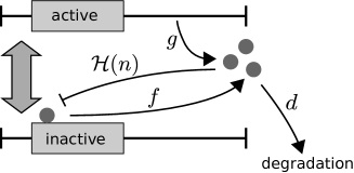
Figure 1: A schematic illustration of the self-regulating gene with repressed binding interaction. When the regulatory proteins are combining the gene, the gene is repressed and there is no production of proteins. If the regulatory proteins are released from the gene, the gene becomes active and it can produce the proteins. We consider the transition between the active and inactive states as a switch.

A gene regulatory system consists of many components, such as genes, RNAs, and proteins. Here, a simplified model is used; mRNAs are neglected for simplicity, and an activated gene assumes to directly increase the number of proteins. In addition, in the simplified model, a repressed gene cannot produce any proteins. The above model has been used to investigate the switching behavior in previous works, and, for example, see Schultz2007 for details of the model.

We summarize the model studied in the present paper in Fig. 1. The binding interaction is assumed to be a repressed one, and the gene is activated only when the regulatory proteins are not binding the gene. The proteins are produced from the gene in the active state with rate $g$, and proteins are degraded spontaneously with rate $d$. The regulatory proteins bind the gene with a rate function $\mathcal{H}(n)$, where $n$ is the number of free proteins. For example, $\mathcal{H}(n)=hn$ for a monomer interaction case, and $\mathcal{H}(n)=hn(n-1)/2$ for a dimer interaction case, where $h$ is a rate constant for the binding. $f$ is a rate constant with which the regulatory proteins are released from the repressor site of the gene.

We here give short comments for the model from the viewpoint of experiments. Using this simplified model, we can discuss the connection among the model parameters, the number of proteins, and the switching behaviors. While the number of proteins $n$ can be observed or estimated experimentally, as far as we know, there has not been an experimental technique to observe the attachment and detachment of the regulatory proteins directly. We hope that developments of single-molecule observations in future would enable us to give information about the switching dynamics.

III Counting statistics for the number of transitions

III.1 Master equation for the number of proteins

Analytical treatments for the self-regulating gene system have been developed, and an exact solution is known for the monomer interaction case, i.e., $\mathcal{H}(n)=hn$ Hornos2005 ; Visco2009 . In order to simplify the analytical treatments, an additional assumption has been used in some previous works Schultz2007 ; Ohkubo2011 ; i.e., some of proteins are assumed to be inert when the gene state is active. The inert proteins cannot repress the gene, and it is not degraded. For the monomer interaction case, there is only one inert protein; the number of inert protein for the dimer interaction case is two, and so on. Note that the assumption of the inert proteins does not have physical meanings; this only simplify the analytical treatments (for details, see Schultz2007 ). However, it has been shown that this assumption has little influence of the gene system, and then we employ the assumption in the present paper.

Let $\alpha_{n}$ and $\beta_{n}$ be states in which there are $n$ free proteins for the active and inactive states, respectively. The probabilities for $\alpha_{n}$ and $\beta_{n}$ at time $t$ satisfy the following master equations;

$$\frac{dP(\alpha_{n},t)}{dt}= g[P(\alpha_{n-1},t)-P(\alpha_{n},t)]$$

$$+d[(n+1)P(\alpha_{n+1},t)-nP(\alpha_{n},t)]$$

$$-hnP(\alpha_{n},t)+fP(\beta_{n},t),$$ (1)

$$\frac{dP(\beta_{n},t)}{dt}= d[(n+1)P(\beta_{n+1},t)-nP(\beta_{n},t)]$$

$$+hnP(\alpha_{n},t)-fP(\beta_{n},t),$$ (2)

where $P(\alpha_{n},t)$ and $P(\beta_{n},t)$ are probabilities for $n$ free proteins for the active and inactive states, respectively.

As stated in Sec. I, the exact solutions for stationary distributions of the number of proteins have been derived, and those are expressed using the Kummer confluent hypergeometric functions. For details, see Hornos2005 ; Schultz2007 .

III.2 Counting statistics

Using the concept of the counting statistics Gopich2003 ; Gopich2005 ; Gopich2006 , it is possible to investigate dynamical properties, i.e., all statistics for the switching behavior between the active and inactive states. In the present paper, as an example, we calculate the number of transitions from the inactive state to the active state. The generating functions for the transitions are immediately obtained from the master equations (1) and (2). A brief explanation of the counting statistics is given in the Appendix, and we here give consequences of the counting statistics.

A probability, with which there are $k$ transitions from the inactive state to the active state during time $t$, is denoted by $P(k|t)$. The generating function for $P(k|t)$ is defined as

$$F(\lambda,t)=\sum_{k=0}^{\infty}P(k|t)\lambda^{k},$$ (3)

where $\lambda$ is a counting variable. The generating function gives all information related to “inactive $\to$ active” transitions. According to the scheme of counting statistics, we split $F(\lambda,t)$ into restricted generating functions $\{\phi(\alpha_{n},\lambda,t)\}$ and $\{\phi(\beta_{n},\lambda,t)\}$, where $\phi(\alpha_{n},\lambda,t)$ and $\phi(\beta_{n},\lambda,t)$ are the generating functions for the system in states $\alpha_{n}$ and $\beta_{n}$ at time $t$, respectively. Using the scheme of the counting statistics, we obtain the following time-evolution equations for the restricted generating functions $\{\phi(\alpha_{n},\lambda,t)\}$ and $\{\phi(\beta_{n},\lambda,t)\}$:

$$\frac{d\phi(\alpha_{n},\lambda,t)}{dt}= g[\phi(\alpha_{n-1},\lambda,t)-\phi(\alpha_{n},\lambda,t)]$$

$$+d[(n+1)\phi(\alpha_{n+1},\lambda,t)-n\phi(\alpha_{n},\lambda,t)]$$

$$-hn\phi(\alpha_{n},\lambda,t)+\lambda f\phi(\beta_{n},\lambda,t),$$ (4)

$$\frac{d\phi(\beta_{n},\lambda,t)}{dt}= d[(n+1)\phi(\beta_{n+1},\lambda,t)-n\phi(\beta_{n},\lambda,t)]$$

$$+hn\phi(\alpha_{n},\lambda,t)-f\phi(\beta_{n},\lambda,t).$$ (5)

Although Eqs. (4) and (5) are similar to Eqs. (1) and (2), note that the final term in the right hand side of Eq. (4) has a factor $\lambda$. The factor $\lambda$ is introduced in order to count the number of transitions, and we can count the number of transitions related to this term (for details, see Appendix). Using the above restricted generating functions, the generating function $F(\lambda,t)$ is calculated as

$$F(\lambda,t)=\sum_{n=0}^{\infty}\left\{\phi(\alpha_{n},\lambda,t)+\phi(\beta_{n},\lambda,t)\right\}.$$ (6)

Next, we introduce the following generating functions for $\phi(\alpha_{n},\lambda,t)$ and $\phi(\beta_{n},\lambda,t)$:

$$\alpha(\lambda,z,t)\equiv\sum_{n=0}^{\infty}\phi(\alpha_{n},\lambda,t)z^{n},$$ (7)

$$\beta(\lambda,z,t)\equiv\sum_{n=0}^{\infty}\phi(\beta_{n},\lambda,t)z^{n}.$$ (8)

It is straightforward to derive the time-evolution equations for the new generating functions $\alpha(\lambda,z,t)$ and $\beta(\lambda,z,t)$ from Eqs. (4) and  (5);

$$\frac{d\alpha(\lambda,z,t)}{dt}= (z-1)\left[g\alpha(\lambda,z,t)-d\frac{\partial\alpha(\lambda,z,t)}{\partial z}\right]$$

$$-hz\frac{\partial\alpha(\lambda,z,t)}{\partial z}+\lambda f\beta(\lambda,z,t),$$ (9)

$$\frac{d\beta(\lambda,z,t)}{dt}= -(z-1)d\frac{\partial\beta(\lambda,z,t)}{\partial z}$$

$$+hz\frac{\partial\alpha(\lambda,z,t)}{\partial z}-f\beta(\lambda,z,t).$$ (10)

Using the generating function $\alpha(\lambda,z,t)$ and $\beta(\lambda,z,t)$, the generating function $F(\lambda,t)$ is given by

$$F(\lambda,t)=\alpha(\lambda,z=1,t)+\beta(\lambda,z=1,t),$$ (11)

and therefore it is enough to solve the following time-evolution equations in order to calculate the generating function $F(\lambda,t)$:

$$\frac{d\alpha(\lambda,t)}{dt}= -h\left.\frac{\partial\alpha(\lambda,z,t)}{\partial z}\right|_{z=1}+\lambda f\beta(\lambda,t),$$ (12)

$$\frac{d\beta(\lambda,t)}{dt}= h\left.\frac{\partial\alpha(\lambda,z,t)}{\partial z}\right|_{z=1}-f\beta(\lambda,t),$$ (13)

where we define $\alpha(\lambda,t)\equiv\alpha(\lambda,z=1,t)$ and $\beta(\lambda,t)\equiv\beta(\lambda,z=1,t)$.

Note that Eqs. (12) and (13) contain the derivative of $\alpha(\lambda,z,t)$ with respect to $z$. Hence, the equations are not closed. If these terms are expressed simply using $\alpha(\lambda,t)$, we will have simultaneous differential equations written only by the generating functions $\alpha(\lambda,t)$ and $\beta(\lambda,t)$; i.e., we have closed equations and hence the obtained equations may be solved analytically. In the following analysis, an effective interaction approximation is employed, and we will show that the above statistics can be approximated by a simple two-state model.

III.3 Approximation for the interaction

In the effective interaction approximation, the interaction function $\mathcal{H}(n)$ is replaced as a constant value. As shown in Ohkubo2011 , the dependence of $\mathcal{H}(n)$ on $n$ makes it difficult to obtain analytical results, and it has been shown that the approximation gives qualitatively good results.

Replacing the interaction function $\mathcal{H}(n)$ as

$$\mathcal{H}(n)=\tilde{h},$$ (14)

where $\tilde{h}$ is a constant, we obtain the following equations instead of Eqs. (12) and (13):

$$\frac{d\alpha(\lambda,t)}{dt}= -\tilde{h}\alpha(\lambda,t)+\lambda f\beta(\lambda,t),$$ (15)

$$\frac{d\beta(\lambda,t)}{dt}= \tilde{h}\alpha(\lambda,t)-f\beta(\lambda,t).$$ (16)

Note that Eqs. (15) and (16) are written only by $\alpha(\lambda,t)$ and $\beta(\lambda,t)$. It means that the switching problem can be approximated as a simple two-state model if the effective interaction $\tilde{h}$ is chosen adequately.

We here briefly explain the choice of the effective interaction $\tilde{h}$ using a simple example, i.e., the monomer binding interaction case. For the monomer binding interaction, the interaction function is calculated as follows Ohkubo2011 . In this case, the interaction function is $hn$. In order to obtain the effective interaction $\tilde{h}$, the number of proteins $n$ is replaced as the average number of proteins, i.e.,

$$\tilde{h}=h\langle n\rangle_{\alpha},$$ (17)

where $\langle n\rangle_{\alpha}$ is the expectation of the number of free regulatory proteins under a condition that the gene is in the active state (conditional expectation).

The conditional expectation can be calculated from the stationary distribution of the number of proteins. Note that the generating functions $\alpha(\lambda,z,t)$ and $\beta(\lambda,z,t)$ are reduced to generating functions for the stationary distribution of the number of proteins when $\lambda=1$. Hence, as shown in Ohkubo2011 , they are written as follows.

$$\alpha(z)\equiv \lim_{t\to\infty}\alpha(\lambda=1,z,t)=AF[a,b,N(z-1)],$$ (18)

$$\beta(z)\equiv \lim_{t\to\infty}\beta(\lambda=1,z,t)$$

$$= \left(1+\frac{\tilde{h}}{f}\right)AF[a-1,b-1,N(z-1)]-\alpha(z)$$ (19)

where $A=f/(f+\tilde{h})$ and

$$N=\frac{g}{d},\quad a=1+\frac{f}{d},\quad b=1+\frac{f+\tilde{h}}{d}.$$

$F(p,q,r)$ is the Kummer confluent hypergeometric function,

$$F(p,q,r)\equiv\sum_{n=0}^{\infty}\frac{(p)_{n}}{(q)_{n}}\frac{r^{n}}{n!},$$ (20)

where $(p)_{n}=p(p+1)(p+2)\cdots(p+n-1)$. We, therefore, obtain

$$\langle n\rangle_{\alpha}\equiv\frac{1}{\alpha(1)}\left.\frac{\partial}{\partial z}\alpha(z)\right|_{z=1}=\frac{g(d+f)}{d(d+f+\tilde{h})}.$$ (21)

By inserting Eq. (21) into Eq. (17), the following self-consistent equation is derived:

$$\tilde{h}=h\frac{g(d+f)}{d(d+f+\tilde{h})}.$$ (22)

Solving Eq. (22), we obtain

$$\tilde{h}=\frac{-(d^{2}+fd)+\sqrt{(d^{2}+fd)^{2}+3hgd(d+f)}}{2d}.$$ (23)

We finally comment on a solution of the simple two-state model (Eqs. (15) and (16)). The simple two-state model can be solved exactly Gopich2003 ; Gopich2006 , and the probability distribution $P(k|t)$ for the number of “inactive $\to$ active” transitions during time $t$ is explicitly written as follows:

$$P(k|t)= \left(\frac{(1-\gamma^{2})T}{2\gamma}\right)^{k}\frac{e^{-T}}{k!\sqrt{8\gamma T/\pi}}$$

$$\times\left\{2\gamma(k+T)I_{k-1/2}(\gamma T)+(1+\gamma^{2})TI_{k+1/2}(\gamma T)\right\},$$ (24)

where $T=(f+\tilde{h})t/2$, $\gamma^{2}=1-4f\beta(1)/(f+\tilde{h})$, and $I_{n}(z)$ are modified Bessel functions of the first kind. This expression (24) immediately gives us the non-Poissonian picture of the phenomenon.

IV Numerical results

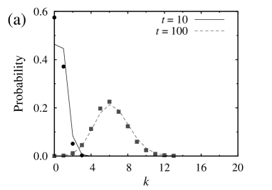
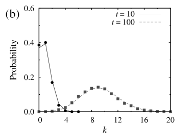
Figure 2: Probability distributions for the number of “inactive $\to$ active” transitions. (a) Monomer binding interaction case. (b) Dimer binding interaction case. In each figure, filled circles and filled boxes are Monte Carlo results for time $t=10$ and $t=100$, respectively. Solid and dashed lines corresponds to approximated analytical results of Eq. (24) for time $t=10$ and $t=100$, respectively.

In order to check the validity of the analytical treatments and the approximations, we here compare the analytical results with those of Monte Carlo simulations. The original genetic switch explained in Sec. II was simulated using a standard Gillespie algorithm Gillespie1977 . The parameters used in the simulation are as follows: $d=1,\quad g=50.0,\quad h=0.004,\quad f=0.1$. Note that these parameters were selected as one of the typical values used in the previous works Schultz2007 ; Ohkubo2011 .

Firstly, we consider the monomer binding interaction case. According to the discussions in Sec. 3.3, the value of the effective interaction $\tilde{h}$ is calculated as $\tilde{h}=0.173$. Figure 2(a) shows the results of the analytical calculations (Eq. (24)) and those of the Monte Carlo simulations. Although there are quantitative differences, the results shows that the approximated two-state model captures the essential features of the phenomenon.

Next, we consider a dimer binding interaction case, i.e., $\mathcal{H}(n)=hn(n-1)/2$. In this case, the effective interaction is calculated as follows:

$$\tilde{h}=h\frac{\langle n(n-1)\rangle_{\alpha}}{2}.$$ (25)

As shown in Ohkubo2011 , the effective interaction $\tilde{h}$ is obtained by solving the following self-consistent equation:

$$\tilde{h}=\frac{h}{2}\frac{1}{\alpha(1)}\left.\frac{\partial^{2}}{\partial z^{2}}\alpha(z)\right|_{z=0}.$$ (26)

We here numerically solved the self-consistent equation (Eq. (26)), and the calculated value of the effective interaction is $\tilde{h}=1.358$. Using the calculated value, we depict the analytical results and the corresponding Monte Carlo results in Fig. 2(b). From the comparison, we confirmed that the approximated two-state model is available even in the dimer binding interaction case. Although results are not shown, we performed numerical simulations for other some parameters, and checked the validity of the analytical treatments. For example, even for parameter regions in which the probability distribution of the number of proteins has bistability, the approximation scheme works well.

V Conclusions

In the present paper, we studied an analytical scheme to extract information related to the dynamical behavior in genetic switches. Using an effective interaction approximation, a simple two-state model is obtained, and we confirmed that the two-state model captures the features of the phenomenon. Note that in the analytical treatments, we did not neglect the stochastic properties of the system (except for the effective interaction approximation); i.e., we can calculate all statistics for transitions approximately, including higher order moments. It could be possible to apply the above effective expression for the transitions between the active and inactive states to more complicated gene regulatory networks without loss of the stochasticity; this would give us deeper understanding for the switching behavior of the gene regulatory systems including static, dynamical, and stochastic behaviors. In addition, the idea of the effective interaction may be similar to the mean-field approximation in statistical physics; the interaction is replaced with the average. It may be possible to develop higher-order approximations using the analogy with the conventional approximation schemes in statistical physics; this is an important future work.

We discussed properties only in the stationary states, because the effective interaction approximation has been applied only for the stationary states at the moment; the average number of proteins (or higher moments) should be estimated adequately, and it was calculated by using the analytical solutions for the stationary distributions of the number of proteins. Recently, exact time-dependent solutions for a self-regulating gene have been derived Ramos2011 . Hence, it may be possible to extend the effective interaction approximation to non-stationary states. If so, the effective interaction $\tilde{h}$ would be time-dependent, and, at least numerically, it is possible to calculate various moments for the counting statistics for time-dependent systems Ohkubo2010 . We expect that the simple description developed in the present paper is available for various cases, such as complicated regulatory systems and time-dependent systems, and that the description gives new insights for the regulation mechanisms and stochastic behaviors.

Appendix A Generating function for counting statistics

Here, we give a brief explanation for the counting statistics for readers’ convenience (For details, see Gopich2003 ; Gopich2005 ; Gopich2006 .) In the framework of counting statistics, the quantity of interest is the number of target transitions. It is needed to set multiple target transitions in the genetic switches, and the genetic switches have two states, i.e., active and inactive states. In the following explanations, a simple setting, in which there is only one transition matrix and only one target transition, will be discussed because it is straightforward to apply the following simple discussions to the genetic switches.

Let $\{K_{nm}\}$ be a transition matrix. We here derive the generating function for counting the number of events of a specific target transition $i_{\mathrm{A}}\to j_{\mathrm{A}}$. Denote the probability, with which the system starts from state $m$ and finishes in state $n$ with $k$ transitions from $i_{\mathrm{A}}$ to $j_{\mathrm{A}}$ during time $t$, as $P_{nm}(k|t)$. In order to calculate the probability $P_{nm}(k|t)$, we here define a probability $G_{kl}^{\prime}(t)$ with which the system evolves from state $l$ to state $k$, provided no $i_{\mathrm{A}}\to j_{\mathrm{A}}$ transitions occur during time $t$. By using the probability $G_{kl}^{\prime}(t)$, the probability $P_{nm}(k|t)$ is calculated as

$$P_{nm}(k|t)=$$

$$\quad G_{nj_{\mathrm{A}}}^{\prime}(t)\ast\underbrace{K_{j_{\mathrm{A}}i_{\mathrm{A}}}(t)G_{i_{\mathrm{A}}j_{\mathrm{A}}}^{\prime}(t)\ast\cdots\ast K_{j_{\mathrm{A}}i_{\mathrm{A}}}(t)G_{i_{\mathrm{A}}j_{\mathrm{A}}}^{\prime}(t)}_{k-1}$$

$$\quad\ast K_{j_{\mathrm{A}}i_{\mathrm{A}}}(t)G_{i_{\mathrm{A}}m}^{\prime}(t),$$ (27)

where $g_{1}(t)\ast g_{2}(t)\equiv\int_{0}^{t}g_{1}(t-t^{\prime})g_{2}(t^{\prime})dt^{\prime}$ denotes the convolution. This formulation means that an occurrence of the target transition $i_{\mathrm{A}}\to j_{\mathrm{A}}$ is sandwiched in between situations with no occurrence of the target transition, and it is repeated $k$ times.

Next, we construct the generating function $\tilde{\phi}_{nm}(\chi,t)$ of the probability $P_{nm}(k|t)$:

$$\tilde{\phi}_{nm}(\chi,t)=\sum_{k=0}^{\infty}\lambda^{k}P_{nm}(k|t).$$ (28)

That is, the generating function $\tilde{\phi}_{nm}(\lambda,t)$ gives the statistics of the number of transition $i_{\mathrm{A}}\to j_{\mathrm{A}}$ during time $t$ under the condition that the system starts from state $m$ and ends in state $n$. The generating function $\tilde{\phi}_{nm}(\lambda,t)$ satisfies the following integral equation

$$\tilde{\phi}_{nm}(\lambda,t)$$

$$=G_{nm}^{\prime}(t)+\int_{0}^{t}G_{nj_{\mathrm{A}}}^{\prime}(t-t^{\prime})\lambda K_{j_{\mathrm{A}}i_{\mathrm{A}}}(t^{\prime})\tilde{\phi}_{i_{\mathrm{A}}m}(\lambda,t^{\prime})dt^{\prime},$$ (29)

and obeys the following time-evolution equation

$$\frac{d}{dt}\tilde{\phi}_{nm}(\lambda,t)$$

$$\quad=\sum_{i}K_{ni}(t)G_{im}^{\prime}(t)-\delta_{n,j_{\mathrm{A}}}K_{j_{\mathrm{A}}i_{\mathrm{A}}}(t)G_{i_{\mathrm{A}}m}^{\prime}(t)$$

$$\qquad+\lambda G_{nj_{\mathrm{A}}}^{\prime}(0)K_{j_{\mathrm{A}}i_{\mathrm{A}}}(t)\tilde{\phi}_{i_{\mathrm{A}}m}(t)$$

$$\qquad+\int_{0}^{t}\left(\frac{d}{dt}G_{nj_{\mathrm{A}}}^{\prime}(t-t^{\prime})\right)\lambda K_{j_{\mathrm{A}}i_{\mathrm{A}}}(t^{\prime})\tilde{\phi}_{i_{\mathrm{A}}m}(t^{\prime})dt^{\prime}$$

$$\quad=\sum_{i}K_{ni}(t)\tilde{\phi}_{im}(\lambda,t)-\delta_{n,j_{\mathrm{A}}}(1-\lambda)K_{j_{\mathrm{A}}i_{\mathrm{A}}}(t)\tilde{\phi}_{i_{\mathrm{A}}m}(\lambda,t),$$ (30)

where $\tilde{\phi}_{nm}(\lambda,0)=\delta_{n,m}$. In order to show (30), we used the following two facts. Firstly, the probability of no target transitions, $G_{nm}^{\prime}(t)$, obeys

$$\frac{d}{dt}G_{nm}^{\prime}(t)=\sum_{i}K_{ni}(t)G_{im}^{\prime}(t)-\delta_{n,j_{\mathrm{A}}}K_{j_{\mathrm{A}}i_{\mathrm{A}}}(t)G_{i_{\mathrm{A}}m}^{\prime}(t),$$ (31)

where $G_{nm}^{\prime}(0)=\delta_{n,m}$. Secondly, the derivative of the convolution is given by

$$\frac{d}{dt}\int_{0}^{t}g_{1}(t-t^{\prime})g_{2}(t^{\prime})dt^{\prime}$$

$$=g_{1}(0)g_{2}(t)+\int_{0}^{t}\left(\frac{d}{dt}g_{1}(t-t^{\prime})\right)g_{2}(t^{\prime})dt^{\prime}.$$ (32)

Using the generating function $\tilde{\phi}_{nm}(\lambda,t)$, we construct restricted generating functions $\{\phi_{n}(\lambda,t)\}$ as follows:

$$\phi_{n}(\lambda,t)=\sum_{m}\tilde{\phi}_{nm}(\lambda,t)p_{m}(0),$$ (33)

where $p_{m}(0)$ is a probability distribution at initial time $t=0$. From (30) and (33), the restricted generating function satisfies

$$\frac{d}{dt}\phi_{n}(\lambda,t)$$

$$=\sum_{i}K_{ni}(t)\phi_{i}(\lambda,t)-\delta_{n,j_{\mathrm{A}}}(1-\lambda)K_{j_{\mathrm{A}}i_{\mathrm{A}}}(t)\phi_{i_{\mathrm{A}}}(\lambda,t),$$ (34)

and these equations should be solved with initial conditions $\phi_{n}(\lambda,0)=\sum_{m}\tilde{\phi}_{nm}(\lambda,0)p_{m}(0)=p_{n}(0)$. The summation of $\{\phi_{n}(\lambda,t)\}$ for $n$ gives the objective generating function for counting the number of events of the specific target transition.

References

- (1) I.V. Gopich and A. Szabo, J. Chem. Phys. 118, 454 (2003).
- (2) I.V. Gopich and A. Szabo, J. Chem. Phys. 122, 014707 (2005).
- (3) I.V. Gopich and A. Szabo, J. Chem. Phys. 124, 154712 (2006).
- (4) M.B. Elowitz, A.J. Levine, E.D. Siggia, and P.S. Swain, Science 297, 1183 (2002).
- (5) C.V. Rao, D.M. Wolf, and A.P. Arkin, Nature 420, 231 (2002).
- (6) M. Kærn, T.C. Elston, W.J. Blake, and J.J Collins, Nature Rev. Genetics 6, 451 (2005).
- (7) T.S. Gardner, C.R. Cantor, and J.J. Collins, Nature 403, 342 (2000).
- (8) H. Okano, T.J. Kobayashi, H. Tozaki, and H. Kimura, Biophys. J. 95, 1063 (2008).
- (9) J. Hasty, J. Pradines, M. Dolnik, and J.J Collins, Proc. Natl. Acad. Sci U.S.A 97, 2075 (2000).
- (10) M. Sasai and P.G. Wolynes, Proc. Natl. Acad. Sci U.S.A 100, 2374 (2003).
- (11) J.E.M. Hornos, D. Schultz, G.C.P. Innocentini, J. Wang, A.M. Walczak, J.N. Onuchic, and P.G. Wolynes, Phys. Rev. E 72, 051907 (2005).
- (12) B.-L. Xu and Y. Tao, J. Theor. Biol. 243, 214 (2006).
- (13) D. Schultz, J.N. Onuchic, and P.G. Wolynes, J. Chem. Phys. 126, 245102 (2007).
- (14) V. Shahrezaei and P.S. Swain, Proc. Natl. Acad. Sci U.S.A 105, 17256 (2008).
- (15) A.M. Walczak and P.G. Wolynes, Biophy. J. 96, 4525 (2009).
- (16) J. Venegas-Ortiz and M.R. Evans, J. Phys. A: Math. Theor. 44, 355001 (2011).
- (17) H. Feng, B. Han, and J. Wang, J. Phys. Chem. B 115, 1254 (2011).
- (18) P. Visco, R.J. Allen, and M.R. Evans, Phys. Rev. E 79, 031923 (2009).
- (19) J. Ohkubo, Phys. Rev. E 83, 041915 (2011).
- (20) D.T. Gillespie, J. Phys. Chem. 81, 2340 (1977).
- (21) A.F. Ramos, G.C.P Innocentini, and J.E.M. Hornos, Phys. Rev. E 83, 062902 (2011).
- (22) J. Ohkubo and T. Eggel, J. Stat. Mech., P06013 (2010).