Neutral Triple Gauge Boson production in the large extra dimensions model at linear colliders

Abstract

We consider the neutral triple gauge boson production process in the context of large extra dimensions (LED) model including the Kaluza-Klein (KK) excited gravitons at future linear colliders, say ILC(CLIC). We consider $\gamma\gamma\gamma,\gamma\gamma Z,\gamma ZZ$ and $ZZZ$ production processes, and analyse their impacts on both the total cross section and some key distributions. These processes are important for new physics searches at linear colliders. Our results show that KK graviton exchange has the most significant effect on $e^{-}e^{+}\to\gamma ZZ$ among the four processes with relatively small $M_{S}$, while it has the largest effect on $e^{-}e^{+}\to\gamma\gamma\gamma$ with larger $M_{S}$. By using the neutral triple gauge boson production we could set the discovery limit on the fundamental Plank scale $M_{S}$ up to around 6-9 TeV for $\delta$ = 4 at the 3 TeV CLIC.

PACS: 12.10.-g, 13.66.Fg, 14.70.-e

1 Introduction

The hierarchy problem of the standard model (SM) strongly suggests new physics at TeV scale, and the idea that there exists extra dimensions (ED) which first proposed by Arkani-Hamed, Dimopoulos, and Dvali[1] might provide a solution to this problem. They proposed a scenario in which the SM field is constrained to the common 3+1 space-time dimensions (“brane”), while gravity is free to propagate throughout a larger multidimensional space $D=\delta+4$ (“bulk”). The picture of a massless graviton propagating in D dimensions is equal to the picture that numerous massive Kaluza-Klein (KK) gravitons propagate in 4 dimensions. The fundamental Planck scale $M_{S}$ is related to the Plank mass scale $M_{Pl}=G_{N}^{-1/2}=1.22\times 10^{19}~{}{\rm GeV}$ according to the formula $M^{2}_{Pl}=8\pi M^{\delta+2}_{S}R^{\delta}$ , where $R$ and $\delta$ are the size and number of the extra dimensions, respectively. If $R$ is large enough to make $M_{S}$ on the order of the electroweak symmetry breaking scale ($\sim 1~{}{\rm TeV}$), the hierarchy problem will be naturally solved, so this extra dimension model is called the large extra dimension model (LED) or the ADD model. Postulating $M_{S}$ to be 1 TeV, we get $R\sim 10^{13}~{}{\rm cm}$ for $\delta=1$, which is obviously ruled out since it would modify Newton’s law of gravity at solar-system distances; and we get $R\sim 1~{}{\rm mm}$ for $\delta=2$, which is also ruled out by the torsion-balance experiments[2]. When $\delta\geq 3$, where $R<1~{}{\rm nm}$, it is possible to detect graviton signal at high energy colliders.

At colliders, exchange of virtual KK graviton or emission of a real KK mode could give rise to interesting phenomenological signals at TeV scale[3, 4]. Virtual effects of KK modes could lead to the enhancement of the cross section of pair productions in processes, for example, di-lepton, di-gauge boson ($\gamma\gamma$, $ZZ$, $W^{+}W^{-}$), dijet, $t\bar{t}$ pair, HH pair[5, 6, 7, 8, 9, 10, 11] etc. The real emission of a KK mode could lead to large missing $E_{T}$ signals viz. mono jet, mono gauge boson[3, 4, 12, 13] etc. The CMS Collaboration has performed a lot of search for LED on different final states at $\sqrt{s}=7$ TeV[14, 15, 16], and they set the most stringent lower limits to date to be $2.5~{}{\rm TeV}<M_{S}<3.8~{}{\rm TeV}$ by combining the diphoton, dimuon and dielectron channels.

Studies for LED have been extended to three body final state processes in recent years. Triple gauge bosons productions in the SM are important because they involve 3-point and 4-point gauge couplings in the contributing diagrams, which allow for restrictive tests of triple and quartic vector boson coupling. And also they might contribute backgrounds to new physics beyond the SM. Furthermore they are sensitive to new physics. This kind of processes have been studied at LO[17, 18, 19] and NLO[20, 21, 22, 23, 24, 25] in the SM, and virtual graviton exchange effects to these processes within the LED model at LHC are studied recently[26]. Linear colliders have more advantage in testing extra dimensions than LHC for the following reasons. First, even though the LHC has much higher center-of-mass (c.m.s.) energy than linear colliders, the theoretical amplitude at LHC is hampered by the unitary constraint $\sqrt{\hat{s}}<{\rm M_{S}}$. Second, linear colliders have cleaner environment than LHC, so it’s much easier to select the ED signals. The capabilities of the planned International Linear Collider (ILC) and Compact Linear Collider (CLIC) for precision Higgs studies are well documented[27, 28]. They will also provide opportunities for the search for new physics beyond SM. So in this paper we consider the triple gauge bosons production at ILC and CLIC $e^{-}e^{+}\to VVV$ within the LED model, where we restrict V to be neutral gauge boson ($V=\gamma,Z$). The following four final states are the subject of this analysis: (i) $\gamma\gamma\gamma$ (ii) $\gamma\gamma Z$ (iii) $\gamma ZZ$ (iv) $ZZZ$. The case where $V=W^{\pm}$ is in prepare and will be part of a different paper.

This paper is organized as follows: in section 2 we present the analytical calculation of the processes mentioned above with a brief introduction to the LED model, section 3 is arranged to present the numerical results of our studies, and finally we summarize the results in the last section.

2 Theoretical Framework

In this section we give the analytical calculations of the process $e^{-}e^{+}\to VVV$ with $V=\gamma,Z$ at linear colliders in the LED model. In our calculation we use the de Donder gauge. The relevant Feynman rules involving graviton in the LED model can be found in Ref.[4]. We denote the process as:

$$e^{-}(p_{1})+e^{+}(p_{2})\rightarrow V(p_{3})+V(p_{4})+V(p_{5})$$ (1)

where $p_{1}$, $p_{2}$ and $p_{3}$, $p_{4}$, $p_{5}$ represent the momenta of the incoming and outgoing particles respectively.

Figure 1: Feynman diagrams for $e^{-}e^{+}\to VVV$ process with $V=\gamma,Z$. (a,b) are the diagrams in the SM, and (c,d,e) are the diagrams in the LED model.

In Fig.1 we display the Feynman diagrams for this process in both the SM and LED model, among which (a) and (b) are SM diagrams and (c)$\sim$(e) are LED diagrams. We have neglected the Higgs coupling to electrons because the Yukawa coupling is proportional to the fermion mass. But the Higgs coupling to Z bosons, which appears in $e^{-}e^{+}\to ZZZ$ process (Fig.1(b)), can’t be neglected because of its large contribution, e.g., with $\sqrt{s}$ to be $300-3000~{}{\rm GeV}$, the cross section for Fig.1(b) is about $26\%-9\%$ of the total SM cross section. After considering all possible permutations, we have 12 SM diagrams for the $ZZZ$ production process and 9 SM diagrams for the other three processes, and we have 12 LED diagrams for the $\gamma\gamma\gamma$ and $ZZZ$ processes and 4 LED diagrams for $\gamma\gamma Z$ and $\gamma ZZ$ processes.

In our calculation we consider both the spin-0 and spin-2 KK mode exchange effect. The spin-0 states only couple through the dilaton mode, which have none contribution to $\gamma\gamma\gamma$ and $\gamma\gamma Z$ processes and could contribute to $\gamma ZZ$ and $ZZZ$ production processes through couplings to massive gauge bosons. However the cross sections coming from the dilaton mode are so small that can be neglected, e.g., they are at most about $10^{-12}$ and $10^{-8}$ times of the total cross sections for $\gamma ZZ$ and $ZZZ$ production processes, respectively. So we focus our study on the spin-2 component of the KK states.

The couplings between gravitons and SM particles are proportional to a constant named gravitational coupling $\kappa\equiv\sqrt{16\pi G_{N}}$, which can be expressed in terms of the fundamental Plank scale $M_{S}$ and the size of the compactified space R by

$$\kappa^{2}R^{\delta}=8\pi(4\pi)^{\delta/2}\Gamma(\delta/2)M_{S}^{-(\delta+2)}$$ (2)

In practical experiments, the contributions of the different Kaluza-Klein modes have to be summed up, so the propagator is proportional to $i/(s_{ij}-m^{2}_{\vec{n}})$, where $s_{ij}=(p_{i}+p_{j})^{2}$ and $m_{\vec{n}}$ is the mass of the KK state $\vec{n}$. Thus, when the effects of all the KK states are taken together, the amplitude is proportional to $\sum\limits_{\vec{n}}\frac{i}{s_{ij}-m^{2}_{\vec{n}}+i\epsilon}=D(s)$. If $\delta\geq 2$ this summation is formally divergent as $m_{\vec{n}}$ becomes large. We assume that the distribution has a ultraviolet cutoff at $m_{\vec{n}}\sim M_{S}$, where the underlying theory becomes manifest. Then $D(s)$ can be expressed as:

$$D(s)=\frac{1}{\kappa^{2}}\frac{8\pi}{M_{S}^{4}}(\frac{\sqrt{s}}{M_{S}})^{\delta-2}[\pi+2iI(M_{S}/\sqrt{s})].$$ (3)

The imaginary part I($\Lambda/\sqrt{s}$) is from the summation over the many non-resonant KK states and its expression can be found in Ref.[4]. Finally the KK graviton propagator after summing over the KK states is:

$$\tilde{G}^{\mu\nu\alpha\beta}_{KK}=D(s)\left(\eta_{\mu\alpha}\eta_{\nu\beta}+\eta_{\mu\beta}\eta_{\nu\alpha}-\frac{2}{D-2}\eta_{\mu\nu}\eta_{\alpha\beta}\right)$$ (4)

Using the Feynman rules in the LED model and the propagator given by Eq.(4), we can get the amplitudes for the virtual KK graviton exchange diagrams in Fig.1. The total amplitude can be obtained by adding these LED amplitudes together with the SM ones. The total cross section can be expressed as the integration over the phase space of three-body final state:

$$\sigma_{tot} = \frac{(2\pi)^{4}}{4|\vec{p}_{1}|\sqrt{s}}\int d\Phi_{3}\overline{\sum}|{\cal M}_{tot}|^{2}.$$ (5)

where $\overline{\sum}$ represents the summation over the spins of final particles and the average over the spins of initial particles. The phase-space element $d\Phi_{3}$ is defined by

$${d\Phi_{3}}=\delta^{(4)}\left(p_{1}+p_{2}-\sum_{i=3}^{5}p_{i}\right)\prod_{j=3}^{5}\frac{d^{3}\textbf{{p}}_{j}}{(2\pi)^{3}2E_{j}}.$$ (6)

3 Numerical Results

3.1 Input parameters and kinematical cuts

We use FeynArts and FormCalc package[29, 30] to generate and reduce the amplitudes and then implement numerical calculation. We use BASES[31] to perform the phase space integration and CERN library to display the distributions. The SM parameters are taken as follows[32]:

$$m_{Z}=91.1876~{}{\rm GeV},~{}m_{W}=80.399~{}{\rm GeV},~{}m_{e}=0.511~{}{\rm MeV},$$

$$\alpha(m^{2}_{Z})=1/127.934,~{}m_{H}=125~{}{\rm GeV}\cite[cite]{[\@@bibref{}{SMHiggs125GeV_ATLAS, SMHiggs125GeV_CMS}{}{}]}.$$

We take the cuts on final particles as:

$$p_{T}^{\gamma,Z}\geqslant 15~{}{\rm GeV},\ \ \eta^{\gamma,Z}\leqslant 2.5,\ \ R_{\gamma\gamma}\geqslant 0.4$$ (7)

where R is defined as $R=\sqrt{(\Delta\phi)^{2}+(\Delta\eta)^{2}}$, with $\Delta\phi$ and $\Delta\eta$ denoting the separation between the two particles in azimuthal angle and pseudo-rapidity respectively.

3.2 Total Cross sections

In Fig.2 we present the cross sections for $e^{-}e^{+}\rightarrow\gamma\gamma\gamma,\gamma\gamma Z,\gamma ZZ\ {\rm and}\ ZZZ$ processes as the functions of $\sqrt{s}$ for $\delta=3$ with different values of $M_{S}$. The solid lines are the SM results. The dashed, dotted and dot-dashed lines are corresponding to the cross sections in the LED model for $M_{S}=3.5$ TeV, 4.5 TeV and 5.5 TeV respectively. When $\sqrt{s}$ is less than about 1 TeV, the curves for the total cross sections including the LED effect seem to be overlapped with that in the SM, then the LED effect becomes significant with the increment of $\sqrt{s}$. When $M_{S}=3.5$ TeV, the $e^{-}e^{+}\to\gamma ZZ$ process has the most significant LED effect among the four processes considered in this paper, while the $e^{-}e^{+}\to\gamma\gamma Z$ process has the least. When $\sqrt{s}=500~{}{\rm GeV}$, the cross sections for $\gamma\gamma\gamma$ and $\gamma\gamma Z$ production processes are comparable, which are 91 fb and 78 fb respectively, because they have comparable phase-space. While the cross sections for $\gamma ZZ$ and $ZZZ$ processes are much smaller due to the less phase-space, which are 18 fb and 1 fb, respectively. With $\sqrt{s}$ increase to be 3 TeV, the cross section for $\gamma ZZ$ are enhanced to 347 fb, which is even larger than the $\gamma\gamma\gamma$ process (323 fb), and the cross sections for $ZZZ$ process is enhanced to 34 fb, which is comparable to the $\gamma\gamma Z$ process (36 fb). With larger $M_{S}$ value (5.5 TeV), the LED contribution to $\gamma\gamma\gamma$ production process will exceed $\gamma ZZ$ , that’s why $e^{-}e^{+}\to\gamma\gamma\gamma$ process puts the highest limits on $M_{S}$, as we will see later.

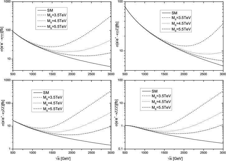
Figure 2: The cross sections for the process $e^{-}e^{+}\to VVV$ with $V=\gamma,Z$ in the SM and LED model as the function of $\sqrt{s}$ with $M_{s}=$ 3.5, 4.5, 5.5 TeV and $\delta=3$.

In Fig.3 we present the dependence of the cross section on energy scale $M_{S}$ with $\sqrt{s}=1$ TeV, 2 TeV and 3 TeV respectively. In each figure of Fig.3, we present the curves for the cross sections with the extra dimension $\delta$ value being 3, 4, 5 and 6 separately. The solid straight lines, which are independent of $M_{S}$, are the SM results, and the dashed, dotted, dash-dotted and dash-dot-dotted lines are the cross sections for $\delta$=3, 4, 5 and 6 respectively. It’s clear that for a given value of $\delta$, the cross section decreases rapidly with the increment of $M_{S}$, and finally approaches to its corresponding SM result. We can see again that the virtual KK graviton exchange contribution decreases with the increment of the $\delta$ value. The LED effect on the cross sections with $\sqrt{s}=1$ TeV is too small to be detected, especially for $e^{-}e^{+}\to\gamma\gamma Z$ process, which is coincidence with Fig.2. If we got high enough c.m.s energy, say 3 TeV, the cross sections would be very significant when $M_{S}$ is not very large. Even with $M_{S}=6$ TeV, the cross sections are still several times of the SM ones.

Figure 3: The cross sections for the process $e^{-}e^{+}\rightarrow VVV$ in the SM and LED model as the function of $M_{S}$ with $\sqrt{s}=$ 1, 2, 3 TeV and $\delta=3,~{}4,~{}5,~{}6$.

3.3 Distributions

The distributions of the Gauge boson pair invariance mass $M_{VV}$ ($VV=\gamma\gamma,~{}ZZ$) and the Gauge boson transverse momentum $p_{T}^{V}$ as well as their rapidity $y^{V}$ at the 3 TeV CILC, are shown in Fig.4-6. The results are for $M_{S}=6.5$ TeV at the fixed value 4 for the number of extra dimensions and obtained by taking the input parameters mentioned above.

$e^{-}e^{+}\rightarrow\gamma\gamma\gamma$

Before selecting our event samples for triple $\gamma$ production, we order the photons on the basis of their transverse momentum i.e., $p_{T}^{\gamma_{1}}\geq p_{T}^{\gamma_{2}}\geq p_{T}^{\gamma_{3}}$. For $e^{-}e^{+}\rightarrow\gamma\gamma\gamma$, we are interested in the $p_{T}^{\gamma}$ and $y^{\gamma}$ distribution which are displayed in the left and right panel in Fig.4, respectively. The solid, dashed and dotted lines refer to $\gamma_{1}$, $\gamma_{2}$ and $\gamma_{3}$, respectively. In high $p_{T}^{\gamma_{1}}$ and $p_{T}^{\gamma_{2}}$ region, the LED effect dominant the total (SM+LED) distribution, because more KK modes contribute with the increase of $p_{T}$. Difference can be found for the $p_{T}^{\gamma_{3}}$ production, although it’s still enhanced by the LED effects, it’s low $p_{T}$ region is dominant while in high $p_{T}$ region it becomes much smaller. Rapidity distribution of the related photon has been shown in the right panel in Fig.4. As we can see, the rapidity distributions in the LED model show significantly peaks around $y=0$, which implies the large contributions at high $p_{T}^{\gamma_{1,2}}$ region. Compare with the $\gamma_{1}$ and $\gamma_{2}$ distribution, the $y$ distribution of $\gamma_{3}$ seems much flatter.

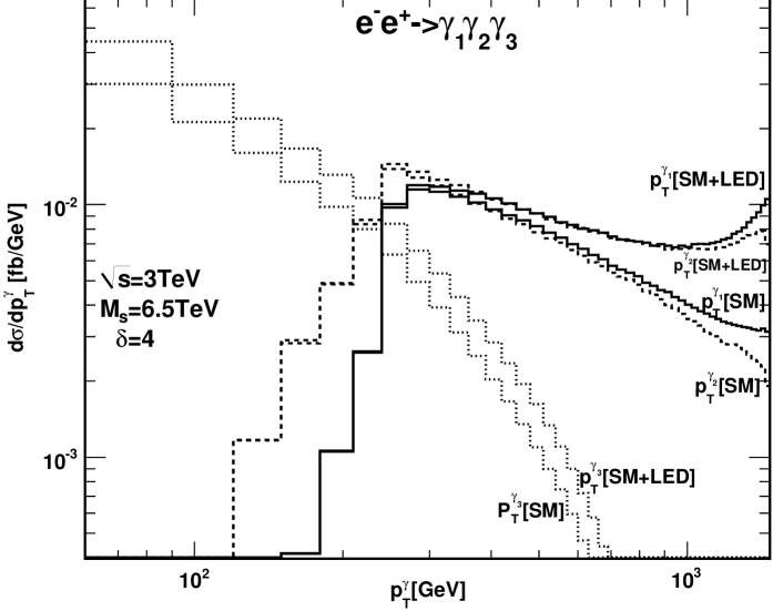
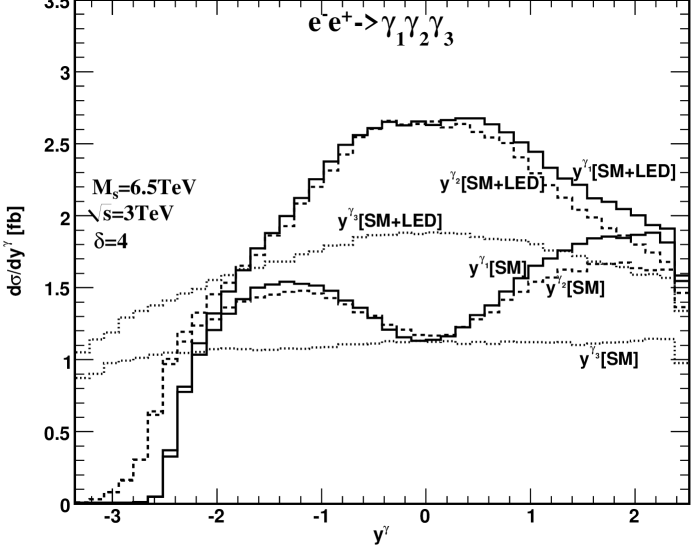
Figure 4: The transverse momentum($p_{T}$) and Rapidity($y$) distribution of photons for the process $e^{-}e^{+}\rightarrow\gamma\gamma\gamma$, on the basis of their transverse momentum $p_{T}^{\gamma_{1}}\geq p_{T}^{\gamma_{2}}\geq p_{T}^{\gamma_{3}}$ with $M_{S}=$ 6.5TeV, $\sqrt{s}=$3 TeV and $\delta=4$. The solid, dashed and dotted lines refer to $p_{T}^{\gamma_{1}}$($y^{\gamma_{1}}$), $p_{T}^{\gamma_{2}}$($y^{\gamma_{2}}$) and $p_{T}^{\gamma_{3}}$($y^{\gamma_{3}}$).

$e^{-}e^{+}\rightarrow ZZZ$

Similar to the $e^{-}e^{+}\rightarrow\gamma\gamma\gamma$ production, triple Z bosons final particles are classified in such a way that $p_{T}^{Z_{1}}\geq p_{T}^{Z_{2}}\geq p_{T}^{Z_{3}}$. Similar conclusion can be found for the $e^{-}e^{+}\rightarrow ZZZ$ production. It’s not strange that the signal of triple $\gamma$ signal is larger than the triple Z production since the three Z bosons suppress the phase space integration extremely, so that the total cross sections as well as the distributions become smaller as can be seen in Fig.4 and Fig.5, the peak is around 0.0006 fb/GeV for $p_{T}^{Z_{1}}$ compared to 0.01 fb/GeV for $p_{T}^{\gamma_{1}}$ in the high $p_{T}$ region. For the $y$ distributions, the peaks for the $ZZZ$ production are narrower than the $\gamma\gamma\gamma$ distributions, however, the conclusion is the same that the rapidity distributions in the LED model show significant peaks around $y=0$.

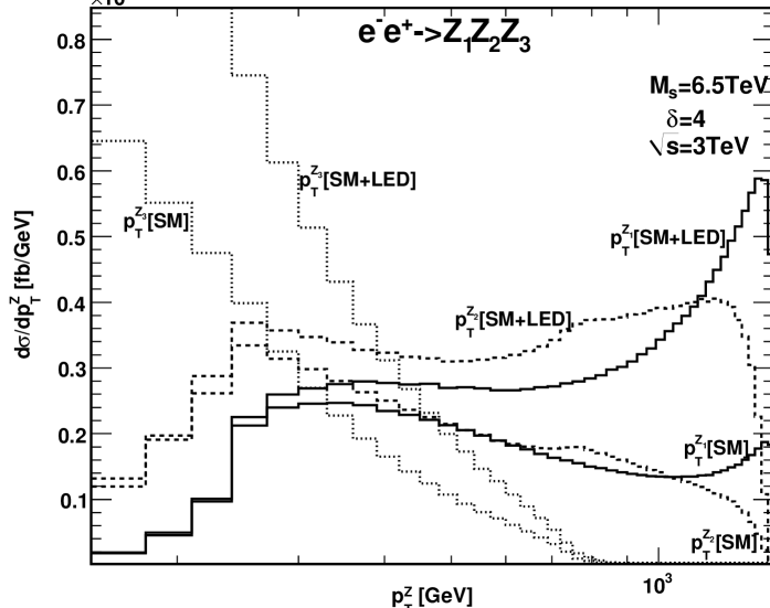
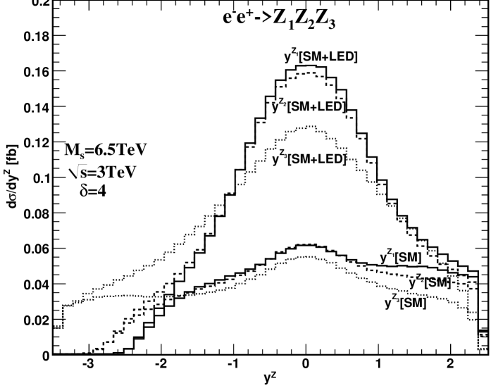
Figure 5: The transverse momentum($p_{T}$)and Rapidity($y$) distribution of $Z$ bosons for the process $e^{-}e^{+}\rightarrow ZZZ$, on the basis of their transverse momentum $p_{T}^{Z_{1}}\geq p_{T}^{Z_{2}}\geq p_{T}^{Z_{3}}$ with $M_{S}=6.5$ TeV, $\sqrt{s}=3$ TeV and $\delta=4$. The solid, dashed and dotted lines refer to $p_{T}^{Z_{1}}$($y^{Z_{1}}$), $p_{T}^{Z_{2}}$($y^{Z_{2}}$) and $p_{T}^{Z_{3}}$($y^{Z_{3}}$).

$e^{-}e^{+}\rightarrow\gamma\gamma Z$ and $e^{-}e^{+}\rightarrow\gamma ZZ$

Now let’s see the distributions for the $e^{-}e^{+}\rightarrow\gamma\gamma Z$ and $e^{-}e^{+}\rightarrow\gamma ZZ$ productions. The photon pair decay of the KK graviton is one of the clean decay modes, so the distribution of the invariant mass of the photon pair ($M_{\gamma\gamma}$) is a useful observable for $e^{-}e^{+}\to\gamma\gamma Z$ . An obvious enhancement on the tail of this distribution makes such region of extreme interest. Typically, we find that the KK modes dominate over SM contribution for larger values of invariant masses (say above 1 TeV for a given set of $M_{S}$ and $\delta$ values, here we give $M_{S}=4.5$ TeV and $\delta=4$) of photon pairs indicating the observable nature of the signal, see the two dotted line in Fig.6. The upper and lower ones refer to the SM predict and SM+LED effects. For the process $e^{-}e^{+}\rightarrow\gamma ZZ$, it is similar to $\gamma\gamma Z$ production process, and in this case, the invariant mass of Z boson pair($M_{ZZ}$) is a useful observable. We thus display it in Fig.6, see the solid lines. These two solid line branch at about the invariance mass 1 TeV, and the upper and lower ones present the SM and SM+LED effects, respectively.

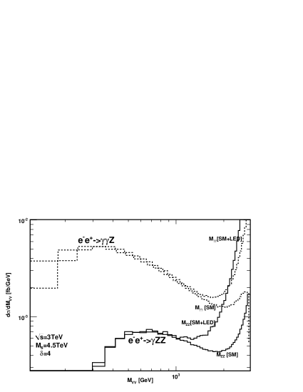
Figure 6: Invariant mass distribution of $M_{\gamma\gamma(ZZ)}$ for $e^{-}e^{+}\rightarrow\gamma\gamma Z$($e^{-}e^{+}\rightarrow\gamma ZZ$) for $M_{S}=4.5$ TeV, $\sqrt{s}=3$ TeV and $\delta=4$.

It is clear that if the deviation of the cross section from the SM prediction is large enough, the LED effects can be found. We assume that the LED effects can and cannot be observed, only if[35]

$$\Delta\sigma=|\sigma_{tot}-\sigma_{SM}|\geq\frac{5\sqrt{{\cal L}\sigma_{tot}}}{{\cal L}}\equiv 5\sigma$$ (8)

and

$$\Delta\sigma=|\sigma_{tot}-\sigma_{SM}|\leq\frac{3\sqrt{{\cal L}\sigma_{tot}}}{{\cal L}}\equiv 3\sigma$$ (9)

$\sqrt{s}$		1 TeV			2 TeV			3 TeV
		$5\sigma$	$3\sigma$		$5\sigma$	$3\sigma$		$5\sigma$	$3\sigma$
$e^{-}e^{+}\rightarrow\gamma\gamma\gamma$		3599	4093		6371	7187		8906	10023
$e^{-}e^{+}\rightarrow ZZZ$		2530	2858		4711	5312		6730	7584
$e^{-}e^{+}\rightarrow\gamma\gamma Z$		2052	2289		4007	4458		5823	6500
$e^{-}e^{+}\rightarrow\gamma ZZ$		3406	3835		6027	6757		8412	9421

Table 1: The discovery ($\Delta\sigma\geq 5\sigma$) and exclusion ($\Delta\sigma\leq 3\sigma$) LED model fundamental scale ($M_{S}$) values for the $e^{-}e^{+}\to VVV$ processes at the $\sqrt{s}$ = 1, 2, 3 TeV ILC(CLIC). ${\cal L}=300~{}{\rm fb}^{-1}$, $\delta=4$.

Our final results show that by using the $\gamma\gamma\gamma$ production we can set the discovery limit on the fundamental Plank scale $M_{S}$ up to 3.1-9.9 TeV, depending on the extra dimension $\delta\subset[3,6]$, with the luminosity 300 fb^-1 and the colliding energy 1-3 TeV. For the other three final states $\gamma\gamma Z$ , $\gamma ZZ$ and $ZZZ$ , the limits are 1.8-6.3 TeV, 2.9-9.3 TeV and 2.2-7.4 TeV, respectively. To do a more detailed description, in Table 1, we present the $5\sigma$ discovery and $3\sigma$ exclusion fundamental scale $M_{S}$ values at the ILC/CLIC with the luminosity 300 fb^-1 for $\delta=4$ . It shows that compared to the other three channels, $\gamma\gamma\gamma$ can set the discovery limit bounds much higher, up to 8.9 TeV. The phenomenology of the neutral triple gauge boson production at the near future is much richer at linear colliders, though its production cannot give compete limits as, for example, dilepton production gives, it’s still very interesting and important.

		${\cal L}$ (${\rm fb}^{-1}$)
		$5\sigma$	$3\sigma$
$pp\rightarrow\gamma\gamma\gamma$		960	1500
$pp\rightarrow ZZZ$		21	21
$pp\rightarrow\gamma\gamma Z$		20	17
$pp\rightarrow\gamma ZZ$		170	140

Table 2: Integrated luminosity needed at 14 TeV LHC to accomplish the discovery and exclusion bounds at a 1 TeV linear collider, which are listed in the first two columns in Table 1, using the neutral triple gauge boson production processes, with $\delta=4$.

To make a comparison with Ref.[26], we repeat the $pp\to VVV$ ($V=\gamma,Z$) process at LHC, using the same parameters and cuts with Ref.[26], and find that our results are in good agreement with theirs. In Table 2 we list the integrated luminosity the 14 TeV LHC needed to accomplish the discovery and exclusion bounds at a 1 TeV LC (the first two column data listed in Table 1), by using the corresponding $VVV$ production channels with extra dimensions $\delta=4$. The table shows that with years of collection of data, LHC could accomplish the discovery and exclusion limits set by a 1 TeV LC, even for the most challenging channel $\gamma\gamma\gamma$ . While the limits set by a 2 or 3 TeV LC are much higher, and the required amounts of data for matching these bounds are too large to be a reasonable projection for the LHC reach.

4 Summary and Conclusions

In a short summary, we calculate the neutral gauge boson production processes $\gamma\gamma\gamma$, $\gamma\gamma Z$, $\gamma ZZ$ and $ZZZ$ in the SM and LED model at ILC and CLIC. We investigate the integrated cross sections, the distributions of some kinematic variables $M_{VV}$, $p_{T}^{V}$ and $y^{V}$. The 5$\sigma$ discovery and 3$\sigma$ exclusion ranges for the LED parameters $M_{S}$ are obtained and compared between different channels. It turns out that the effects of the virtual KK graviton enhance the total cross sections and differential distributions of kinematical observables generally. Among the four processes we considered, $e^{-}e^{+}\to\gamma ZZ$ or $e^{-}e^{+}\to\gamma\gamma\gamma$ process has the most significant LED effect with relatively small or large $M_{S}$, respectively. While $e^{-}e^{+}\to\gamma\gamma Z$ has the least contribution from LED diagrams. With the development of linear colliders, more information related to LED effects can be obtained experimentally through such important productions. At the 3 TeV CLIC, it is expected that $\gamma ZZ$ production can be used to explore a range of $M_{S}$ values up to 7.3-9.3 TeV depending on the number of extra dimensions. Through $\gamma\gamma\gamma$ production, we can extend this search up to 9.9 TeV, While using $\gamma\gamma Z$ and $ZZZ$ productions, lower bounds on $M_{S}$ can be found, which are 6.3 TeV and 7.4 TeV, respectively.

5 Acknowledgments

We would like to thank Prof. Zhang Ren-You for useful discussions. Project supported by the National Natural Science Foundation of China (Grant No.11147151, No.11205070, No.11105083, No.10947139 and No.11035003), and by Shandong Province Natural Science Foundation (No.ZR2012AQ017).

References

- [1] N. Arkani-Hamed, S. Dimopoulos and G. R. Dvali, Phys. Lett. B 429, 263 (1998) [hep-ph/9803315]; N. Arkani-Hamed, S. Dimopoulos and G. R. Dvali, Phys. Rev. D 59, 086004 (1999) [hep-ph/9807344].
- [2] D. J. Kapner, T. S. Cook, E. G. Adelberger, J. H. Gundlach, B. R. Heckel, C. D. Hoyle and H. E. Swanson, Phys. Rev. Lett. 98, 021101 (2007) [arXiv:hep-ph/0611184].
- [3] Gian F. Giudice, Riccardo Rattazzi, James D. Wells, Nucl.Phys. B544, 3-38 (1999).
- [4] Tao Han, Joseph D. Lykken, Ren-Jie Zhang, Phys.Rev.D59:105006(1999).
- [5] J. L. Hewett, Phys. Rev. Lett. 82 (1999) 4765; Prakash Mathews, V. Ravindran, K. Sridhar and W. L. van Neerven, Nucl. Phys. B713 (2005) 333; Prakash Mathews, V. Ravindran, Nucl. Phys. B753 (2006) 1; M.C. Kumar, Prakash Mathews, V. Ravindran, Eur. Phys. J. C49 (2007) 599.
- [6] O. J. P. Eboli, Tao Han, M. B. Magro, P. G. Mercadante, Phys. Rev. D61 (2000) 094007; K.m. Cheung and G. L. Landsberg, Phys. Rev. D 62 (2000) 076003; M.C. Kumar, Prakash Mathews, V. Ravindran, Anurag Tripathi, Phys. Lett. B672 (2009) 45; Nucl. Phys. B818 (2009) 28.
- [7] M. Kober, B. Koch and M. Bleicher, Phys. Rev. D 76, 125001 (2007) [arXiv:0708.2368]; J. Gao, C. S. Li, X. Gao and J. J. Zhang, Phys. Rev. D 80, 016008 (2009) [arXiv:0903.2551]; Neelima Agarwal, V. Ravindran, V. K. Tiwari, Anurag Tripathi, Nucl. Phys. B830 (2010) 248.
- [8] Z. U. Usubov and I. A. Minashvili, Phys. Part. Nucl. Lett. 3, 153 (2006) [Pisma Fiz. Elem. Chast. Atom. Yadra 3, 24 (2006)]; K. Y. Lee, H. S. Song and J. -H. Song, Phys. Lett. B 464, 82 (1999) [hep-ph/9904355]. Neelima Agarwal, V. Ravindran, V. K. Tiwari, Anurag Tripathi, Phys. Rev. D82 (2010) 036001; B. Yu-Ming, G. Lei, L. Xiao-Zhou, M. Wen-Gan and Z. Ren-You, Phys. Rev. D 85, 016008 (2012) [arXiv:1112.4894].
- [9] Prakash Mathews, Sreerup Raychaudhuri, K. Sridhar, Phys. Lett. B450 (1999) 343; JHEP 0007 (2000) 008.
- [10] K. Y. Lee, H. S. Song, J. -H. Song and C. Yu, Phys. Rev. D 60, 093002 (1999) [hep-ph/9905227]; K. Y. Lee, S. C. Park, H. S. Song, J. -H. Song and C. Yu, Phys. Rev. D 61, 074005 (2000) [hep-ph/9910466]; hep-ph/0105326; S. C. Inan and A. A. Billur, Phys. Rev. D 84, 095002 (2011).
- [11] C. S. Kim, Kang Young Lee and Jeonghyeon Song, Phys.Rev.D64:015009(2001); A. Datta, E. Gabrielli and B. Mele, JHEP 0310, 003 (2003) [hep-ph/0303259]; Hao Sun, Ya-Jin Zhou, He Chen, Eur. Phys. J. C (2012) 72:2011.
- [12] E. A. Mirabelli, M. Perelstein and M. E. Peskin, Phys. Rev. Lett. 82, 2236 (1999) [hep-ph/9811337].
- [13] K. -m. Cheung and W. -Y. Keung, Phys. Rev. D 60, 112003 (1999) [hep-ph/9903294].
- [14] C. Collaboration [CMS Collaboration], arXiv:1204.0821 [hep-ex].
- [15] S. Chatrchyan et al. [CMS Collaboration], Phys. Lett. B 711, 15 (2012) [arXiv:1202.3827 [hep-ex]].
- [16] S. Chatrchyan et al. [CMS Collaboration], arXiv:1112.0688 [hep-ex].
- [17] M. Golden and S. R. Sharpe, Nucl. Phys. B 261, 217 (1985).
- [18] V. D. Barger and T. Han, Phys. Lett. B 212, 117 (1988).
- [19] Tao Han and Ron Sobey, Phys.Rev. D52 (1995) 6302-6308.
- [20] Fawzi Boudjema, Le Duc Ninh, Sun Hao, Marcus M. Weber, Phys.Rev.D81 (2010)073007; Fortsch. Phys.58 :656-659 (2010);
- [21] Su Ji-Juan, Ma Wen-Gan, Zhang Ren-You, Wang Shao-Ming, Guo Lei, Phys.Rev.D78(2008)016007;
- [22] Sun Wei, Ma Wen-Gan, Zhang Ren-You, Guo Lei, Song Mao, Phys.Lett.B680(2009)321-327;
- [23] T. Binoth, G. Ossola, C.G. Papadopoulos, R. Pittau, JHEP 0806 (2008) 082;
- [24] A. Lazopoulos, K. Melnikov, F. Petriello, Phys. Rev. D 76 (2007) 014001;
- [25] G. Bozzi, F. Campanario, V. Hankele, D. Zeppenfeld, Phys. Rev. D 81 (2010) 094030; G. Bozzi, F. Campanario, M. Rauch, D. Zeppenfeld, Phys. Rev. D 84 (2011) 074028.
- [26] M. C. Kumar, Prakash Mathews, V. Ravindran, Satyajit Seth, DESY 11-229, [arXiv:1111.7063].
- [27] G. Aarons et al. [ILC Global Design Effort and World Wide Study], International Linear Collider Reference Design Report Volume 2: Physics at the ILC, edited by A. Djouadi, J. Lykken, K. Mig, Y. Okada, M. Oreglia and S. Yamashita, arXiv:0709.1893.
- [28] L. Linssen, A. Miyamoto, M. Stanitzki and H. Weerts (editors), Physics and Detectors at CLIC : the CLIC Conceptual Design Report, arXiv:1202.5940 [physics.ins-det].
- [29] T. Hahn, Comput.Phys.Commun. 140, 418-431 (2001).
- [30] T. Hahn, Nucl.Phys.Proc.Suppl. 89, 231-236 (2000).
- [31] S. Kawabata, Comp. Phys. Commun. 88, 309 (1995). F. Yuasa, D. Perret-Gallix, S. Kawabata, and T. Ishikawa, Nucl. Instrum. Meth. A389, 77 (1997).
- [32] Particle Data Group, K. Nakamura et al., JPG 37, 075021 (2010).
- [33] G. Aad et al. [ATLAS Collaboration],CERN-PH-EP-2012-218, [arXiv:1207.7214 [hep-ex]].
- [34] S. Chatrchyan et al. [CMS Collaboration],CMS-HIG-12-028, CERN-PH-EP-2012-220, [arXiv:1207.7235 [hep-ex]].
- [35] Sun Hao, Zhang Ren-You, Zhou Pei-Jun, Ma Wen-Gan, Jiang Yi and Han Liang, Phys.Rev. D71, 075005 (2005)