Generalized Lüscher Formula in Multi-channel Baryon-Meson Scattering

Abstract

Lüscher’s formula relates the elastic scattering phase shifts to the two-particle energy levels in a finite cubic box. The original formula was obtained for elastic scattering of two massive spinless particles in the center of mass frame. In this paper, we consider the case for the scattering of a spin $1/2$ particle with a spinless particle in multi-channel scattering. A generalized relation between the energy of two particle system and the scattering matrix elements is established. We first obtain this relation using quantum-mechanics in both center-of-mass frame and in a general moving frame. The result is then generalized to quantum field theory using methods outlined in Ref. Hansen and Sharpe (2012). We verify that the results obtained using both methods are equivalent up to terms that are exponentially suppressed in the box size.

I INTRODUCTION

Low-energy hadron-hadron scattering plays an important role for the understanding of strong interaction. However, due to its non-perturbative nature, it should be studied using a non-perturbative method like lattice Chromodynamics (lattice QCD). Lattice QCD can tackle the problem from first principles of QCD using numerical simulations. By measuring appropriate correlation functions, energy eigenvalues of two-particle states in a finite box can be obtained. Lüscher found out a relation, now commonly known as Lüscher’s formula, which relates the energy of two-particle state in a finite box of size $L$, $E(L)$, to the elastic scattering phase $\delta(E(L))$ of the two particles in the continuum Lüscher (1986); Lüscher and Wolff (1990); Lüscher (1991a, b). While the former could be obtained in lattice QCD simulations, the latter fully characterizes the scattering property of the two particles and could in principle be measured in corresponding experiments. Thus, this relation opens up the possibility of lattice study of hadron-hadron scattering.

Lüscher’s formalism has been utilized in a number of lattice applications, e.g. linear sigma model in broken phase Gockeler et al. (1994), hadron-hadron scattering both with quenched approximation and unquenched configuration that contains dynamic quarks Gupta et al. (1993); Fukugita et al. (1995); Aoki et al. (2000, 2002); Liu et al. (2002); Hasenfratz et al. (2004); Du et al. (2004); Aoki et al. (2005, 2003); Yamazaki et al. (2004); Beane et al. (2006a).However, the original Lüscher’s method is restricted to elastic scattering of massive, spinless particles in the center-of-mass (COM) frame of the two particles. Some of these constraints restrain the applicability of the formalism to general hadron scattering. For example, in real simulations, one is usually restricted to only a few lattice volumes and since the energies in the box is quantized, and taking into account the fact that excited energy states are more difficult to measure numerically, one ends up with a rather poor energy resolution when compared with the experiments. To overcome this difficulty, one can of course consider asymmetric volumes Li and Liu (2004); Feng et al. (2004); Li et al. (2007), or boosting the system to a frame that is different from COM Rummukainen and Gottlieb (1995); Xu Feng (2011); Davoudi and Savage (2011); Fu (2012); Gockeler et al. (2012), both will enhance the energy resolution of the problem. Another possible generalization is to use the so-called twisted boundary conditions advocated in Refs. Bedaque and Chen (2005); Bedaque (2004); Sachrajda and Villadoro (2005); de Divitiis et al. (2004).

Generalizations to particles with spin Beane et al. (2006b, 2004); Meng et al. (2004) is also possible. For example, in Ref. Bernard et al. (2008); Ishizuka (2009), Lüscher’s formula has been extended to elastic scattering of baryons.

It is also important to extend Lüscher’s formula to the case of inelastic scattering which is commonly encountered in hadronic physics. Attempts have been made over the years, see Refs. He et al. (2005); Liu et al. (2006); Lage et al. (2009a); Ishii and Collaboration (2011); Aoki et al. (2011); Hansen and Sharpe (2012); Doring et al. (2011, 2012).

In this paper, we would like to synthesize the above mentioned generalizations by trying to seek a formula (or a formalism) that is applicable for multi-channel scattering of particles with spin in a possibly moving frame (MF). For this purpose, we consider two-particle to two-particle scattering processes in which one particle has spin $1/2$ (we will henceforth call it a “baryon”) while the other particle remains spinless (we will call it a “meson”). The scattering process we study could be a multi-channel scattering beyond a certain threshold. But in each channel, the two-particle states (initial or final) always has the feature that one particle has spin $1/2$ while the other is spinless. We will comment on possible extensions to this restriction in Sec. IV. As it turns out, the basic formulae obtained are the same in non-relativistic quantum mechanics and in massive quantum field theories, we will start our discussion in the former case. Generalization to quantum field theory can be achieved by using methods outlined in Refs. Ishizuka (2009); Hansen and Sharpe (2012) which is detailed in Sec. III.

The organization of the paper is as follows: In Sec. II, we start out by discussing a quantum-mechanical model. Lüscher’s formulae are obtained first in the case of COM frame in subsection II.1 and then generalize to moving frames in subsection II.2. In Sec. III, we generalize the results obtained in Sec. II to quantum field theory. This is achieved first in the single channel situation and then to the two-channel scenario. We then compare the results obtained in quantum field theory with those from quantum mechanics in Sec. II. It is shown that they are in fact equivalent up to terms that are exponentially suppressed in the large volume limit. In Sec. IV, before we conclude, we will also discuss possible applications of our formulae in real lattice simulations and comment on some possible extensions in the future.

Some calculation details are summarized in the appendices. To be more specific, single channel scattering for particles with spin in infinite volume are reviewed in appendix A. For reference, single channel Lüscher’s formulae are also provided in this appendix. Calculations of loop summation/integration in the case of quantum field theory are summarized in appendix B.

II Lüscher’s formula for baryon-meson scattering in non-relativistic quantum mechanics

II.1 Lüscher’s formula in COM frame

II.1.1 Two-channel scattering in the continuum

In this section, using non-relativistic quantum mechanics in COM frame, we will briefly discuss two-channel potential scattering in the continuum for the case of two stable particles: one with spin $0$ (a meson) and the other with spin $\frac{1}{2}$ (a baryon). We will follow the discussion in Ref. He et al. (2005). The potential $V(r)$ between the two particles is assumed to have finite range, i.e., $V(r)=0$ with $r=|\mathbf{r}|>R$ for some positive $R$, but the potential itself could in principle be spin-dependent so that the spin of the fermion might change during the scattering process. We assume that there exists a threshold $E_{T}>0$ and the energy of the two-particle system becomes

$$E = {\mathbf{k}^{2}_{1}\over 2\mu_{1}}=E_{T}+{\mathbf{k}^{2}_{2}\over 2\mu_{2}}\;,$$ (1)

where $\mu_{1}$ and $\mu_{2}$ are the reduced mass of the two-particle system below and above the threshold, respectively. In the COM frame, one only has to denote the momentum of one of the two particles. For definiteness, we denote the momentum of the fermion as $\mathbf{k}_{1}$ and $\mathbf{k}_{2}$ in the first and second channel, respectively. The magnitude of them are $k_{1}=|\mathbf{k}_{1}|$ and $k_{2}=|\mathbf{k}_{2}|$. Obviously, for energies below the threshold $k_{2}$ will become pure imaginary.

The wave function of two-particle system, after factoring out the trivial COM coordinates, has a two-component form in the case of two-channel scattering: He et al. (2005)

$$\psi(\mathbf{r}) = \left(\begin{array}[c]{c}\psi_{1}(\mathbf{r})\\ \psi_{2}(\mathbf{r})\end{array}\right)\;.$$ (4)

Note that due to spin degrees of freedom, each component is still a two-component spinor. At large $r$ where the potential $V(r)$ vanishes, the wave functions of the scattering states can be chosen to have the following forms:

$$\psi_{1;s}(\mathbf{r})\overset{r\rightarrow\infty}{\longrightarrow}\left(\begin{array}[]{c}\chi^{\frac{1}{2}}_{s}e^{i\mathbf{k_{1}\cdot{r}}}+\sum_{s^{\prime}}\chi^{\frac{1}{2}}_{s^{\prime}}M^{(NR)}_{11;s^{\prime}s}\frac{e^{ik_{1}r}}{r}\\ \sqrt{\frac{\mu_{2}}{\mu_{1}}}\sum_{s^{\prime}}\chi^{\frac{1}{2}}_{s^{\prime}}M^{(NR)}_{21;s^{\prime}s}\frac{{e^{ik_{2}r}}}{r}\end{array}\right)\;,$$ (7)

$$\psi_{2;s}(\mathbf{r})\overset{r\rightarrow\infty}{\longrightarrow}\left(\begin{array}[]{c}\sqrt{\frac{\mu_{1}}{\mu_{2}}}\sum_{s^{\prime}}\chi^{\frac{1}{2}}_{s^{\prime}}M^{(NR)}_{12;s^{\prime}s}\frac{{e^{ik_{1}r}}}{r}\\ \chi_{s}^{\frac{1}{2}}e^{i\mathbf{k_{2}\cdot{r}}}+\sum_{s^{\prime}}\chi^{\frac{1}{2}}_{s^{\prime}}M^{(NR)}_{22;s^{\prime}s}\frac{e^{ik_{2}r}}{r}\end{array}\right)\;.$$ (10)

In the above expressions, $\chi^{\frac{1}{2}}_{s}$ is an eigenstate of spin angular momentum $s_{z}$ of the baryon with eigenvalue $s=-1/2,1/2$. The scattering amplitudes like $M^{(NR)}_{ij;s^{\prime}s}$ depends only on the corresponding angles $\hat{\mathbf{k}}_{1}\cdot\hat{\mathbf{r}}$ and $\hat{\mathbf{k}}_{2}\cdot\hat{\mathbf{r}}$. In order not to confuse with the matrix $M$ introduce in quantum field theory in Sec. III, we have added a superscript (NR) to stand for the case of non-relativistic quantum mechanics. The notation in this paper is as follows. Subscripts like $i$ and $j$ refer to the channel, and take the values 1 or 2. It is seen that, in the remote past, $\psi_{1;s}(\mathbf{r})$ becomes a pure incident plane wave in the first channel with definite linear momentum $\mathbf{k_{1}}$ and definite spin $s$. Similarly, in the remote past, $\psi_{2;s}(\mathbf{r})$ represents an incident plane wave in the second channel with definite momentum $\mathbf{k}_{2}$ and definite spin $s$. It is also clear that the above wave functions, $\psi_{i;s}(\mathbf{r})$ with $s=-1/2,1/2$ are linearly independent and in fact they are also complete in the sense that any eigenfunction of the Hamiltonian must be a linear superposition of them.

As is said, the scattering amplitudes $M^{(NR)}_{ij;s^{\prime}s}$ for $s^{\prime},s=1/2,-1/2$ depend only on the corresponding angles and can be expanded into spherical harmonics, see for example Ref. Newton (1982). For simplicity, we have chosen the $z$-axis to coincide with the incident momentum, $\mathbf{k}_{1}$ and $\mathbf{k}_{2}$ for $\psi_{1;s}(\mathbf{r})$ and $\psi_{2;s}(\mathbf{r})$, respectively. The scattering amplitudes then takes the following form:

$$M^{(NR)}_{11;s^{\prime}s}(\mathbf{\hat{k}_{1}\cdot{\hat{r}}}) = \frac{1}{2ik_{1}}\sum_{l=0}^{\infty}\sum_{J=l-\frac{1}{2}}^{l+\frac{1}{2}}\sqrt{4\pi(2l+1)}(S_{11}^{Jl}-1)S^{l\frac{1}{2}}_{JM;ms^{\prime}}S^{l\frac{1}{2}}_{JM;0s}Y_{lm}(\mathbf{\hat{r}})\;,$$ (11)

$$M^{(NR)}_{12;s^{\prime}s}(\mathbf{\hat{k}_{2}\cdot{\hat{r}}}) = \frac{1}{2i\sqrt{k_{1}k_{2}}}\sum_{l=0}^{\infty}\sum_{J=l-\frac{1}{2}}^{l+\frac{1}{2}}\sqrt{4\pi(2l+1)}{S^{Jl}_{12}}S^{l\frac{1}{2}}_{JM;ms^{\prime}}S^{l\frac{1}{2}}_{JM;0s}Y_{lm}(\mathbf{\hat{r}})\;.$$ (12)

In the above expressions, $S_{JM;ms^{\prime}}^{l\frac{1}{2}}=\langle{JM}|lm;\frac{1}{2}s^{\prime}\rangle$ and $S_{JM;0s}^{l\frac{1}{2}}=\langle{JM}|l0;\frac{1}{2}s\rangle$ are the Clebsch-Gordan (CG) coefficients.

The quantities $S^{Jl}_{ij}$ are the $S$-matrix elements where $J$ is the quantum number of the total angular momentum. Since we are dealing with the scattering of a spin $1/2$ particle, $J$ can take two possible values for a given $l$, namely $J=l\pm 1/2$. To simplify the notation we will also denote the corresponding $S$-matrix elements by

$$S^{J=l\pm 1/2,l}_{ij}\equiv S^{l\pm}_{ij}\;.$$ (13)

Needless to say, one also has similar expressions for $M^{(NR)}_{21;s^{\prime}s}$ and $M^{(NR)}_{22;s^{\prime}s}$. In the following, we will also need the so-called spin spherical harmonics defined as

$$Y_{JM}^{l\frac{1}{2}}(\mathbf{\hat{r}})=\sum_{ms}Y_{lm}(\mathbf{\hat{r}})\chi_{s}^{\frac{1}{2}}S_{JM;ms}^{l\frac{1}{2}}\;,$$ (14)

which is an eigenfunction of the total angular momentum of the system. The above expressions are just direct generalizations to the spin-dependent single-channel scattering. For convenience, some relevant formulae are collected in appendix A.

With the spin spherical harmonics defined in Eq. (14), we can expand the wave function in the following form:

$$\psi_{i;s}(\mathbf{r})=\sum_{JMl}\sqrt{4\pi(2l+1)}S_{JM;0s}^{l\frac{1}{2}}W_{i;Jl}(r)Y_{JM}^{l\frac{1}{2}}(\mathbf{\hat{r}})\;,$$ (15)

where the radial wave functions of Schrödinger equation are denoted by $W_{i;Jl}(r)$. In the large $r$ region, they have the following asymptotic forms

$$W_{1;Jl}(r) = \left(\begin{array}[c]{c}\frac{1}{2ik_{1}r}[S^{Jl}_{11}e^{ik_{1}r}+(-1)^{l+1}e^{-ik_{1}r}]\\ \frac{1}{2ir\sqrt{k_{1}k_{2}}}\sqrt{\frac{\mu_{2}}{\mu_{1}}}S^{Jl}_{21}e^{ik_{2}r}\end{array}\right)\;,$$ (18)

$$W_{2;Jl}(r) = \left(\begin{array}[c]{c}\frac{1}{2ir\sqrt{k_{1}k_{2}}}\sqrt{\frac{\mu_{1}}{\mu_{2}}}S^{Jl}_{12}e^{ik_{1}r}\\ \frac{1}{2ik_{2}r}[S^{Jl}_{22}e^{ik_{2}r}+(-1)^{l+1}e^{-ik_{2}r}]\end{array}\right)\;.$$ (22)

It is obvious that two radial wave functions $W_{1;Jl}(r)$ and $W_{2;Jl}(r)$ are linearly independent. Since the radial Schrödinger equation has two linearly independent solutions which are regular at the origin, denoted by $u_{i;Jl}(r)$, these radial wave functions can be expressed as linear superpositions of two radial wave functions $W_{i;Jl}(r)$ He et al. (2005).

II.1.2 Two-channel scattering in a cubic box

Now we put the two-particle system into a cubic box of size $L$ and impose the periodic boundary condition. The potential then becomes $V_{L}(\mathbf{r})=\sum\nolimits_{\mathbf{n}}V(\mathbf{r}+\mathbf{n}L)$, $\mathbf{n}\in\mathbbm{Z}^{3}$. We divide the whole space into two regions: the inner region and the outer region. In the inner region, every point satisfy the condition: $|\mathbf{r}+\mathbf{n}L|<R$, for some $\mathbf{n}\in\mathbbm{Z}^{3}$ while in the outer region, $\Omega=\{\mathbf{r}|:|\mathbf{r}+\mathbf{n}L|>R$, $\mathbf{n}\in\mathbbm{Z}^{3}\}$. In the inner region, the solution to Schrödinger equation of the system is

$$\psi(\mathbf{r})=\sum_{l=0}^{\infty}\sum_{J=l-\frac{1}{2}}^{l+\frac{1}{2}}\sum_{M=-J}^{J}\left[\sum_{i=1}^{2}b_{i;JMl}u_{i;Jl}(r)\right]Y_{JM}^{l\frac{1}{2}}(\mathbf{\hat{r}})\;.$$ (24)

Since $u_{i;Jl}(r)$ can be expressed as linear superpositions of two radial wave functions $W_{i;Jl}(r)$, in the outer region the wave function is given by

$$\psi(\mathbf{r})=\sum_{l=0}^{\infty}\sum_{J=l-\frac{1}{2}}^{l+\frac{1}{2}}\sum_{M=-J}^{J}\left[\sum_{i=1}^{2}F_{i;JMl}W_{i;Jl}(r)\right]Y_{JM}^{l\frac{1}{2}}(\mathbf{\hat{r}})\;.$$ (25)

with $F_{i;JMl}$ being some non-trivial constants. On the other hand, in the outer region $\Omega$, the wave function $\psi(\mathbf{r})$ is also a linear superposition of the so-called singular periodic solutions Lüscher (1991a) to the Helmholtz equation, $G_{i;JMl}(\mathbf{r};k_{i}^{2})$, also known as the Green’s functions. Thus we also have

$$\psi(\mathbf{r}) = \left(\begin{array}[c]{c}\overset{\infty}{\underset{l=0}{\sum}}\overset{l+\frac{1}{2}}{\underset{J=l-\frac{1}{2}}{\sum}}\overset{J}{\underset{M=-J}{\sum}}\nu_{1;JMl}G_{1;JMl}(\mathbf{r};k_{1}^{2})\\ \overset{\infty}{\underset{l=0}{\sum}}\overset{l+\frac{1}{2}}{\underset{J=l-\frac{1}{2}}{\sum}}\overset{J}{\underset{M=-J}{\sum}}\nu_{2;JMl}G_{2;JMl}(\mathbf{r};k_{2}^{2})\end{array}\right)\;.$$ (28)

From Ref. Lüscher (1991a); Ishizuka (2009), the Green’s function for particles with spin takes the following form:

$$G_{i;JMl}(\textbf{r},k_{i}^{2})=\frac{(-1)^{l}k^{l+1}_{i}}{4\pi}\left(Y_{JM}^{l\frac{1}{2}}(\mathbf{{\hat{r}}})n_{l}(k_{i}r)+\sum_{l^{\prime}=0}^{\infty}\sum_{J^{\prime}=l^{\prime}-\frac{1}{2}}^{l^{\prime}+\frac{1}{2}}\sum_{M^{\prime}=-J^{\prime}}^{J^{\prime}}\mathcal{M}_{i;JMl;J^{\prime}M^{\prime}l^{\prime}}(k^{2}_{i})Y_{J^{\prime}M^{\prime}}^{l^{\prime}\frac{1}{2}}(\mathbf{{\hat{r}}})j_{l^{\prime}}(k_{i}r)\right),$$ (30)

where the explicit form of $\mathcal{M}_{i;JMl;J^{\prime}M^{\prime}l^{\prime}}(k^{2}_{i})$ can be found in appendix A. For $\mathcal{M}_{i;JMl;J^{\prime}M^{\prime}l^{\prime}}(k^{2}_{i})$, one has to substitute $k^{2}=k^{2}_{i}$ into Eq. (99) to get $\mathcal{M}_{i;JMl;J^{\prime}M^{\prime}l^{\prime}}(k^{2}_{i})$.

To simplify the notation, we define $\tilde{F}_{1;JMl}=\sqrt{\mu_{2}}F_{1;JMl}$, $\tilde{F}_{2;JMl}=\sqrt{\mu_{1}}F_{2;JMl}$, $\tilde{\nu}_{1;JMl}=\sqrt{\mu_{2}}\nu_{1;JMl}$ and $\tilde{\nu}_{2;JMl}=\sqrt{\mu_{1}}\nu_{2;JMl}$. Then the equivalence of Eqs. (25),(LABEL:wavefunction8) leads to four linear equations involving $\tilde{F}_{i;JMl}$’s and $\tilde{\nu}_{i;JMl}$’s,

$$\left\{\begin{aligned} \tilde{F}_{1;JMl}(S^{Jl}_{11}+1)+\tilde{F}_{2;JMl}\sqrt{\frac{k_{1}}{k_{2}}}S^{Jl}_{12}&=\sum_{J^{\prime}M^{\prime}l^{\prime}}\mathcal{M}_{1;JMl;J^{\prime}M^{\prime}l^{\prime}}\frac{(-1)^{l^{\prime}}k_{1}^{l^{\prime}+1}}{4\pi}\tilde{\nu}_{1;J^{\prime}M^{\prime}l^{\prime}}\\ -i\tilde{F}_{1;JMl}(S^{Jl}_{11}-1)-i\tilde{F}_{2;JMl}\sqrt{\frac{k_{1}}{k_{2}}}S^{Jl}_{12}&=\frac{(-1)^{l}k_{1}^{l+1}}{4\pi}\tilde{\nu}_{1;JMl}\\ \tilde{F}_{2;JMl}(S^{Jl}_{22}+1)+\tilde{F}_{1;JMl}\sqrt{\frac{k_{2}}{k_{1}}}S^{Jl}_{21}&=\sum_{J^{\prime}M^{\prime}l^{\prime}}\mathcal{M}_{2;JMl;J^{\prime}M^{\prime}l^{\prime}}\frac{(-1)^{l^{\prime}}k_{2}^{l^{\prime}+1}}{4\pi}\tilde{\nu}_{2;J^{\prime}M^{\prime}l^{\prime}}\\ -i\tilde{F}_{2;JMl}(S^{Jl}_{22}-1)-i\tilde{F}_{1;JMl}\sqrt{\frac{k_{2}}{k_{1}}}S^{Jl}_{21}&=\frac{(-1)^{l}k_{2}^{l+1}}{4\pi}\tilde{\nu}_{2;JMl}\end{aligned}\right.\;.$$ (31)

One can eliminate the coefficients $\tilde{\nu}_{1;JMl}$ and $\tilde{\nu}_{2;JMl}$ easily, leaving behind a set of linear equations for $\tilde{F}_{1;JMl}$ and $\tilde{F}_{2;JMl}$. In order to have non-trivial solutions for them, the determinant of the corresponding matrix must vanish. Let us now define

$$\mathcal{M}^{\pm}_{i;JMl;J^{\prime}M^{\prime}l^{\prime}}(k^{2}_{i})=\mathcal{M}_{i;JMl;J^{\prime}M^{\prime}l^{\prime}}(k^{2}_{i})\pm i\delta_{JJ^{\prime}}\delta_{MM^{\prime}}\delta_{ll^{\prime}}\;.$$ (32)

Using matrix $\mathcal{M}^{\pm}_{i;JMl;J^{\prime}M^{\prime}l^{\prime}}$, we can write the secular equation for Eq. (31) as

$$\left|\begin{array}[]{cc}\mathcal{M}^{+}_{1;JMl;J^{\prime}M^{\prime}l^{\prime}}-S^{Jl}_{11}\mathcal{M}^{-}_{1;JMl;J^{\prime}M^{\prime}l^{\prime}}&\sqrt{\frac{k_{2}}{k_{1}}}S^{Jl}_{21}\mathcal{M}^{-}_{2;JMl;J^{\prime}M^{\prime}l^{\prime}}\\ \sqrt{\frac{k_{1}}{k_{2}}}S^{Jl}_{12}\mathcal{M}^{-}_{1;JMl;J^{\prime}M^{\prime}l^{\prime}}&\mathcal{M}^{+}_{2;JMl;J^{\prime}M^{\prime}l^{\prime}}-S^{Jl}_{22}\mathcal{M}^{-}_{2;JMl;J^{\prime}M^{\prime}l^{\prime}}\end{array}\right|=0\;.$$ (33)

We will also use the more compact matrix notation $\mathcal{M}^{\pm}_{1,2}=\mathcal{M}_{1,2}\pm i$. Assuming that the matrix $\mathcal{M}^{-}_{i}$ is non-singular, we define a unitary matrice $U_{i}$ as

$$U_{i;JMl;J^{\prime}M^{\prime}l^{\prime}} = \left[\mathcal{M}_{i}^{+}\left(\mathcal{M}_{i}^{-}\right)^{-1}\right]_{JMl;J^{\prime}M^{\prime}l^{\prime}}$$ (34)

$$= \left(\frac{\mathcal{M}_{i}+i}{\mathcal{M}_{i}-i}\right)_{JMl;J^{\prime}M^{\prime}l^{\prime}}\;.$$

With this matrix, the generalized Lüscher’s formula for two-channel baryon-meson scattering may be written in an equivalent form

$$\left|\begin{array}[]{cc}U_{1;JMl;J^{\prime}M^{\prime}l^{\prime}}-S^{Jl}_{11}\delta_{JJ^{\prime}}\delta_{MM^{\prime}}\delta_{ll^{\prime}}&\sqrt{\frac{k_{2}}{k_{1}}}S^{Jl}_{21}\delta_{JJ^{\prime}}\delta_{MM^{\prime}}\delta_{ll^{\prime}}\\ \sqrt{\frac{k_{1}}{k_{2}}}S^{Jl}_{12}\delta_{JJ^{\prime}}\delta_{MM^{\prime}}\delta_{ll^{\prime}}&U_{2;JMl;J^{\prime}M^{\prime}l^{\prime}}-S^{Jl}_{22}\delta_{JJ^{\prime}}\delta_{MM^{\prime}}\delta_{ll^{\prime}}\end{array}\right|=0\;.$$ (35)

II.1.3 Lüscher’s formula with definite cubic symmetry

In the sector with definite cubic symmetry, the basis of the representations are $|\Gamma,\xi;J,l,n\rangle$, where $\Gamma$ labels the symmetry sector (the irreducible representation of the cubic group), $\xi$ runs from $1$ to the number of dimension for the irreducible representation, and $n$ runs from $1$ to the multiplicity of the irreducible representation. Then it can be expressed by the linear combination of $|JMl\rangle$, where the matrix $\mathcal{M}$ is diagonal with respect to $\Gamma$ and $\xi$ by Schur’s lemma. In the symmetry sector $\Gamma$, the general formula (35) is reduced into:

$$\left|\begin{array}[c]{cc}U_{1}(\Gamma)-S^{Jl}_{11}&\sqrt{\frac{k_{2}}{k_{1}}}S^{Jl}_{21}\\ \sqrt{\frac{k_{1}}{k_{2}}}S^{Jl}_{12}&U_{2}(\Gamma)-S^{Jl}_{22}\end{array}\right|=0\;,$$ (36)

where $U_{i}(\Gamma)$ represent a linear transformations of the space $\mathcal{H}_{\Lambda}(\Gamma)$ with $J\leq\Lambda$. In terms of matrix element, assuming that the irreps $\Gamma$ appears only once, we will label them as $U_{i}(\Gamma)_{J^{\prime}l^{\prime};Jl}$. To write out a more explicit formula, we should consider the definite cubic symmetries. For the case of half-integer total momentum $J$, we need to consider the double cover group of $O$ denoted by $O^{D}$, which contains $48$ elements and can be divided into $8$ conjugate classes: $A_{1}$, $A_{2}$, $E$, $T_{1}$, $T_{2}$, $G_{1}$, $G_{2}$, $H$. For instance,   for $J=\frac{1}{2}$, $\frac{3}{2}$, $\frac{5}{2}$, $\frac{7}{2}$, $\Lambda=4$, the decomposition into irreducible representation are given by $\frac{1}{2}=G_{1}$, $\frac{3}{2}=H$, $\frac{5}{2}=H\bigoplus{G_{2}}$, $\frac{7}{2}=H\bigoplus{G_{1}}\bigoplus{G_{2}}$ respectively Basak et al. (2005).

Now we focus on the $G_{1}$ and $G_{2}$ sector. In $G_{1}$ sector, there is a mixing between $J=\frac{1}{2}$ ($l=0,1$) and $J=\frac{7}{2}(l=3,4)$. If we neglect this mixing, then there is only mixing within $J=1/2$ between $l=0$ and $l=1$, i.e. between $s$ wave and $p$ wave. In this case, Lüscher’s formula takes the following form

$$\left|\begin{array}[]{cccc}U_{1;\frac{1}{2},0;\frac{1}{2},0}-S^{\frac{1}{2}0}_{11}&\sqrt{\frac{k_{2}}{k_{1}}}S^{\frac{1}{2}0}_{21}&U_{1;\frac{1}{2},0;\frac{1}{2},1}&0\\ \sqrt{\frac{k_{1}}{k_{2}}}S^{\frac{1}{2}0}_{12}&U_{2;\frac{1}{2},0;\frac{1}{2},0}-S^{\frac{1}{2}0}_{22}&0&U_{2;\frac{1}{2},0;\frac{1}{2},1}\\ U_{1;\frac{1}{2},1;\frac{1}{2},0}&0&U_{1;\frac{1}{2},1;\frac{1}{2},1}-S^{\frac{1}{2}1}_{11}&\sqrt{\frac{k_{2}}{k_{1}}}S^{\frac{1}{2}1}_{21}\\ 0&U_{2;\frac{1}{2},1;\frac{1}{2},0}&\sqrt{\frac{k_{1}}{k_{2}}}S^{\frac{1}{2}1}_{12}&U_{2;\frac{1}{2},1;\frac{1}{2},1}-S^{\frac{1}{2}1}_{22}\end{array}\right|=0\;.$$ (37)

In $G_{2}$ sector,the situation is similar, and there exists a mixing between $d$-wave ($l=2$) and $f$-wave ($l=3$). Lüscher’s formula takes exactly the same form as Eq. (37) except that all the labels of $l^{\prime},l=0,1$ are replaced by $l^{\prime},l=2,3$ and $J=1/2$ by $J=5/2$.

II.2 Lüscher’s formula in moving frames

In this subsection, we extend two-channel Lüscher’s formula that has been obtained in the previous subsection for meson-baryon scattering to moving frames (MF). This is necessary in some lattice applications since it provides more low-momentum modes for a given lattice. Although we will only focus on the case of meson-baryon scattering, similar steps can be followed in the case of hadron scattering with arbitrary spin. We will follow the notations in Ref. Rummukainen and Gottlieb (1995) below.

We denote the four momenta of the two particles in the lab frame, which is the frame in which periodic boundary conditions are applied, by

$$k=(E_{1},\mathbf{k})\;,\;\;P-k=(E_{2},\mathbf{P}-\mathbf{k})\;,$$ (38)

with $E_{1}=\sqrt{\mathbf{k}^{2}+m^{2}_{1}}$ and $E_{2}=\sqrt{(\mathbf{P}-\mathbf{k})^{2}+m^{2}_{2}}$ being the energies of the two particles in the lab frame and $m_{1}$ and $m_{2}$ being the mass value of the baryon and meson respectively. The total three momentum $\mathbf{P}\neq 0$ of the two-particle system is quantized by the condition $\mathbf{P}=(2\pi/L)\mathbf{d}$ with $\mathbf{d}\in\mathbbm{Z}^{3}$. The COM frame is then moving relative to the lab frame with a velocity

$$\mathbf{v}=\mathbf{P}/(E_{1}+E_{2})\;.$$ (39)

In the COM frame, the momenta of the two particles will be denoted by $\mathbf{k}^{\ast}$ and $(-\mathbf{k}^{\ast})$, respectively. $\mathbf{k}^{\ast}$ is related to $\mathbf{k}$ by conventional Lorentz boost:

$$\mathbf{k}^{\ast\parallel}=\gamma(\mathbf{k}^{\parallel}-\mathbf{v}E_{1})\;,\mathbf{k}^{\ast\perp}=\mathbf{k}^{\perp}\;,$$ (40)

where the symbol $\perp$ and $\parallel$ designates the components of the corresponding vector perpendicular and parallel to $\mathbf{v}$, respectively. For simplicity, the above relation is also denoted by the shorthand notation: $\mathbf{k}^{\ast}=\vec{\gamma}\mathbf{k}$. A similar transformation relation holds for the other particle.

Let $\phi(\mathbf{r})$ represent the wave function of the system in lab frame where $\mathbf{r}$ is the relative coordinate between the two particles. Next, we enclose the system in a cubic box with finite size $L>2R$ and apply periodic boundary conditions to $\phi(\mathbf{r})$. On the other hand, this wave function can be related to the COM wave function $\phi^{CM}(\mathbf{r})$ by a Lorentz transform. Periodic boundary conditions in $\phi(\mathbf{r})$ then implies that $\phi^{CM}(\mathbf{r})$ fulfills the so-called $d$-periodic boundary condition Rummukainen and Gottlieb (1995); Fu (2012); Davoudi and Savage (2011):

$$\phi^{CM}(\mathbf{r})=e^{i\pi\alpha\mathbf{d}\cdot{\mathbf{n}}}\phi^{CM}(\mathbf{r}+\vec{\gamma}\mathbf{n}L)$$ (41)

with $\mathbf{n}\in{\mathbbm{Z}^{3}}$, $\alpha=1+(m_{1}^{2}-m_{2}^{2})/E^{\ast 2}$, $E^{\ast}=\sqrt{m_{1}^{2}+\mathbf{k}^{\ast 2}}+\sqrt{m_{2}^{2}+\mathbf{k}^{\ast 2}}$ is the total energy in the center of mass frame and $\mathbf{d}=(L/2\pi)\mathbf{P}$.

In two-channel scattering, the COM wave function of the system can be written as:

$$\phi^{CM}(\mathbf{r})=\left(\begin{array}[c]{c}\phi^{CM}_{1}(\mathbf{r})\\ \phi^{CM}_{2}(\mathbf{r})\end{array}\right)\;,$$ (42)

where the form of $\phi^{CM}_{i}(\mathbf{r})$ is the same as $\psi_{i}(\mathbf{r})$ given in Eq. (4) in subsection II.1. In the outer region, $\phi^{CM}_{i}(\mathbf{r})$ can be also expanded in terms of modified Green’s function $G_{i;JMl}^{\mathbf{d}}(\mathbf{r};k_{i}^{\ast 2})$,

$$\phi^{CM}(\mathbf{r})=\left(\begin{array}[c]{c}\overset{\infty}{\underset{l=0}{\sum}}\overset{l+\frac{1}{2}}{\underset{J=l-\frac{1}{2}}{\sum}}\overset{J}{\underset{M=-J}{\sum}}\nu_{1;JMl}G_{1;JMl}^{\mathbf{d}}(\mathbf{r};k_{1}^{\ast 2})\\ \overset{\infty}{\underset{l=0}{\sum}}\overset{l+\frac{1}{2}}{\underset{J=l-\frac{1}{2}}{\sum}}\overset{J}{\underset{M=-J}{\sum}}\nu_{2;JMl}G_{2;JMl}^{\mathbf{d}}(\mathbf{r};k_{2}^{\ast 2})\end{array}\right)\;.$$ (43)

Just like in COM frame, the corresponding Green’s functions $G^{\mathbf{d}}_{i;JMl}(\textbf{r},k_{i}^{\ast 2})$ are given by an analogous expansion,

$$G^{\mathbf{d}}_{i;JMl}(\textbf{r},k_{i}^{\ast 2})=\frac{(-1)^{l}k^{{\ast}(l+1)}_{i}}{4\pi}\left[Y_{JM}^{l\frac{1}{2}}(\mathbf{{\hat{r}}})n_{l}(k_{i}^{\ast}r)+\sum_{l^{\prime}=0}^{\infty}\sum_{J^{\prime}=l^{\prime}-\frac{1}{2}}^{l^{\prime}+\frac{1}{2}}\sum_{M^{\prime}=-J^{\prime}}^{J^{\prime}}\mathcal{M}^{\mathbf{d}}_{i;JMl;J^{\prime}M^{\prime}l^{\prime}}(k_{i}^{\ast 2})Y_{J^{\prime}M^{\prime}}^{l^{\prime}\frac{1}{2}}(\mathbf{{\hat{r}}})j_{l^{\prime}}(k_{i}^{\ast}r)\right]\;.$$ (44)

where the explicit expression for $\mathcal{M}_{i;JMl;J^{\prime}M^{\prime}l^{\prime}}^{\mathbf{d}}$ can be found in appendix A, e.g. Eq. (107). We also define a unitary matrix as

$$U_{i;JMl;J^{\prime}M^{\prime}l^{\prime}}^{\mathbf{d}}=\left(\frac{\mathcal{M}_{i}^{\mathbf{d}}+i}{\mathcal{M}_{i}^{\mathbf{d}}-i}\right)_{JMl;J^{\prime}M^{\prime}l^{\prime}}\;.$$ (45)

Then, following similar steps as in previous subsection, we can also obtain Lüscher’s formula in MF which takes exactly the same form as Eq. (35) except that all the matrix elements of $U_{i}$ are replaced by those of $U^{\mathbf{d}}_{i}$.

In moving frames, to describe the scattering phase in definite symmetry sector, one should consider the cubic lattice space group $\mathcal{G}$ which is the semi-direct product of lattice translation group $\mathcal{T}$ and the double-covered cubic group $O^{D}$. The representation of $\mathcal{G}$ can be characterized by two indices: total three-momenta $\mathbf{P}$ and a representation $\Gamma$ of the little group corresponding to momentum $\mathbf{P}$. As examples, we will only discuss moving frames with total momentum $\mathbf{P}=(\frac{2\pi}{L})\mathbf{e}_{3}$ (MF1) and with $\mathbf{P}=(\frac{2\pi}{L})(\mathbf{e}_{1}+\mathbf{e}_{2})$ (MF2) Xu Feng (2011) in the following. Together with MF1 and MF2, another moving frame with $\mathbf{P}=(2\pi/L)(\mathbf{e}_{1}+\mathbf{e}_{2}+\mathbf{e}_{3})$ (MF3) has been discussed in Ref. Gockeler et al. (2012) for the case of single-channel (elastic) scattering. Strategies for the construction of lattice operators are also analyzed. In principle, these results could be generalized to the case of multi-channels as well.

In the case of MF1, the little group is $C_{8v}$, which has 7 conjugate classes: $A_{1}$, $A_{2}$, $B_{1}$, $B_{2}$, $E_{1}$, $E_{2}$, $E_{3}$. In $E_{1}$ section, there is mixing between $J=\frac{1}{2}$ and $J=\frac{7}{2}$ Moore and Fleming (2006). If we neglect this mixing and assume an angular momentum cutoff of $\Lambda=4$, Lüscher’s formula becomes

$$\left|\begin{array}[]{cccc}U^{\mathbf{d}}_{1;\frac{1}{2},0;\frac{1}{2},0}-S^{\frac{1}{2}0}_{11}&\sqrt{\frac{k_{2}^{\ast}}{k_{1}^{\ast}}}S^{\frac{1}{2}0}_{21}&U^{\mathbf{d}}_{1;\frac{1}{2},0;\frac{1}{2},1}&0\\ \sqrt{\frac{k_{1}^{\ast}}{k_{2}^{\ast}}}S^{\frac{1}{2}0}_{12}&U^{\mathbf{d}}_{2;\frac{1}{2},0;\frac{1}{2},0}-S^{\frac{1}{2}0}_{22}&0&U^{\mathbf{d}}_{2;\frac{1}{2},0;\frac{1}{2},1}\\ U^{\mathbf{d}}_{1;\frac{1}{2},1;\frac{1}{2},0}&0&U^{\mathbf{d}}_{1;\frac{1}{2},1;\frac{1}{2},1}-S^{\frac{1}{2}1}_{11}&\sqrt{\frac{k_{2}^{\ast}}{k_{1}^{\ast}}}S^{\frac{1}{2}1}_{21}\\ 0&U^{\mathbf{d}}_{2;\frac{1}{2},1;\frac{1}{2},0}&\sqrt{\frac{k_{1}^{\ast}}{k_{2}^{\ast}}}S^{\frac{1}{2}1}_{12}&U^{\mathbf{d}}_{2;\frac{1}{2},1;\frac{1}{2},1}-S^{\frac{1}{2}1}_{22}\end{array}\right| = 0\;.$$ (50)

In the case of MF2, the little group is $C_{4v}$, which has 5 conjugate classes: $A_{1}$, $A_{2}$, $B_{1}$, $B_{2}$, $E$. When $\Lambda=4$, in $E$ section, there is mixing among $J=\frac{1}{2},J=\frac{3}{2},J=\frac{5}{2}$ and $J=\frac{7}{2}$ Moore and Fleming (2006). The formula becomes quite complicated. However, if we only consider the case of $J=\frac{1}{2}$, the formula has the same form as Eq. (50).

III Generalized Lüscher’s formula in quantum field theory

In this section, we will describe the generalized Lüscher’s formulae for meson-baryon scattering in quantum field theory. We will follow the strategy outlined in Refs. Hansen and Sharpe (2012); Kim et al. (2005), see also Ref. Christ et al. (2005); Briceno and Davoudi (2012). In what follows, we will first perform the discussion in a single channel case. It is then generalized to two-channel case in a straightforward manner. Then we compare what we obtained in quantum field theory with the results obtained in non-relativistic quantum mechanics in the previous section and show that they are equivalent, apart from possible corrections that are exponentially suppressed in the large volume limit.

The discussion using relativistic quantum field theory has an advantage, namely the results are easily transformed to any frame, the COM frame or the lab frame (moving frame), both of which have been discussed in the previous section. In the single channel scenario, we denote the masses of the meson and the baryon as $m_{1}$ and $m_{2}$, respectively. The total four momentum of the two-particle system is denoted as $P=(E,\mathbf{P})$ and the quantities in the COM frame will be denoted by adding a * to the corresponding quantity. Thus, for example, the COM frame four momentum is denoted as $P^{\ast}=(E^{\ast},\mathbf{0})$. The individual three-momentum of the two particles will be denoted by $\mathbf{q}^{\ast}$ and $-\mathbf{q}^{\ast}$, the magnitude of which ($q^{\ast 2}=\mathbf{q}^{{\ast}2}$) being:

$$4q^{\ast 2}=E^{\ast 2}-2(m_{1}^{2}+m_{2}^{2})+\frac{(m_{1}^{2}-m_{2}^{2})^{2}}{E^{\ast 2}}\;.$$ (51)

III.1 Single channel case

We start by deriving an expression from quantum field theory in the single channel case. We first use the method that have been studied in Hansen and Sharpe (2012); Kim et al. (2005) to obtain the quantization condition, based on the periodic boundary conditions hence the total momentum being $\mathbf{P}=(2\pi/L){\mathbf{n}}$ with $(\mathbf{n}\in{\mathbbm{Z}^{3}})$.

The basic idea in Ref. Hansen and Sharpe (2012); Kim et al. (2005) is the following: two-particle spectrum of the system in a finite box can be determined from the poles of an appropriate correlation function in the energy plane. Thus, one defines

$$C(P)=\int_{L;x}e^{i(-\mathbf{P}\cdot\mathbf{x}+Ex^{0})}\langle 0|\sigma(x)\sigma^{\dagger}(0)|0\rangle\;,$$ (52)

where $P=(E,\mathbf{P})$ is the total four-momentum of the two-particle system. The generic interpolating operator $\sigma(x)$ is chosen to have an overlap with the two-particle states that we are interested in (in our case, a meson and a baryon) and $\int_{L;x}=\int_{L}d^{4}x$ stands for the space-time integration over the finite volume. Two-particle spectrum are exactly those poles in the $E$ plane of $C(P)$.

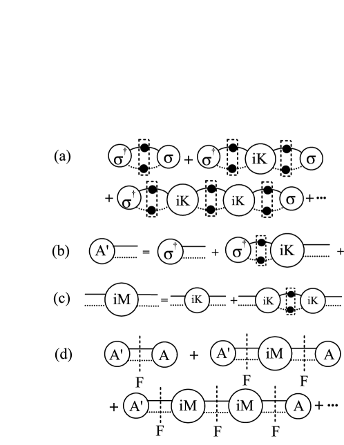
Figure 1: Horizontal dashed lines represent the meson propagators while the solid lines represent the baryon propagators. The corresponding full propagators are represented by dashed/solid lines with a black dot. The dashed rectangles indicate finite volume momentum sum/integrals. Each dashed vertical line indicates an insertion of the factor $F$ entering Eq. (62) which carries the volume dependence of interest. (a) The diagrams that build up the correlation function $C(P)$ defined in Eq. (52); (b) and (c) Diagrams that build up matrix element $A$ and the scattering amplitude $iM$, respectively; (d) The resulting series for the subtracted correlator defined by Eq. (61).

The correlation function $C(P)$ may be built from a series of contributions illustrated by diagrams in FIG. 1(a). In this figure, a solid line with a black dot stands for a full propagator of the baryon while a dashed line with a dot stands for that of the meson. A circle with a symbol $iK$ inside represents the Bethe-Salpeter kernel which consists of all amputated two-particle irreducible diagrams. A circle with a symbol $\sigma$ or $\sigma^{\dagger}$ denotes the interpolating operators in Eq. (52). Using $iK$ we may write the $C(P)$ in the following form:

$$C(P)=\int_{L;q}\sigma_{q}\left[Z_{1}\Delta_{1}Z_{2}\Delta_{2}\right]_{q}\sigma_{q}^{\dagger}$$

$$+ \int_{L;q,q^{\prime}}\sigma_{q}\left[Z_{1}\Delta_{1}Z_{2}\Delta_{2}\right]_{q}iK_{q,q^{\prime}}\left[Z_{1}\Delta_{1}Z_{2}\Delta_{2}\right]_{q^{\prime}}\sigma_{q^{\prime}}^{\dagger}+\cdots$$

where we have adopted the shorthand notation for the two-particle propagators

$$\left[Z_{1}\Delta_{1}Z_{2}\Delta_{2}\right]_{q}=[Z_{1}(q)\Delta_{1}(q)]\cdot[Z_{2}(q)\Delta_{2}(P-q)]\;.$$ (54)

Denoting the interpolating field for the baryon and the meson by $\phi_{1}(x)$ and $\phi_{2}(x)$, respectively, the full propagators appearing in the above equations read

$$Z_{i}(q)\Delta_{i}(q) = \int{d^{4}x}e^{iq\cdot x}\langle\phi_{i}(x)\phi_{i}(0)\rangle\;,\;$$ (55)

$$\Delta_{1}(q) = \frac{i(q^{\mu}\gamma_{\mu}+m_{1})}{q^{2}-m_{1}^{2}+i\varepsilon}\;,$$ (56)

$$\Delta_{2}(q) = \frac{i}{q^{2}-m_{2}^{2}+i\varepsilon}\;.$$ (57)

The factors $Z_{1}(q)$ and $Z_{2}(q)$ are the corresponding dressing functions for the baryon and the meson, respectively. In Eq. (III.1), two-particle intermediate states are summed/integrated in a manner that is appropriate for the finite volume, namely,

$$\int_{L,q}=\frac{1}{L^{3}}\sum_{\mathbf{q}}\int\frac{dq^{0}}{2\pi}\;.$$ (58)

The kernel $iK$ is related to the Bethe-Salpeter kernel $BS$ as

$$iK_{q,q^{\prime}}=iBS(q,P-q,-q^{\prime},-P+q^{\prime})\;,$$ (59)

with $BS$ the sum of all amputated two-particle scattering diagrams which are two-particle-irreducible. Finally the factors $\sigma_{q}$ and $\sigma^{\dagger}_{q}$ denote the coupling of the interpolating operator to the two-particle states.

Normally the interpolating operator is the product of two interpolating operators for the two hadrons being considered, e.g. $\sigma(x)=\phi_{1}(x)\phi_{2}(x)$. In order to have an overlap with the desired states, interpolating operators are usually designed to carry definite $J^{PC}$ quantum numbers. Therefore, without loss of generality, we assume that $\sigma(x)$ carries definite parity. In our case, the operator $\sigma(x)$ must carry Dirac indices as $\phi_{1}(x)$ and since $\gamma_{0}$ is the Dirac matrix responsible for parity transformation for Dirac spinors, we assume that $\sigma(x)$ commute with $\gamma_{0}$. In other words, in what follows, $\gamma_{0}$ may be considered as a $c$-number rather than a matrix in Dirac space.

The kernel $iK$ and the propagator dressing functions $Z_{1,2}(q)$ have only exponentially suppressed dependence on the box size $L$. Such dependence is always assumed to be small and negligible in the large volume limit. The dominant power-law volume dependence enters through the discrete momentum sums in the two-particle loops in Eq. (III.1), the details of these calculations are outlined in appendix B, see Eq. (119). Basically, each summation/integration can be split into two parts:

$$I=I_{\infty}+I_{FV}\;,$$ (60)

where $I_{\infty}$ designates the infinite volume result of the loop integral and $I_{FV}$ contains the finite volume corrections. For each of the loop summations in FIG. 1(a), if we take $I_{\infty}$ in each loop, we then recover the infinite volume correlator $C^{\infty}(P)$. As shown in appendix B, $C^{\infty}(P)$ does not contain the two-particle poles that we are looking for. The part of interest is the finite volume correction:

$$C^{FV}(P)=C(P)-C^{\infty}(P)\;,$$ (61)

where $C^{FV}(P)$ and $C^{\infty}(P)$ are the finite and infinite volume correlation functions, respectively. Diagrammatically, $C^{FV}(P)$ is obtained by keeping at least one insertion of $I_{FV}$ in the two-particle loops in Eq. (III.1). Let $F$ be the kinematic factor associated with the factor of $I_{FV}$. These contributions are shown in Fig. 1(d), leading to the following general result:

$$C^{FV} =-AFA^{\prime}+AF(iM)FA^{\prime}+\ldots$$

$$=-AF\frac{1}{1+iMF}A^{\prime}\;.$$ (62)

The finite volume correction $C^{FV}$ contains the two-particle poles we are looking for.

The factor $F$ is discussed in some detail in appendix B, see Eq. (121). It arises from the integration/summation of the intermediate states represented by the loop diagram, see Eq. (113). Due to the fermion propagator, the factor $F$ is in principle a matrix in Dirac space, as shown in Eq. (114). However, it only contains the matrix $\gamma_{0}$, which is the matrix responsible for the transformation of a Dirac spinor under parity. Since in practical applications we normally choose the interpolating operators $\sigma(x)$ to carry definite parity quantum number, this means that $\gamma_{0}$ can be replaced by its eigenvalues: $\pm 1$. In other words, we can simply treat the function $C(\mathbf{k})$ defined in Eq. (114) as $c$-numbers. Thus, in the COM frame, we simply define:

$$F=C(\mathbf{q}^{\ast})\tilde{F}\;,M=C(\mathbf{q}^{\ast})^{-1}\tilde{M}\;.$$ (63)

with this, Eq. (62) becomes

$$C^{FV} =-AFA^{\prime}+AF(iM)FA^{\prime}+\ldots$$

$$=-AC(\mathbf{q^{\ast}})\tilde{F}A^{\prime}+AC(\mathbf{q^{\ast}})\tilde{F}(i\tilde{M})\tilde{F}A^{\prime}+\ldots$$

$$=-AC(\mathbf{q^{\ast}})\tilde{F}\frac{1}{1+i\tilde{M}\tilde{F}}A^{\prime}\;.$$ (64)

The factors $A$ and $A^{\prime}$ appearing in Eq. (62) may be expressed by appropriate matrix elements of the interpolating operator, as shown in Fig. 1(b). In COM frame the amplitudes $A$ and $A^{\prime}$ now read,

$$\left\{\begin{aligned} A(\mathbf{\hat{k}}^{\ast})&=\langle 0|\sigma(0)|\mathbf{k}^{\ast},-\mathbf{k}^{\ast};\mbox{\rm in}\rangle_{|\mathbf{k}^{\ast}|=q^{\ast}}\\ A^{\prime}(\mathbf{\hat{k}}^{\ast})&=\langle\mathbf{k}^{\ast},-\mathbf{k}^{\ast};\mbox{\rm out}|\sigma^{\dagger}(0)|0\rangle_{|\mathbf{k}^{\ast}|=q^{\ast}}\end{aligned}\right.\;.$$ (65)

Both of these two amplitudes can be viewed as two-component spinor in spin space. It is more useful to express the abstract formula (64) in angular momentum basis. For this purpose, we expand the matrix elements in terms of spin spherical harmonics defined in Eq. (14):

$$\left\{\begin{aligned} A({\mathbf{\hat{k}}^{\ast}})&=\sqrt{4\pi}A_{JMl}Y_{JM}^{l\frac{1}{2}\dagger}(\mathbf{\hat{k}}^{\ast})\\ A^{\prime}(\mathbf{\hat{k}^{\ast}})&=\sqrt{4\pi}A^{\prime}_{JMl}Y_{JM}^{l\frac{1}{2}}(\mathbf{\hat{k}}^{\ast})\end{aligned}\right.\;,$$ (66)

where summation over repeated indices (i.e. $J$, $M$ and $l$) are understood.

Similarly, working in states with definite parity, $\tilde{F}$ and $\tilde{M}$ are viewed as $2\times 2$ matrices in spin space, which can be expanded as well,

$$\tilde{F}(\mathbf{\hat{k}}^{\ast},\mathbf{\hat{k}^{\ast\prime}}) = \frac{-1}{4\pi}\tilde{F}_{JMl;J^{\prime}M^{\prime}l^{\prime}}Y_{JM}^{l\frac{1}{2}}(\mathbf{\hat{k}^{\ast}})Y_{J^{\prime}M^{\prime}}^{l^{\prime}\frac{1}{2}{\dagger}}(\mathbf{\hat{k}^{\ast\prime}})\;,$$ (67)

$$\tilde{M}(\mathbf{\hat{k}}^{\ast},\mathbf{\hat{k}^{\ast\prime}}) = {4\pi}\tilde{M}_{JMl;J^{\prime}M^{\prime}l^{\prime}}Y_{JM}^{l\frac{1}{2}}(\mathbf{\hat{k}^{\ast}})Y_{J^{\prime}M^{\prime}}^{l^{\prime}\frac{1}{2}{\dagger}}(\mathbf{\hat{k}^{\ast\prime}})\;.$$ (68)

Here the notation $Y_{JM}^{l\frac{1}{2}}(\mathbf{\hat{k}^{\ast}})Y_{J^{\prime}M^{\prime}}^{l^{\prime}\frac{1}{2}{\dagger}}(\mathbf{\hat{k}^{\ast\prime}})$ stands for the direct product of two spin spherical harmonics. Then the abstract formula Eq.(64) remains valid except that all implicit indices are in angular momentum space. For example:

$$(AC(\mathbf{q^{\ast}})\tilde{F}\tilde{M}\tilde{F}A^{\prime})_{J_{1}M_{1}l_{1};J_{4}M_{4}l_{4}} = A_{J_{1}M_{1}l_{1}}C(\mathbf{q^{\ast}})\tilde{F}_{J_{1}M_{1}l_{1};J_{2}M_{2}l_{2}}\tilde{M}_{J_{2}M_{2}l_{2};J_{3}M_{3}l_{3}}\tilde{F}_{J_{3}M_{3}l_{3};J_{4}M_{4}l_{4}}A^{\prime}_{J_{4}M_{4}l_{4}}\;,$$ (69)

where the matrix $\tilde{F}_{JMl;J^{\prime}M^{\prime}l^{\prime}}$ is given by:

$$\tilde{F}_{JMl;J^{\prime}M^{\prime}l^{\prime}} =\frac{q^{\ast}}{8\pi{E^{\ast}}}(\delta_{JJ^{\prime}}\delta_{MM^{\prime}}\delta_{ll^{\prime}}+iF_{JMl;J^{\prime}M^{\prime}l^{\prime}}^{FV})$$ (70)

with $\tilde{F}_{JMl;J^{\prime}M^{\prime}l^{\prime}}^{FV}$ given in Eq. (123) in the appendix.

The matrix $\tilde{M}$ in Eq. (64) is the scattering amplitude illustrated in FIG. 1(b) and FIG. 1(c) which can be related to the non-relativistic quantum mechanical scattering matrix $M^{(NR)}$. Following the discussion as in Ref. Lüscher (1991b), the relation is found to be

$$\tilde{M}_{JMl;J^{\prime}M^{\prime}l^{\prime}} = 8\pi{E^{\ast}}M^{(NR)}_{JMl;J^{\prime}M^{\prime}l^{\prime}}\;.$$ (71)

where $M^{(NR)}_{JMl;J^{\prime}M^{\prime}l^{\prime}}$ given by Eq. (92) in appendix A.

The quantization condition can now be obtained for $C^{FV}(P)$ which manifest itself as a series of two-particle poles. This means that the matrix between $A$ and $A^{\prime}$ must have divergent eigenvalues hence satisfy the following condition:

$$\det(1+i\tilde{M}\tilde{F})=0\;.$$ (72)

This is the so-called quantization condition for the two-particle poles in a finite box. In order to compare this with the conventional Lüscher’s formula obtained by non-relativistic approach, we substitute the definitions of $\tilde{M}_{JMl;J^{\prime}M^{\prime}l^{\prime}}$ and $\tilde{F}_{JMl;J^{\prime}M^{\prime}l^{\prime}}$ in Eq. (71) and Eq. (70) into Eq. (72). We then obtain the following result:

$$\det(\tan{\delta_{Jl}}F_{JMl;J^{\prime}M^{\prime}l^{\prime}}^{FV}-\delta_{JJ^{\prime}}\delta_{MM^{\prime}}\delta_{ll^{\prime}}) = 0\;.$$ (73)

Using an equality which will be shown in appendix B, namely Eq. (126), it is seen that $F$ is related to the matrix $\mathcal{M}^{\mathbf{d}}$ up to a possible phase. In the case of strong interaction, the phase factor does not enter, since the Hamiltonian of the system conserves parity and there can be no scattering connecting $l=J+\frac{1}{2}$ with $l=J-\frac{1}{2}$. So the scattering matrix $S^{Jl}=\exp(2i\delta_{Jl})$ must be a diagonal matrix. It is then verified that Eq. (73) reduces to the conventional single-channel Lüscher’s formula in a moving frame discussed in subsection II.2.

III.2 Two-channel case

In this subsection, we generalize the results of a single channel case to the two-channel case. The formalism is the same as in the single channel case except that we need two interpolating operators $\sigma_{j}(x)$ with $j=1,2$ denoting two different channels. In this case, as shown in Fig. 1, the two-point function has the following form,

$$C(P)=\int_{L;q}\sigma_{j;q}[Z_{1}\Delta_{1}Z_{2}\Delta_{2}]_{jg;q}\sigma_{g;q}^{\dagger}+\int_{L;q,q^{\prime}}\sigma_{j;q}[Z_{1}\Delta_{1}Z_{2}\Delta_{2}]_{jg;q}iK_{gh;q,q^{\prime}}[Z_{1}\Delta_{1}Z_{2}\Delta_{2}]_{hr;q^{\prime}}\sigma_{r;q^{\prime}}^{\dagger}+\cdot\cdot\cdot$$ (74)

Here indices $g$, $h$, and $r$ also refer to the channel and take the value $1$ or $2$. In Eq.(74), we have also utilized the following shorthand notations:

$$\left[Z_{1}\Delta_{1}Z_{2}\Delta_{2}\right]_{jg;q}=\delta_{jg}[Z_{j;1}\Delta_{j;1}(q)][Z_{g;2}\Delta_{g;2}(P-q)]\;,$$ (75)

with the definitions

$$Z_{j;I}\Delta_{j;I}(q)=\int{d^{4}x}e^{iq\cdot x}\langle\phi_{j;I}(x)\phi_{j;I}(0)\rangle\;,$$ (76)

$$\Delta_{j;1}(q)=\frac{i(q^{\mu}\gamma_{\mu}+m_{j;1})}{q^{2}-m_{j;1}^{2}+i\varepsilon}\;,$$ (77)

$$\Delta_{j;2}(q)=\frac{i}{q^{2}-m_{j;2}^{2}+i\varepsilon}\;.$$ (78)

So we have two indices for the propagators and their dressing functions: $\Delta_{j;I}$ (and the corresponding mass values $m_{j;I}$ which enters the propagator) and $Z_{j;I}$. The first index $j=1,2$ designates two different scattering channels. The second index $I=1,2$ now denotes particle types: $I=1$ for the baryon and $I=2$ for the meson.

The kernel $K_{gh}$ is again related to the Bethe-Salpeter kernel $BS_{gh}$ which now becomes a matrix in channel space. The matrix elements of interpolating fields $\sigma_{j}$ become vectors in channel space. We have also assumed that $\sigma_{j}$ carry definite parity quantum numbers. So similar to Eq. (65), we have,

$$\left\{\begin{aligned} A_{j}(\mathbf{\hat{k}^{\ast}})&=\langle 0|\sigma_{j}(0)|\mathbf{k}^{\ast},-\mathbf{k}^{\ast};j;\mbox{\rm in}\rangle_{|\mathbf{k}^{\ast}|=q_{j}^{\ast}}\\ A_{j}^{\prime}(\mathbf{\hat{k}^{\ast}})&=\langle\mathbf{k}^{\ast},-\mathbf{k}^{\ast};j;\mbox{\rm out}|\sigma^{\dagger}_{j}(0)|0\rangle_{|\mathbf{k}^{\ast}|=q_{j}^{\ast}}\end{aligned}\right.\;.$$ (79)

In angular momentum basis, expansion (66) becomes

$$\left\{\begin{aligned} A_{j}(\mathbf{\hat{k}^{\ast}})&=\sqrt{4\pi}A_{j;JMl}Y_{JM}^{l\frac{1}{2}{\dagger}}(\mathbf{\hat{k}^{\ast}})\\ A_{j}^{\prime}(\mathbf{\hat{k}^{\ast}})&=\sqrt{4\pi}A^{\prime}_{j;JMl}Y_{JM}^{l\frac{1}{2}}(\mathbf{\hat{k}^{\ast}})\end{aligned}\right.\;.$$ (80)

The factors $\tilde{F}$ and $\tilde{M}$ entering the quantization condition (72) in the previous subsection have both become $2\times 2$ matrices in channel space. We may expand them in terms of spin spherical harmonics, with the coefficients $\tilde{F}$ being diagonal in channel space:

$$\tilde{F}_{ij;JMl;J^{\prime}M^{\prime}l^{\prime}} = \delta_{ij}\tilde{F}_{i;JMl;J^{\prime}M^{\prime}l^{\prime}}\;.$$ (81)

The diagonal element is given by

$$\tilde{F}_{i;JMl;J^{\prime}M^{\prime}l^{\prime}}=\frac{q^{\ast}}{8\pi{E^{\ast}}}(\delta_{JJ^{\prime}}\delta_{MM^{\prime}}\delta_{ll^{\prime}}+iF_{i;JMl;J^{\prime}M^{\prime}l^{\prime}}^{(FV)})\;.$$ (82)

The scattering matrix $M$, however, is not diagonal in channel space. It is still related to the non-relativistic scattering amplitude via,

$$\tilde{M}_{ij;JMl;J^{\prime}M^{\prime}l^{\prime}} = 8\pi{E^{\ast}}M^{(NR)}_{ij;JMl;J^{\prime}M^{\prime}l^{\prime}}\;,$$ (83)

where $M^{(NR)}_{ij;JMl;J^{\prime}M^{\prime}l^{\prime}}$ is defined in Eq. (LABEL:define_multi_M_nr). According to FIG. 11 (d), Eq. (64) still holds except that the quantities involved have all become matrices or vectors in channel space. The poles in $C^{FV}$ still yield the desired quantization condition (72) with the understanding that both $\tilde{M}$ and $\tilde{F}$ have now become $2\times 2$ matrices in channel space.

We are now in a position to write out the quantization condition to a form that is comparable to the conventional multi-channel Lüscher formula obtained in the previous section. For this purpose, we define a matrix $U^{(FV)}_{i}$ using the matrix $F^{(FV)}_{i}$ in Eq. (82),

$$U_{i;JMl;J^{\prime}M^{\prime}l^{\prime}}^{(FV)}=\left(\frac{F_{i}^{(FV)}+i}{F_{i}^{(FV)}-i}\right)_{JMl;J^{\prime}M^{\prime}l^{\prime}}\;.$$ (84)

Now consider an arbitrary moving frame. As we will show in appendix B, see Eq. (128), the matrix element $F^{(FV)}_{i;JMl;J^{\prime}M^{\prime}l^{\prime}}$ is in fact related to the corresponding matrix element $\mathcal{M}^{\mathbf{d}}_{i;JMl;J^{\prime}M^{\prime}l^{\prime}}$ that have appeared in our discussion in subsection II.2, c.f. Eq. (44):

$$F^{(FV)}_{i;JMl;J^{\prime}M^{\prime}l^{\prime}}=i^{l-l^{\prime}}\mathcal{M}^{\mathbf{d}}_{i;JMl;J^{\prime}M^{\prime}l^{\prime}}\;.$$ (85)

This expression is valid up to terms that are exponentially suppressed in the large volume limit. Note that if the Hamiltonian conserves parity such that scattering only occurs for $l=l^{\prime}$, the two matrices become identical. Substituting the definitions of $\tilde{M}_{ij;JMl;J^{\prime}M^{\prime}l^{\prime}}(\ref{field_scattering_amplitude_1})$ and $\tilde{F}_{ij;JMl;J^{\prime}M^{\prime}l^{\prime}}(\ref{field_scattering_F})$ to the quantization condition Eq. (72), we arrive at the following result:

$$\left|\begin{array}[c]{cc}(F_{1;JMl;J^{\prime}M^{\prime}l^{\prime}}^{(FV)}+i)-S_{11}^{Jl}(F_{1;JMl;J^{\prime}M^{\prime}l^{\prime}}^{(FV)}-i)&\sqrt{\frac{q_{2}^{\ast}}{q_{1}^{\ast}}}S_{21}^{Jl}(F_{2;JMl;J^{\prime}M^{\prime}l^{\prime}}^{(FV)}-i)\\ \sqrt{\frac{q_{1}^{\ast}}{q_{2}^{\ast}}}S_{12}^{Jl}(F_{1;JMl;J^{\prime}M^{\prime}l^{\prime}}^{(FV)}-i)&(F_{2;JMl;J^{\prime}M^{\prime}l^{\prime}}^{(FV)}+i)-S_{22}^{Jl}(F_{2;JMl;J^{\prime}M^{\prime}l^{\prime}}^{(FV)}-i)\end{array}\right| = 0\;.$$ (88)

Comparing (33) with (88), we find that the forms of these formulae are completely equivalent although we have used different methods to obtain them. This conclusion is valid up to terms which vanish exponentially with the box size.

IV Discussions and conclusions

In this paper, we have generalized Lüscher’s formula to the case of multi-channel two-particle (one spinless, one spin-$1/2$) scattering in a cubic box. The generalization was done using both non-relativistic quantum mechanics and quantum field theory. We verified that, up to terms that are exponentially suppressed in the large volume limit, both methods yield compatible results.

Although we only consider the case of meson-baryon scattering in this paper, using similar techniques, it should not be too difficult to generalize the results to the case of scattering between hadrons with other spin configurations. In fact, using similar notations as in Refs. Bernard et al. (2008); Ishizuka (2009), one should be able to obtain corresponding formulae suitable for nucleon-nucleon multi-channel scattering. Another interesting direction is the corresponding formulae in a box with different boundary conditions, which turns out to be useful for practical reasons. In particular, the formulae obtained in this paper can readily be generalized for anti-periodic or twisted boundary conditions.

A unique feature of the multi-channel scattering Lüscher’s formula which differs from that in the single-channel case is that, the corresponding equation is not a one-to-one relation between the energy and the corresponding scattering parameters. Therefore, even if one can construct appropriate correlation functions to obtain the two-particle energy $E$ in lattice simulations, Lüscher’s formulae only sets up constraints among the energy $E$ and the $S$-matrix parameters $S^{Jl}_{ij}(E)$. Further physical inputs are needed to really pin down these scattering parameters in a multi-channel scenario.

Finally, let us discuss some possible applications of Lüscher’s formula in multi-channel scattering. One typical example is the antikaon-nucleon scattering. The scattering amplitude of antikaon-nucleon is of fundamental importance in the study of $\Lambda$(1405) resonance which just exceeds the scattering threshold. There is a strong coupling between $\bar{K}$N and $\Sigma\pi$ channels when the energy exceeds $\bar{K}$N threshold. It becomes a problem for two-particle scattering, one with spin $\frac{1}{2}$ and one with spin $0$ in two channels. In Ref. Lage et al. (2009b), the authors used two channel Lippmann-Schwinger equation to study the problem. In Ref. Martinez Torres et al. (2012), the same problem was addressed using unitarized chiral perturbation theory. In principle, this problem can also be studied using Lüscher’s formula in lattice QCD simulations, although that requires more data than we currently can acquire. Another example is the $DN$ and $\pi\Sigma_{c}$ coupled channels scattering studied in Ref. Xie and Oset (2012).

To summarize, in this paper we generalize Lüscher’s formula to the case of particles with spin, beyond the inelastic threshold in COM frame and MF respectively. Using a quantum mechanical model and quantum field theory, a relation between the energy of the two-particle system and scattering matrix elements is found. It is verified that the two methods yields the same result if we neglect terms that are exponentially suppressed in the large volume limit. Although we focus on the case of scattering between two particles: one with spin $0$ and the other with spin $\frac{1}{2}$, we do not see any essential difficulties to generalize the situation to any spin with any number of channels. We hope that these relations will help us to study multi-channel hadron scattering between particles with spin using lattice QCD in the future.

Appendix A Single-channel spin-dependent scattering

In this appendix, we first briefly review single channel scattering of a particle with spin in quantum mechanics in infinite volume. After that, single channel Lüscher’s formulae are collected which can be found in Refs. Bernard et al. (2008); Ishizuka (2009); Rummukainen and Gottlieb (1995); Fu (2012). Similar formulae in the multi-channel case are listed afterwards at the end of this appendix.

To avoid inessential complications, we shall only discuss the case of two stable particles with spin $0$ and spin $\frac{1}{2}$ in COM frame. In non-relativistic quantum mechanics, after factoring out the center of mass motions, the asymptotic form of the wave function is:

$$\psi_{s}(\mathbf{r})=\chi^{\frac{1}{2}}_{s}e^{i\mathbf{k\cdot{r}}}+\sum_{s^{\prime}}\chi^{\frac{1}{2}}_{s^{\prime}}M^{(NR)}_{s^{\prime}s}(\mathbf{\hat{k}\cdot\hat{r}})\frac{e^{ikr}}{r}\;.$$ (89)

This form has the property that, in the remote past, it reduces to an incident plane wave with prescribed quantum numbers (linear momentum and spin). In Ref. Newton (1982), the scattering amplitude between particles with spin 0 and spin $\frac{1}{2}$ is given by,

$$M^{(NR)}_{s^{\prime}s}(\mathbf{\hat{k}\cdot{\hat{r}}}) = \frac{4\pi}{2ik}\sum_{l=0}^{\infty}\sum_{J=l-\frac{1}{2}}^{l+\frac{1}{2}}\sum_{M=-J}^{J}(S^{Jl}-1)\mathfrak{Y}_{JMls^{\prime}}(\mathbf{\hat{r}})\mathfrak{Y}_{JMls}^{\ast}(\mathbf{\hat{k}})\;,$$ (90)

where the auxiliary spin spherical harmonic function $\mathfrak{Y}_{JMls}(\mathbf{\hat{r}})$ in spin-space is defined as

$$\mathfrak{Y}_{JMls}(\mathbf{\hat{r}})=i^{-l}\chi^{\frac{1}{2}\dagger}_{s}\cdot{Y^{l\frac{1}{2}}_{JM}(\mathbf{\hat{r}})}\;.$$ (91)

The dot here indicates an inner product in spin space. This means that the scattering matrix is diagonal in angular-momentum basis:

$$M^{(NR)}_{JMl;J^{\prime}M^{\prime}l^{\prime}} = M^{(NR)}_{J^{\prime}M^{\prime}l^{\prime};JMl}$$ (92)

$$= \delta_{J^{\prime}J}\delta_{M^{\prime}M}\delta_{l^{\prime}l}\frac{1}{2ik}(S^{Jl}-1)\;.$$

For single channel spin-dependent scattering, the $S$-matrix is parameterized by $S^{Jl}=e^{2i\delta_{Jl}}$. Since $J$ can take two possible values, $J=l\pm 1/2$, we will also conveniently denote them as $S^{J=l\pm 1/2,l}=S^{l\pm}=\exp(2i\delta_{l\pm})$.

If we have chosen the $z$-axis to coincide with the incident momentum $\mathbf{\hat{k}}$, the scattering amplitude depends only on $\theta$:

$$M^{(NR)}_{s^{\prime}s}(\theta) = \frac{1}{2ik}\sum_{l=0}^{\infty}\sum_{J=l-\frac{1}{2}}^{l+\frac{1}{2}}\sqrt{4\pi(2l+1)}(S^{Jl}-1)S^{l\frac{1}{2}}_{JM;ms^{\prime}}S^{l\frac{1}{2}}_{JM;0s}Y_{lm}(\mathbf{\hat{r}})\;.$$ (93)

Due to the Clebsch-Gordan coefficients $S^{l\frac{1}{2}}_{JM;0s}$ and $S^{l\frac{1}{2}}_{JM;ms^{\prime}}$, we find: $M=s$ and $m=M-s^{\prime}$. Thus, in the previous equation we ignore the sum over $M$ and $m$ for a given pair of $s$ and $s^{\prime}$. It is then clear that $M(\theta)$ as a matrix in spin space can also be written in the following form

$$M(\theta)=f(\theta)+ig(\theta)({\mbox{\boldmath$\sigma$}}\cdot\mathbf{e})\;,$$ (94)

where $f(\theta)$ and $g(\theta)$ are known as no-flip and spin-flip amplitudes, respectively. $\sigma$ is the Pauli matrices in spin space and $\mathbf{e}$ is a unit vector perpendicular to the scattering plane. With this convention, these functions are given by

$$\left\{\begin{aligned} f(\theta)&=\sum_{l=0}^{\infty}[(l+1)f_{l+}+lf_{l-}]P_{l}(\cos\theta)\\ g(\theta)&=\sum_{l=0}^{\infty}[f_{l+}-f_{l-}]P^{1}_{l}(\cos\theta)\end{aligned}\right.\;.$$ (95)

with $f_{l\pm}(k)=e^{i\delta_{l\pm}}\sin(\delta_{l\pm})/k$. These are identical to what have appeared in the early literature, see for example, Ref. Hamilton and Woolcock (1963) and Ref. Chew et al. (1957).

Let us now enclose the system we considered in a large cubic box with periodic boundary conditions applied in all three spatial directions. The interaction is only present in the inner region while in the outer region, the radial wave function becomes a superposition of $n_{l}(kr)$ and $j_{l}(kr)$,

$$\psi(\mathbf{r})=\sum_{JMl}(\alpha_{Jl}(k)j_{l}(kr)+\beta_{Jl}(k)n_{l}(kr))Y_{JM}^{l\frac{1}{2}}(\mathbf{\hat{r}})$$ (96)

which leads to the identification $\tan(\delta_{Jl}(k))=\beta_{Jl}(k)/\alpha_{Jl}(k)$. The Green’s functions, which are singular periodic solutions of the Helmholtz equation, has a similar expansion. In this case, it is similar to those introduced in Ref. Lüscher (1991a) (see also e.g. Ref. Bernard et al. (2008); Ishizuka (2009)):

$$G_{JMl}(\textbf{r},k^{2})=\frac{(-1)^{l}k^{l+1}}{4\pi}\left(Y_{JM}^{l\frac{1}{2}}(\mathbf{{\hat{r}}})n_{l}(kr)+\underset{J^{\prime}M^{\prime}l^{\prime}}{\sum}\mathcal{M}_{JMl;J^{\prime}M^{\prime}l^{\prime}}(k^{2})Y_{J^{\prime}M^{\prime}}^{l^{\prime}\frac{1}{2}}(\mathbf{{\hat{r}}})j_{l^{\prime}}(kr)\right)\;.$$ (97)

Comparing Eq. (96) with Eq. (97) and following similar steps as in the derivation of the conventional Lüscher’s formula, one finally finds

$$\det[\tan\delta_{Jl}(k)\mathcal{M}_{JMl;J^{\prime}M^{\prime}l^{\prime}}-\delta_{JJ^{\prime}}\delta_{MM^{\prime}}\delta_{ll^{\prime}}]=0$$ (98)

which is the same as in Ref. Bernard et al. (2008). The explicit form of $\mathcal{M}_{JMl;J^{\prime}M^{\prime}l^{\prime}}$ is given in Ref. Bernard et al. (2008) which we quote here:

$$\mathcal{M}_{JMl;J^{\prime}M^{\prime}l^{\prime}} = \sum_{mm^{\prime}s}\mathcal{M}_{lm;l^{\prime}m^{\prime}}\langle{lm\frac{1}{2}s}|JM\rangle\langle{l^{\prime}m^{\prime}\frac{1}{2}s}|J^{\prime}M^{\prime}\rangle\;,$$ (99)

$$\mathcal{M}_{lm;l^{\prime}m^{\prime}} = \frac{(-1)^{l}}{\pi^{\frac{3}{2}}}\sum_{t=|l-l^{\prime}|}^{l+l^{\prime}}\sum^{t}_{n=-t}\frac{i^{t}}{\boldsymbol{\kappa}^{t+1}}Z_{tn}(1;\boldsymbol{\kappa}^{2})C_{lm,tn,l^{\prime}m^{\prime}}$$ (100)

with $\boldsymbol{\kappa}=\mathbf{k}L/(2\pi)$ and the zeta function $Z_{tn}(1;\boldsymbol{\kappa}^{2})$ and the coefficients $C_{lm,tn,l^{\prime}m^{\prime}}$ are given respectively by

$$Z_{tn}(1;\boldsymbol{\kappa}^{2}) = \sum_{\mathbf{n}\in{\mathbbm{Z}^{3}}}\frac{|\mathbf{n}|^{t}Y_{tn}(\mathbf{\hat{n}})}{\mathbf{n}^{2}-\boldsymbol{\kappa}^{2}}\;,$$ (101)

$$C_{lm,tn,l^{\prime}m^{\prime}} = i^{l-t+l^{\prime}}\sqrt{\frac{(2l+1)(2t+1)}{(2l^{\prime}+1)}}\langle{l0t0}|l^{\prime}0\rangle\langle{lmtn}|l^{\prime}m^{\prime}\rangle\;.$$ (102)

The corresponding formulae in moving frames have been obtained in Ref. Rummukainen and Gottlieb (1995); Fu (2012). For example, instead of Eq. (99), we have,

$$\mathcal{M}^{\mathbf{d}}_{lm;l^{\prime}m^{\prime}}=\frac{(-1)^{l}}{\gamma\pi^{\frac{3}{2}}}\sum_{t,n}\frac{i^{t}}{\boldsymbol{\kappa}^{t+1}}Z^{\mathbf{d}}_{tn}(1;\boldsymbol{\kappa}^{2}){C_{lm,tn,l^{\prime}m^{\prime}}}$$ (103)

with $\boldsymbol{\kappa}=\mathbf{k}L/(2\pi)$, the parameter $\gamma$ is the Lorentz boost factor associated with the moving-frame and the zeta function $Z^{\mathbf{d}}_{tn}(1;\boldsymbol{\kappa}^{2})$ is defined by

$$Z^{\mathbf{d}}_{tn}(1;\boldsymbol{\kappa}^{2}) = \sum_{\mathbf{n}\in\mathcal{P}_{\mathbf{d}}}\frac{|\mathbf{n}|^{t}Y_{tn}(\mathbf{\hat{n}})}{\mathbf{n}^{2}-\boldsymbol{\kappa}^{2}}\;,$$ (104)

the coefficients $C_{lm,tn,l^{\prime}m^{\prime}}$ are the same as in non-moving frames, e.g. Eq. (101). In the above formulae,

$$\mathcal{P}_{\mathbf{d}}=\left\{\mathbf{r}\left|\mathbf{r}=\vec{\gamma}^{-1}(\mathbf{n}+\frac{1}{2}\alpha{\mathbf{d}})\;\;\;\mathbf{n}\in{\mathbbm{Z}^{3}}\right.\right\}\;,$$ (105)

where $\alpha$ and $\mathbf{d}$ are given as in subsection II.2. Then Eq. (99) still holds except that one has to use the moving-frame versions ($\mathcal{M}^{\mathbf{d}}_{JMl;J^{\prime}M^{\prime}l^{\prime}}$ and $\mathcal{M}^{\mathbf{d}}_{lm;l^{\prime}m^{\prime}}$) in place of the non-moving frame versions.

Extension of the above formulae to the case of multi-channel case is straightforward. For example, Eq. (92) is generalized to

$$M^{(NR)}_{ij;JMl;J^{\prime}M^{\prime}l^{\prime}} = M^{(NR)}_{ij;J^{\prime}M^{\prime}l^{\prime};JMl}$$

$$= \delta_{J^{\prime}J}\delta_{M^{\prime}M}\delta_{l^{\prime}l}\frac{1}{2i\sqrt{k_{i}k_{j}}}(S_{ij}^{Jl}-\delta_{ij})\;.$$

Similarly, Eq. (99) is modified to:

$$\mathcal{M}^{\mathbf{d}}_{i;JMl;J^{\prime}M^{\prime}l^{\prime}}=\sum_{mm^{\prime}s}\mathcal{M}^{\mathbf{d}}_{i;lm;l^{\prime}m^{\prime}}\langle{lm\frac{1}{2}s}|JM\rangle\langle{l^{\prime}m^{\prime}\frac{1}{2}s}|J^{\prime}M^{\prime}\rangle$$ (107)

with $\mathcal{M}^{\mathbf{d}}_{i;lm;l^{\prime}m^{\prime}}$ given in terms of the zeta function $Z^{\mathbf{d}}_{i;tn}(1;\boldsymbol{\kappa_{i}}^{2})$ like Eq. (103), with $\boldsymbol{\kappa}_{i}=\mathbf{k_{i}}L/(2\pi)$.

Appendix B Calculation the the kinematic factor of loop integration/summation in a single channel

In this appendix, we use the notation: $k^{\ast}=|\mathbf{k^{\ast}}|$, $q^{\ast}=|\mathbf{q^{\ast}}|$ unless otherwise stated.

The generic finite-volume corrections that we are interested in has the following form:

$$S(\mathbf{q^{\ast}}) = \frac{1}{L^{3}}\sum_{\mathbf{k}}\frac{w_{\mathbf{k}}^{\ast}}{w_{\mathbf{k}}}\frac{f^{\ast}(\mathbf{k}^{\ast})}{q^{{\ast}2}-k^{{\ast}2}}\;,$$ (108)

where the function $f^{\ast}(\mathbf{k}^{\ast})$ has no singularities for real $\mathbf{k}^{\ast}$ and falls off fast enough at $k^{\ast}\rightarrow\infty$ so as to render the summation convergent. To simplify the matter, we assume that it is spin-independent and thus can be expanded into spherical harmonics as in Ref. Kim et al. (2005):

$$f^{\ast}(\mathbf{k}^{\ast})=\sum_{l=0}^{\infty}\sum_{m=-l}^{l}f^{\ast}_{lm}(k^{\ast})k^{{\ast}l}\sqrt{4\pi}Y_{lm}(\mathbf{\hat{k}}^{\ast})\;.$$ (109)

One would like to study the behavior of $S(\mathbf{q^{\ast}})$ in the limit of large $L$. For a fixed $L$, if there is no term in the sum with $k^{{\ast}2}\simeq q^{{\ast}2}$, we can replace the sum by an integration. The singularity at $k^{{\ast}2}\simeq q^{{\ast}2}$ for large $L$ forbids this simple replacement. Basically $S(\mathbf{q^{\ast}})$ will split into two parts, one of which can be approximated by the principle-valued integral, the other being the finite volume correction. This has been established in Ref. Kim et al. (2005) and we directly quote their final results:

$$S(\mathbf{q^{\ast}}) = \mathcal{P}\int\frac{d^{3}k^{\ast}}{(2\pi)^{3}}\frac{f^{\ast}(\mathbf{k}^{\ast})}{q^{{\ast}2}-k^{{\ast}2}}+\sum_{l,m}f_{lm}C^{P}_{lm}(q^{*2})\;,$$

$$C^{P}_{lm}(q^{{\ast}2}) = \frac{1}{L^{3}}\sum_{\mathbf{k}}\frac{w_{\mathbf{k}}^{\ast}}{w_{\mathbf{k}}}\frac{e^{\alpha(q^{{\ast}2}-k^{{\ast}2})}}{q^{{\ast}2}-k^{{\ast}2}}k^{{\ast}l}\sqrt{4\pi}Y_{lm}(\mathbf{\hat{k}}^{\ast})$$ (111)

$$-\mathcal{P}\int\frac{d^{3}k^{\ast}}{(2\pi)^{3}}\frac{e^{\alpha(q^{{\ast}2}-k^{{\ast}2})}}{q^{{\ast}2}-k^{{\ast}2}}\;,$$

where $\mathcal{P}$ stands for the principal-value prescription. This summation formula will be utilized shortly.

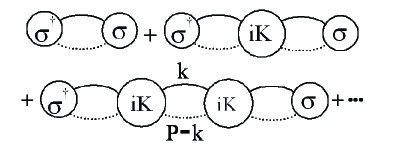
Figure 2: The dash line represents the meson propagator, and the solid line represents the baryon propagator. A circle with a symbol $iK$ inside stands for the Bethe-Salpeter kernel which consists of all amputated two-particle irreducible diagrams. A circle with a symbol $\sigma$ or $\sigma^{\dagger}$ denotes the interpolating operators in Eq. 52.

We now come to the correlation function $C(P)$ defined in Eq(52). It can be expressed in terms of the Bethe-Salpeter kernel $iK$ through the series shown in Fig. 2. The loop integration/summation appearing in the figure has the following form:

$$I=\frac{-1}{L^{3}}\sum_{\mathbf{{k}}}\int\frac{dk_{0}}{2\pi}\frac{f(k_{0},\mathbf{k})(k^{\mu}\gamma_{\mu}+m_{1})}{(k^{2}-m_{1}^{2}+i\varepsilon)((P-k)^{2}-m_{2}^{2}+i\varepsilon)}\;,$$ (112)

where $k=(k_{0},\mathbf{k})$, $P=(E,\mathbf{P})$ being the corresponding four-momenta and $m_{1}$ and $m_{2}$ being the masses of the baryon and the meson respectively. The function $f(k)$ contains the energy-momentum dependence arising from the kernels as well as that from the dressed propagators. The properties of $f(k)$ is such that there exists no singularities for real $\mathbf{k}$ and its ultraviolet behavior is to render the integration or summation convergent. Integrating out $k_{0}$ one gets

$$I=\frac{-i}{L^{3}}\sum_{\mathbf{k}}\left(\frac{f(w_{1\mathbf{k}},\mathbf{k})C(\mathbf{k})}{2w_{1\mathbf{k}}((E-w_{1\mathbf{k}})^{2}-w_{2\mathbf{k}}^{2})}+\frac{f(E+w_{2\mathbf{k}},\mathbf{k})D(\mathbf{k})}{2w_{2\mathbf{k}}((E+w_{2\mathbf{k}})^{2}-w_{1\mathbf{k}}^{2})}\right)\;.$$ (113)

If we assume $f(\mathbf{k})$ is an even function for $\mathbf{k}$

$$\left\{\begin{aligned} C(\mathbf{k})&=(k^{0}\gamma_{0}+m_{1})|_{k_{0}=w_{1\mathbf{k}}}\\ D(\mathbf{k})&=(k^{0}\gamma_{0}+m_{1})|_{k_{0}=E+w_{2\mathbf{k}}}\end{aligned}\right.\;,$$ (114)

and $w_{1\mathbf{k}}=\sqrt{\mathbf{k}^{2}+m_{1}^{2}}$, $w_{2\mathbf{k}}=\sqrt{(\mathbf{P}-\mathbf{k})^{2}+m_{2}^{2}}$ are the two energies. Note that both $C(\mathbf{k})$ and $D(\mathbf{k})$ and thus the integral $I$ are matrices in Dirac space. However, as mentioned in the main text, normally the interpolating operators that we formed to create the meson and baryon carry definite parity. This means that, for practical applications, $\gamma_{0}$ takes its eigenvalues, $\pm 1$ times a unit matrix (in spin space). Thus the integral $I$ is written into two parts $I_{1}$ and $I_{2}$ corresponding to the two terms in Eq(113). The second term $I_{2}$ does not contain the finite-volume singularities in the kinematic region of interest and therefore can be replaced by the corresponding integral in the large volume limit. The term which does contain the two-particle finite-volume poles is $I_{1}$,

$$I_{1}=\frac{-i}{L^{3}}\sum_{\mathbf{k}}\frac{f(w_{1\mathbf{k}},\mathbf{k})C(\mathbf{k})}{2w_{1\mathbf{k}}((E-w_{1\mathbf{k}})^{2}-w_{2\mathbf{k}}^{2})}\;.$$ (115)

It is seen that the two-particle pole singularity in $I_{1}$ is located at $E=w_{1\mathbf{k}}+w_{2\mathbf{k}}$. To determine the finite volume correction in more detail, we express the term $I_{1}$ in another form by transforming it in to the COM frame. In COM frame the two energies are: $w^{\ast}_{1\mathbf{k}}=\sqrt{\mathbf{k}^{{\ast}2}+m_{1}^{2}}$, $w^{\ast}_{2\mathbf{k}}=\sqrt{\mathbf{k}^{{\ast}2}+m_{2}^{2}}$ as given in section II.2.Thus we obtain:

$$I_{1} =-\frac{i}{L^{3}}\sum_{\mathbf{k}}\frac{f^{\ast}(\mathbf{k}^{\ast})C(\mathbf{k}^{\ast})}{2w_{1\mathbf{k}}((E^{\ast}-w_{1\mathbf{k}}^{\ast})^{2}-w_{2\mathbf{k}}^{\ast 2})}$$

$$=\frac{-i}{2L^{3}}\sum_{\mathbf{k}}\frac{w_{1\mathbf{k}}^{\ast}}{w_{1\mathbf{k}}}\frac{f^{\ast}(\mathbf{k}^{\ast})C(\mathbf{k}^{\ast})}{q^{\ast 2}-k^{\ast 2}}\left[\frac{(E^{\ast}+w_{1\mathbf{k}}^{\ast})^{2}-w_{2\mathbf{k}}^{\ast 2}}{4E^{\ast 2}w_{1\mathbf{k}}^{\ast}}\right]\;.$$ (116)

By using the summation formula Eq. (B) we mentioned at the beginning of this appendix, we obtain:

$$I_{1} = (-i)\mathcal{P}\int\frac{d^{3}k^{\ast}}{(2\pi)^{3}}\frac{f^{\ast}(\mathbf{k}^{\ast})C(\mathbf{k}^{\ast})}{q^{\ast 2}-k^{\ast 2}}\left[\frac{(E^{\ast}+w_{1\mathbf{k}}^{\ast})^{2}-w_{2\mathbf{k}}^{\ast 2}}{8E^{\ast 2}w_{1\mathbf{k}}^{\ast}}\right]-\frac{iC(\mathbf{q^{\ast}})}{2E^{\ast}}\sum_{lm}f_{lm}^{\ast}(q^{\ast})C_{lm}^{P}(q^{\ast 2})\;.$$ (117)

In order to write $I_{1}$ as the infinite-volume result together with a correction, we replace the principle-value integration in the above formula by a Feynman $+i\varepsilon$ prescription in the propagator and a “delta-function” term which picks out the $l=0$ part of $f^{\ast}$.

$$I_{1} =-i\frac{1}{2E^{\ast}}\int\frac{d^{3}k^{\ast}}{(2\pi)^{3}}\frac{f^{\ast}(\mathbf{k}^{\ast})C(\mathbf{k}^{\ast})}{q^{\ast 2}-k^{\ast 2}+i\varepsilon}\frac{(E^{\ast}+w_{1\mathbf{k}}^{\ast})^{2}-w_{2\mathbf{k}}^{\ast 2}}{4E^{\ast}w_{1\mathbf{k}}^{\ast}}+\frac{q^{\ast}f_{00}^{\ast}(q^{\ast})C(\mathbf{q^{\ast}})}{8\pi{E^{\ast}}}-\frac{iC(\mathbf{q^{\ast}})}{2E^{\ast}}\sum_{lm}f_{lm}^{\ast}(q^{\ast})C_{lm}^{P}(q^{\ast 2})\;.$$ (118)

Finally, we arrive at our final result for $I$,

$$I = I_{\infty}+I_{FV}\;,$$ (119)

where $I_{\infty}$ is the infinite volume result for the original loop integral with the appropriate Feynman’s prescription, $I_{\infty}=I_{1,\infty}+I_{2}$. As mentioned earlier, $I_{\infty}$ contains no finite volume singularities. The two-particle singularities are contained in the finite volume correction term, $I_{FV}$ which is given by

$$I_{FV} = \frac{q^{\ast}f_{00}^{\ast}(q^{\ast})C(\mathbf{q^{\ast}})}{8\pi{E^{\ast}}}-\frac{iC(\mathbf{q^{\ast}})}{2E^{\ast}}\sum_{lm}f_{lm}^{\ast}(q^{\ast})C_{lm}^{P}(q^{\ast 2})\;.$$

Using the expansion (109) and the completeness of spherical harmonics, we obtain,

$$F \equiv C(\mathbf{q^{\ast}})\tilde{F}=\frac{q^{\ast}C(\mathbf{q^{\ast}})}{8\pi{E^{\ast}}}(1+iF^{FV})\;,$$ (121)

$$\tilde{F}_{JMl;J^{\prime}M^{\prime}l^{\prime}} = \frac{q^{\ast}}{8\pi{E^{\ast}}}(\delta_{JJ^{\prime}}\delta_{MM^{\prime}}\delta_{ll^{\prime}}+iF_{JMl;J^{\prime}M^{\prime}l^{\prime}}^{FV})\;,$$ (122)

$$F_{JMl;J^{\prime}M^{\prime}l^{\prime}}^{FV} = \frac{-4\pi}{q^{\ast}}\sum_{l_{1}m_{1}}\frac{\sqrt{4\pi}}{q^{\ast l_{1}}}{C_{l_{1}m_{1}}^{P}}\int{d\Omega^{\ast}}Y_{JM}^{l\frac{1}{2}\dagger}Y_{l_{1}m_{1}}^{\ast}Y_{J^{\prime}M^{\prime}}^{l^{\prime}\frac{1}{2}}\;,$$ (123)

$$C^{P}_{l_{1}m_{1}}(q^{{\ast}2}) = \frac{1}{L^{3}}\sum_{\mathbf{k}}\frac{w_{1\mathbf{k}}^{\ast}}{w_{1\mathbf{k}}}\frac{e^{\alpha(q^{{\ast}2}-k^{{\ast}2})}}{q^{{\ast}2}-k^{{\ast}2}}k^{{\ast}l_{1}}\sqrt{4\pi}Y_{l_{1}m_{1}}-\mathcal{P}\int\frac{d^{3}k^{\ast}}{(2\pi)^{3}}\frac{e^{\alpha(q^{{\ast}2}-k^{{\ast}2})}}{q^{{\ast}2}-k^{{\ast}2}}\;,$$ (124)

where $\mathcal{P}$ stands for the principal-value prescription.

In Ref. Briceno and Davoudi (2012), for the scattering of two particles with different masses, a relation between $C^{P}_{lm}(q^{{\ast}2})$ and $Z^{\mathbf{d}}_{lm}(1;\boldsymbol{\kappa}^{2})$ is found,

$$C^{P}_{lm}(q^{{\ast}2})=-\frac{\sqrt{4\pi}}{\gamma{L^{3}}}(\frac{2\pi}{L})^{l-2}Z^{\mathbf{d}}_{lm}(1;\boldsymbol{\kappa}^{2})$$ (125)

with $\boldsymbol{\kappa}=\mathbf{q^{\ast}}L/(2\pi)$, $Z^{\mathbf{d}}_{lm}(1;\boldsymbol{\kappa}^{2})$ is defined by (104). This equality holds up to terms which vanish exponentially with the box size. Thus, according to the expressions for $F^{FV}_{JMl;J^{\prime}M^{\prime}l^{\prime}}$ and $\mathcal{M}^{\mathbf{d}}_{JMl;J^{\prime}M^{\prime}l^{\prime}}$ i.e. Eq. (123) and Eq. (107) we have the following equality:

$$F^{FV}_{JMl;J^{\prime}M^{\prime}l^{\prime}} = i^{l-l^{\prime}}\mathcal{M}^{\mathbf{d}}_{JMl;J^{\prime}M^{\prime}l^{\prime}}$$ (126)

which is also valid up to terms that vanish exponentially with the box size. In the case of multi-channel scattering, the above formulae is naturally modified to:

$$C^{P}_{i;lm}(q_{i}^{\ast 2})=-\frac{\sqrt{4\pi}}{\gamma{L^{3}}}(\frac{2\pi}{L})^{l-2}Z^{\mathbf{d}}_{i;lm}(1;\boldsymbol{\kappa}_{i}^{2})$$ (127)

with $\boldsymbol{\kappa}_{i}=\mathbf{q_{i}^{\ast}}L/(2\pi)$ and Eq. (126) is modified to

$$F^{FV}_{i;JMl;J^{\prime}M^{\prime}l^{\prime}} = i^{l-l^{\prime}}\mathcal{M}^{\mathbf{d}}_{i;JMl;J^{\prime}M^{\prime}l^{\prime}}\;.$$ (128)

Again, these formulae hold up to terms that are vanishing exponentially in the box size. These equalities are utilized when we compare Lüscher’s formulae obtained from quantum field theory with those obtained from non-relativistic quantum mechanics.

References

- Hansen and Sharpe (2012) M. T. Hansen and S. R. Sharpe, (2012), arXiv:1204.0826 [hep-lat] .
- Lüscher (1986) M. Lüscher, Comm. Math. Phys. 105, 153 (1986).
- Lüscher and Wolff (1990) M. Lüscher and U. Wolff, Nucl. Phys. B 339, 222 (1990).
- Lüscher (1991a) M. Lüscher, Nucl. Phys. B 354, 531 (1991a).
- Lüscher (1991b) M. Lüscher, Nucl. Phys. B 364, 237 (1991b).
- Gockeler et al. (1994) M. Gockeler, H. A. Kastrup, J. Westphalen, and F. Zimmermann, Nucl.Phys. B425, 413 (1994), arXiv:hep-lat/9402011 [hep-lat] .
- Gupta et al. (1993) R. Gupta, A. Patel, and S. R. Sharpe, Phys.Rev. D48, 388 (1993), arXiv:hep-lat/9301016 [hep-lat] .
- Fukugita et al. (1995) M. Fukugita, Y. Kuramashi, M. Okawa, H. Mino, and A. Ukawa, Phys.Rev. D52, 3003 (1995), arXiv:hep-lat/9501024 [hep-lat] .
- Aoki et al. (2000) S. Aoki et al. (JLQCD Collaboration), Nucl.Phys.Proc.Suppl. 83, 241 (2000), arXiv:hep-lat/9911025 [hep-lat] .
- Aoki et al. (2002) S. Aoki et al. (JLQCD Collaboration), Phys.Rev. D66, 077501 (2002), arXiv:hep-lat/0206011 [hep-lat] .
- Liu et al. (2002) C. Liu, J.-h. Zhang, Y. Chen, and J. Ma, Nucl.Phys. B624, 360 (2002), arXiv:hep-lat/0109020 [hep-lat] .
- Hasenfratz et al. (2004) P. Hasenfratz, K. Juge, and F. Niedermayer (Bern-Graz-Regensburg Collaboration), JHEP 0412, 030 (2004), arXiv:hep-lat/0411034 [hep-lat] .
- Du et al. (2004) X. Du, G.-w. Meng, C. Miao, and C. Liu, Int.J.Mod.Phys. A19, 5609 (2004), arXiv:hep-lat/0404017 [hep-lat] .
- Aoki et al. (2005) S. Aoki et al. (CP-PACS Collaboration), Phys.Rev. D71, 094504 (2005), arXiv:hep-lat/0503025 [hep-lat] .
- Aoki et al. (2003) S. Aoki et al. (CP-PACS Collaboration), Phys.Rev. D67, 014502 (2003), arXiv:hep-lat/0209124 [hep-lat] .
- Yamazaki et al. (2004) T. Yamazaki et al. (CP-PACS Collaboration), Phys.Rev. D70, 074513 (2004), arXiv:hep-lat/0402025 [hep-lat] .
- Beane et al. (2006a) S. R. Beane, P. F. Bedaque, K. Orginos, and M. J. Savage (NPLQCD Collaboration), Phys.Rev. D73, 054503 (2006a), arXiv:hep-lat/0506013 [hep-lat] .
- Li and Liu (2004) X. Li and C. Liu, Phys. Lett. B587, 100 (2004), arXiv:hep-lat/0311035 .
- Feng et al. (2004) X. Feng, X. Li, and C. Liu, Phys. Rev. D70, 014505 (2004), arXiv:hep-lat/0404001 .
- Li et al. (2007) X. Li et al. (CLQCD), JHEP 06, 053 (2007), arXiv:hep-lat/0703015 .
- Rummukainen and Gottlieb (1995) K. Rummukainen and S. A. Gottlieb, Nucl.Phys. B450, 397 (1995), arXiv:hep-lat/9503028 [hep-lat] .
- Xu Feng (2011) D. B. R. Xu Feng, Karl Jansen, (2011), arXiv:1104.0058 [hep-lat] .
- Davoudi and Savage (2011) Z. Davoudi and M. J. Savage, Phys.Rev. D84, 114502 (2011), arXiv:1108.5371 [hep-lat] .
- Fu (2012) Z. Fu, Phys.Rev. D85, 074501 (2012), arXiv:1110.1422 [hep-lat] .
- Gockeler et al. (2012) M. Gockeler, R. Horsley, M. Lage, U.-G. Meissner, P. Rakow, et al., (2012), arXiv:1206.4141 [hep-lat] .
- Bedaque and Chen (2005) P. F. Bedaque and J.-W. Chen, Phys.Lett. B616, 208 (2005), arXiv:hep-lat/0412023 [hep-lat] .
- Bedaque (2004) P. F. Bedaque, Phys.Lett. B593, 82 (2004), arXiv:nucl-th/0402051 [nucl-th] .
- Sachrajda and Villadoro (2005) C. Sachrajda and G. Villadoro, Phys.Lett. B609, 73 (2005), arXiv:hep-lat/0411033 [hep-lat] .
- de Divitiis et al. (2004) G. de Divitiis, R. Petronzio, and N. Tantalo, Phys.Lett. B595, 408 (2004), arXiv:hep-lat/0405002 [hep-lat] .
- Beane et al. (2006b) S. Beane, P. Bedaque, K. Orginos, and M. Savage, Phys.Rev.Lett. 97, 012001 (2006b), arXiv:hep-lat/0602010 [hep-lat] .
- Beane et al. (2004) S. Beane, P. Bedaque, A. Parreno, and M. Savage, Phys.Lett. B585, 106 (2004), arXiv:hep-lat/0312004 [hep-lat] .
- Meng et al. (2004) G.-w. Meng, C. Miao, X.-n. Du, and C. Liu, Int.J.Mod.Phys. A19, 4401 (2004), arXiv:hep-lat/0309048 [hep-lat] .
- Bernard et al. (2008) V. Bernard, M. Lage, U.-G. Meissner, and A. Rusetsky, JHEP 0808, 024 (2008), arXiv:0806.4495 [hep-lat] .
- Ishizuka (2009) N. Ishizuka, PoS LAT2009, 119 (2009), arXiv:0910.2772 [hep-lat] .
- He et al. (2005) S. He, X. Feng, and C. Liu, JHEP 0507, 011 (2005), arXiv:hep-lat/0504019 [hep-lat] .
- Liu et al. (2006) C. Liu, X. Feng, and S. He, Int. J. Mod. Phys. A21, 847 (2006), arXiv:hep-lat/0508022 .
- Lage et al. (2009a) M. Lage, U.-G. Meissner, and A. Rusetsky, Phys. Lett. B681, 439 (2009a), arXiv:0905.0069 [hep-lat] .
- Ishii and Collaboration (2011) N. Ishii and f. H.-Q. Collaboration, (2011), arXiv:1102.5408 [hep-lat] .
- Aoki et al. (2011) S. Aoki et al. (HAL QCD Collaboration), Proc.Japan Acad. B87, 509 (2011), 13 pages, typeset using ptptex.cls, arXiv:1106.2281 [hep-lat] .
- Doring et al. (2011) M. Doring, U.-G. Meissner, E. Oset, and A. Rusetsky, Eur.Phys.J. A47, 139 (2011), arXiv:1107.3988 [hep-lat] .
- Doring et al. (2012) M. Doring, U. Meissner, E. Oset, and A. Rusetsky, Eur.Phys.J. A48, 114 (2012), arXiv:1205.4838 [hep-lat] .
- Newton (1982) R. Newton, SCATTERING THEORY OF WAVES AND PARTICLES (McGraw-Hill, New York, 1982).
- Basak et al. (2005) S. Basak et al. (Lattice Hadron Physics Collaboration (LHPC)), Phys.Rev. D72, 074501 (2005), arXiv:hep-lat/0508018 [hep-lat] .
- Moore and Fleming (2006) D. C. Moore and G. T. Fleming, Phys.Rev. D73, 014504 (2006), arXiv:hep-lat/0507018 [hep-lat] .
- Kim et al. (2005) C. Kim, C. Sachrajda, and S. R. Sharpe, Nucl.Phys. B727, 218 (2005), arXiv:hep-lat/0507006 [hep-lat] .
- Christ et al. (2005) N. H. Christ, C. Kim, and T. Yamazaki, Phys.Rev. D72, 114506 (2005), arXiv:hep-lat/0507009 [hep-lat] .
- Briceno and Davoudi (2012) R. A. Briceno and Z. Davoudi, (2012), arXiv:1204.1110 [hep-lat] .
- Lage et al. (2009b) M. Lage, U. G. Meissner, and A. Rusetsky, PoS CD09, 016 (2009b).
- Martinez Torres et al. (2012) A. Martinez Torres, M. Bayar, D. Jido, and E. Oset, (2012), arXiv:1202.4297 [hep-lat] .
- Xie and Oset (2012) J.-J. Xie and E. Oset, (2012), arXiv:1201.0149 [hep-ph] .
- Hamilton and Woolcock (1963) J. Hamilton and W. Woolcock, Rev.Mod.Phys. 35, 737 (1963).
- Chew et al. (1957) G. Chew, M. Goldberger, F. Low, and Y. Nambu, Phys.Rev. 106, 1337 (1957).