Downlink Noncoherent Cooperation without Transmitter Phase Alignment

Abstract

Multicell joint processing can mitigate inter-cell interference and thereby increase the spectral efficiency of cellular systems. Most previous work has assumed phase-aligned (coherent) transmissions from different base transceiver stations (BTSs), which is difficult to achieve in practice. In this work, a noncoherent cooperative transmission scheme for the downlink is studied, which does not require phase alignment. The focus is on jointly serving two users in adjacent cells sharing the same resource block. The two BTSs partially share their messages through a backhaul link, and each BTS transmits a superposition of two codewords, one for each receiver. Each receiver decodes its own message, and treats the signals for the other receiver as background noise. With narrowband transmissions the achievable rate region and maximum achievable weighted sum rate are characterized by optimizing the power allocation (and the beamforming vectors in the case of multiple transmit antennas) at each BTS between its two codewords. For a wideband (multicarrier) system, a dual formulation of the optimal power allocation problem across sub-carriers is presented, which can be efficiently solved by numerical methods. Results show that the proposed cooperation scheme can improve the sum rate substantially in the low to moderate signal-to-noise ratio (SNR) range.

I Introduction

In cellular networks where each base transceiver station (BTS) independently transmits to mobile stations within its own cell, inter-cell interference is a major limitation on the sum spectral efficiency. Rather than treating inter-cell interference as noise, the modern view is that it can be exploited by coordinating transmissions from the BTSs. It is well-known that coordinated transmissions can potentially increase the spectral efficiency dramatically (e.g., see [1, 2, 4, 3, 5, 6, 14, 7, 8, 17, 9, 13, 11, 15, 16, 10, 12, 18, 19]). A recent comprehensive review of multicell coordination techniques is given in [1] and references therein.

There can be different levels of BTS coordination. The basic level is to share channel state information (CSI) for the direct and interfering channels among the BTSs. That allows the BTSs to adapt their transmission strategies to channel conditions jointly, and includes inter-cell joint power control, user scheduling, and beamforming [2, 4, 3]. (See also [20, 21, 5], which consider power allocation and beamforming for peer-to-peer (interference) networks.) These techniques treat the inter-cell interference as noise, but it is mitigated by exploiting the heterogeneity of CSI across different users.

A higher level of coordination is multicell joint processing, which requires the cooperating BTSs to exchange message data in addition to CSI [6, 14, 7, 8, 17, 9, 13, 11, 15, 16, 10, 12, 18, 19]. Interference can be mitigated by using “virtual” or “network” multiple-input multiple-output (MIMO) techniques [6, 9, 7, 8, 11, 10, 12, 13], which view all interfering signals as carrying useful information. Although multicell joint processing can potentially provide substantial performance gains, it introduces a number of challenges. In particular, most coordinated transmission schemes in the literature not only require knowledge of codebooks and perfect CSI at all transmitters and receivers, but also require the cooperating transmissions to be aligned in phase so that transmissions superpose coherently at the receivers. Phase-aligning oscillators at different geographical locations is difficult, since small carrier frequency offsets translate to large baseband phase rotations [22, 23].

This paper presents a noncoherent scheme for downlink cooperation, which does not require phase alignment at the transmitters. For simplicity, we consider a scenario where two BTSs cooperatively transmit to two mobiles assigned the same time-frequency resource block, one in each cell as depicted in Fig. 1. It is assumed the two BTSs partially or fully share their messages via a bi-directional dedicated link. Each BTS may transmit a superposition of two codewords, one for each receiver. Each receiver decodes only its own message, and treats the undesired signals as background noise. Assuming that Gaussian codebooks are used to encode all messages, the proposed scheme is simple: The message intended for each receiver is in general split into two pieces to be transmitted by the two BTSs, respectively. The rate and power allocations across the messages at each BTS are then optimized. That is, for a given set of channel gains the available power at each BTS is divided between a signal used to transmit its own message and a signal used to transmit the message from the other BTS.

This cooperative scheme is motivated by scenarios where each BTS has no a priori information about the phase at the other BTS. While the optimal (capacity-achieving) cooperative transmission scheme is unknown, and seems to be difficult to determine, the proposed rate-splitting scheme is a likely candidate. Furthermore, it serves as a baseline for comparisons with other schemes in which limited phase information may be obtained.

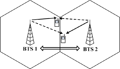
Figure 1: A scenario with two base transceiver stations and two mobiles.

We optimize the powers allocated across the data streams and associated beamformers with multiple transmit antennas with cooperative transmissions for both narrowband and wideband scenarios. For narrowband channels with a single transmit antenna the frontier of the achievable rate region is computed by solving a linear-fractional program. The weighted sum rate can be maximized by comparing at most six extremal rate pairs in the constraint set for transmit power. With multiple transmit antennas, the achievable rate region can be characterized by maximizing the weighted sum rate over the allocated power and the beamforming vector for each message, and the resulting optimization problem can be solved efficiently by numerical methods. This noncoherent cooperative scheme often achieves a significantly larger rate region and much higher sum rate than non-cooperative schemes.

With wideband (frequency-selective) channels, the power is allocated over multiple sub-carriers. Maximizing the sum rate is in general a non-convex problem. Under mild assumptions, however, the dual problem can be solved efficiently. Moreover, we propose a suboptimal power allocation scheme for the case of a single transmit antenna, which admits a simple analytical solution. This suboptimal scheme performs almost as well as the optimal power allocation when the direct- and cross-channel gains are of the same order.

The optimization problems presented can be easily extended to more than two BTSs and two mobiles. However, the structure of the solution becomes more complicated, necessitating general numerical (convex programming) techniques. Here we focus on the scenario with two mobiles in adjacent cells since in practice a particular mobile is likely to have only one relatively strong interferer, and coordinating among more than two mobiles across cells becomes quite complicated. (This complication can be compounded by the scheduler, which may reassign nearby mobiles different time-frequency resources over successive frames.) Finally, the two-mobile scenario provides significant insight into the potential gains of the cooperative scheme.

II Narrowband Cooperation Model

Consider downlink transmission in two adjacent cells each with the same set of narrowband channels. Within each cell, the signals from the BTS to its associated different mobiles occupy non-overlapping time-frequency resources; however, in each time-frequency slot, there can be inter-cell interference. Here we consider two mobiles in adjacent cells assigned the same narrowband channel. Assuming a narrowband system with block fading and single transmit antenna at each BTS and single receive antenna at each mobile, the baseband signal received by mobile $j\!=\!1,2$ during the $n$-th symbol interval is

$$y_{j}{(n)}=\sqrt{g_{j1}}e^{i\theta_{j1}(n)}x_{1}{(n)}+\sqrt{g_{j2}}e^{i\theta_{j2}(n)}x_{2}{(n)}+z_{j}{(n)},$$ (1)

where $i^{2}\!=\!-1$, $g_{jk}$ denotes the positive block fading gain from BTS $k$ to mobile $j$, $x_{k}{(n)}$, for $k\!=\!1,2$, denotes the transmitted signal from BTS $k$ at the $n$-th symbol interval, $\theta_{jk}(n)$ denotes the phase of the fading channel from BTS $k$ to mobile $j$, and $z_{j}{(n)}$ denotes the noise at mobile $j$, which is a sample from a sequence of independent, unit-variance circularly symmetric complex Gaussian (CSCG) random variables.

TABLE I: Knowledge of CSI at each terminal.

	$g_{11}$	$g_{21}$	$g_{12}$	$g_{22}$	$\theta_{11}(n)$	$\theta_{21}(n)$	$\theta_{12}(n)$	$\theta_{22}(n)$
BTS 1	Y	Y	Y	Y			N	N
BTS 2	Y	Y	Y	Y	N	N
mobile 1	Y		Y		Y		Y
mobile 2		Y		Y		Y		Y

It is important to specify what channel state information is known to which transmitters and/or receivers. The block fading gains $(g_{11},g_{21},g_{12},g_{22})$ are known to both BTSs. The gains $(g_{j1},g_{j2})$ are known to the corresponding receiver $j$. Usually, these gains are measured by the receiver and sent back to the transmitters through some feedback link. Whether $(g_{j1},g_{j2})$ are known to the other receiver is inconsequential in this study. The phases $\big{(}\theta_{j1}(n),\theta_{j2}(n)\big{)}$ are known or can be acquired by mobile $j$. Phases $\big{(}\theta_{11}(n),\theta_{21}(n)\big{)}$ from BTS 1 are unknown to BTS 2. Likewise, phases $\big{(}\theta_{12}(n),\theta_{22}(n)\big{)}$ are unknown to BTS 1. In fact, due to the frequency offset between the two oscillators at the two BTSs, the phase difference $\theta_{j1}(n)-\theta_{j2}(n)$ varies rapidly with $n$ at each mobile $j$. This prohibits one BTS to track the phases originating from the other BTS. Hence coherent combining at the receiver is not feasible. Since receiver $j$ can compensate for phase $\theta_{jj}(n)$, it can be assumed without loss of generality that $\theta_{11}(n)\!=\!\theta_{22}(n)\!=\!0$, where $\theta_{21}(n)$ and $\theta_{12}(n)$ denote the rapidly varying phase differences. The preceding assumptions are summarized in Table I, where an entry “Y” (respectively “N”) means the CSI in the corresponding column is known (respectively unknown) to the terminal in the corresponding row, and an empty entry means whether the corresponding CSI is known to the terminal is inconsequential.

It is assumed that a dedicated link between the two BTSs allows sharing of their messages, and allocation of powers across streams and code rates may be determined at a BTS or a separate radio control node. Each BTS is subject to its own power constraint.

The proposed cooperation consists of three techniques:

II-1 Message Sharing and Rate-Splitting

Each BTS has a message for its assigned mobile, and each BTS may split its message into two parts, where one part is to be transmitted by itself, and the other part is shared with and transmitted by the other BTS. This splits the data stream intended for each mobile. This implies partial message sharing across the two BTSs, which reduces the burden on the backhaul link relative to full message sharing.

II-2 Superposition Coding

Each BTS has its own message intended for its assigned mobile, and possibly also the shared message from the other BTS. The two messages are encoded separately. Let the message transmitted by BTS $k$ and intended for mobile $j$ be encoded as $\big{(}x_{jk}{(1)},\ldots,x_{jk}{(N)}\big{)}$ so that the superposition $x_{k}{(n)}\!=\!x_{1k}{(n)}\!+\!x_{2k}{(n)}$ is transmitted by BTS $k$. Then the received signal by mobile $j\!=\!1,2$ during the $n$-th symbol interval can be rewritten as

$$y_{j}{(n)}=\sqrt{g_{j1}}e^{i\theta_{j1}(n)}\big{[}x_{11}{(n)}+x_{21}{(n)}\big{]}+\sqrt{g_{j2}}e^{i\theta_{j2}(n)}\big{[}x_{12}{(n)}+x_{22}{(n)}\big{]}+z_{j}{(n)}$$ (2)

and the per-BTS power constraints can be stated as

$$\frac{1}{N}\sum_{n=1}^{N}\big{[}|x_{1k}(n)|^{2}+|x_{2k}(n)|^{2}\big{]}\leq P_{k},~{}k=1,2.$$ (3)

II-3 Interference Cancellation

Each mobile receives the desired signal, an interference signal, and noise. Both the desired and interference signals may come from two BTSs. Here we assume that each mobile treats the interference signal as noise and does not attempt to decode the messages intended for the other mobile, since one mobile may not be aware of the modulation and coding scheme of the signals intended for the other mobile.

Each mobile decodes its two messages, one from each BTS, possibly using successive decoding, i.e., it can first decode the message from one BTS and completely cancel the self-interference when decoding the message from the other BTS. With this scheme the two-transmitter two-receiver channel can be viewed as two mutually interfering multiaccess channels (MACs), where each MAC consists of one mobile receiver and both BTS transmitters.

Throughout this paper, we assume standard Gaussian codebooks (although those may not be optimal in this scenario), which do not require phase synchronization among the two cooperating transmitters.

III Narrowband Rate Region

III-A The Rate Region Frontier

Given the channel gains $\boldsymbol{g}\!=\!(g_{11},g_{21},g_{12},g_{22})$ and power constraints $\boldsymbol{P}\!=\!(P_{1},P_{2})$, the achievable rate region is defined as the convex hull of the following region

$$\mathcal{R}(\boldsymbol{g},\boldsymbol{P})\triangleq\bigg{\{} (R_{1},R_{2})\bigg{\arrowvert}\begin{matrix}R_{1}=\log\big{(}1+\frac{g_{11}P_{11}+g_{12}P_{12}}{1+g_{11}P_{21}+g_{12}P_{22}}\big{)}\\ R_{2}=\log\big{(}1+\frac{g_{21}P_{21}+g_{22}P_{22}}{1+g_{21}P_{11}+g_{22}P_{12}}\big{)}\end{matrix}$$ (4)

$$\text{for some}~{}P_{11},P_{12},P_{21},P_{22}\!\geq\!0~{}\text{satisfying}~{}P_{11}\!+\!P_{21}\!\leq\!P_{1}~{}\text{and}~{}P_{12}\!+\!P_{22}\!\leq\!P_{2}\bigg{\}},$$

where $P_{jk}$ is the power BTS $k$ allocates to mobile $j$. (It is not difficult to check that $\mathcal{R}(\boldsymbol{g},\boldsymbol{P})$ is indeed a region.) To find the frontier of $\mathcal{R}(\boldsymbol{g},\boldsymbol{P})$, we maximize the rate of user 2 for a given rate of user 1. By sweeping the rate of user 1 over all possible values, we obtain the trade-off between the two users’ rates (without time sharing), which is referred to as the rate region frontier. From the rate expression (4), the optimization problem is written as:

$$\underset{\{P_{jk}\}}{\operatorname{\text{maximize}}}~{}~{} R_{2}=\log\bigg{(}1+\frac{g_{21}P_{21}+g_{22}P_{22}}{1+g_{21}P_{11}+g_{22}P_{12}}\bigg{)}$$ (5a)

subject to $$\log\bigg{(}1+\frac{g_{11}P_{11}+g_{12}P_{12}}{1+g_{11}P_{21}+g_{12}P_{22}}\bigg{)}=R_{1}$$ (5b)

$$P_{1k}+P_{2k}\leq P_{k},~{}~{}~{}P_{jk}\geq 0,~{}j,k=1,2.$$ (5c)

Since $\log(\cdot)$ is an increasing function, the rate objective (5a) is equivalently the argument of the logarithm function. The constraint (5b) is linear in the variables. Hence this optimization problem is a linear-fractional program [25]. Specifically, letting $Z\!=\!1\!+\!g_{21}P_{11}\!+\!g_{22}P_{12}$ and

$$P_{jk}=\frac{\widetilde{P}_{jk}}{Z},~{}j,k=1,2,$$ (6)

Problem (5) can be rewritten as the following equivalent linear program:

$$\underset{\{\widetilde{P}_{jk}\},~{}Z}{\operatorname{\text{maximize}}}~{}~{} g_{21}\widetilde{P}_{21}+g_{22}\widetilde{P}_{22}$$ (7a)

subject to $$g_{11}\widetilde{P}_{11}+g_{12}\widetilde{P}_{12}-(2^{R_{1}}-1)(g_{11}\widetilde{P}_{21}+g_{12}\widetilde{P}_{22}+Z)=0$$ (7b)

$$\widetilde{P}_{1k}+\widetilde{P}_{2k}-P_{k}Z\leq 0,~{}k=1,2$$ (7c)

$$g_{21}\widetilde{P}_{11}+g_{22}\widetilde{P}_{12}+Z=1,~{}~{}~{}\widetilde{P}_{jk},Z\geq 0,~{}j,k=1,2.$$ (7d)

From [25, Ch. 4], it can be shown that the optimal $Z\!>\!0$. The optimal power $P_{jk}$ in Problem (5) is given by (6), where $\widetilde{P}_{jk}$ and $Z$ are obtained from the linear program in (7), which can be solved efficiently using standard techniques [25].

The rate region frontier can then be computed by solving a family of linear-fractional programs corresponding to sweeping over the valid range of $R_{1}$. It is easy to show that the valid range of $R_{j}$ is the interval $\big{[}0,\log(1\!+\!g_{j1}P_{1}\!+\!g_{j2}P_{2})\big{]}$.

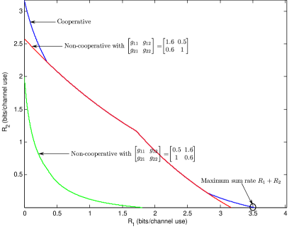
Figure 2: The rate region frontiers achieved by cooperative and non-cooperative schemes with $P_{1}\!=\!P_{2}\!=\!5$.

Fig. 2 illustrates the rate region frontiers achieved by the cooperative scheme described in Section II, and by joint power control (without data sharing) as proposed in [20]. Two examples are shown. In the first, the direct-channel gains are stronger than the cross-channel gains. The cooperative scheme achieves noticeable gains over the non-cooperative scheme only when $R_{1}$ or $R_{2}$ is near zero. In the second example, the direct- and cross-channel gains are swapped, so that the cross-channel gains are stronger. The rate region achieved without cooperation becomes much smaller, while the rate region achieved with cooperation remains the same. Hence the gain due to cooperation in this scenario is mainly due to BTS selection.

The following lemma characterizes the optimal power allocation for points on the rate region frontier. We first observe that at least one of the constraints in (5c) must be binding, because otherwise increasing all $\{P_{jk}\}$ proportionally increases both $R_{1}$ and $R_{2}$.

Lemma 1

Every $(R_{1},R_{2})$ on the rate region frontier is achieved by a power allocation that satisfies

$$\begin{cases}P_{1k}+P_{2k}=P_{k},~{}&\text{if}~{}(2^{R_{1}}\!-\!1)(2^{R_{2}}\!-\!1)\leq 1\\ P_{1k}P_{2k}=0,~{}&\text{if}~{}(2^{R_{1}}\!-\!1)(2^{R_{2}}\!-\!1)>1\end{cases}$$ (8)

for $k\!=\!1,2$.

The proof is given in the appendix. If $R_{1}$ or $R_{2}$ is small enough such that $(2^{R_{1}}\!-\!1)(2^{R_{2}}\!-\!1)\!\leq 1\!$, then both BTSs transmit with full power. There may be points on the rate region frontier that satisfy $(2^{R_{1}}\!-\!1)(2^{R_{2}}\!-\!1)\!>\!1$, which implies $R_{1}\!>\!0$ and $R_{2}\!>\!0$. Each BTS then either transmits only its own message or only the shared message from the other BTS. These observations provide an easy way to compute the maximum weighted sum rate, as shown in the next section.

III-B Weighted Sum Rate Maximization

Consider the problem of maximizing the weighted sum rate

$$R(\mu)\triangleq R_{1}+\mu R_{2},$$ (9)

where the user rates are given by (4) and $\mu\!\geq\!0$ is the relative priority assigned to the second mobile and allows for a tradeoff between the overall system throughput and user fairness. For given $\mu$, the maximum of $R(\mu)$ is always achieved by some rate pair on the rate region frontier. For every $\mu$, (9) describes a straight line in the $(R_{1},R_{2})$ plane, which is an outer bound on the rate region. The intersection of the regions below all such outer bounds is exactly the achievable rate region, which is the convex hull of the region under the rate region frontier. Any rate pair in this rate region can be achieved by time sharing two rate pairs on the rate region frontier found in Section III.A.

Proposition 1

The maximum of $R_{1}\!+\!R_{2}$ is achieved at one of the four corner points listed in Table II.

The four corner points of the power constraint set shown in Table II correspond to full cooperation, meaning that both BTSs cooperatively transmit with full power to one mobile or each BTS only transmits the shared message from the other BTS, and non-cooperation, meaning that each BTS transmits to its own mobile with full power and without rate-splitting.

TABLE II: Corner points and possible stationary points for weighted sum rate maximization.

		$P_{11}$	$P_{21}$	$P_{12}$	$P_{22}$
corner points	full cooperation	$P_{1}$	$0$	$P_{2}$	$0$
		$0$	$P_{1}$	$0$	$P_{2}$
		$0$	$P_{1}$	$P_{2}$	$0$
	non-cooperation	$P_{1}$	$0$	$0$	$P_{2}$
stationary points	$\mu>1$	$P_{11}^{*}$	$0$	$0$	$P_{2}$
		$0$	$P_{1}$	$P_{12}^{*}$	$0$
	$\mu<1$	$P_{1}$	$0$	$0$	$P_{22}^{*}$
		$0$	$P_{21}^{*}$	$P_{2}$	$0$

Proposition 2

If $\mu\!\neq\!1$, then the power allocation, which maximizes $R_{1}\!+\mu\!R_{2}$ satisfies $P_{1k}P_{2k}\!=\!0$ for $k\!=\!1,2$, and has the form shown in Table II where $P_{jk}^{*}\!<\!P_{k}$.

Proof:

The proofs of Propositions 1 and 2 consist of examining the stationary points associated with the two conditions in Lemma 1. (Note that there must exist a point on the rate frontier that achieves sum rate $R(\mu)$.) We first show that if $(2^{R_{1}}\!-\!1)(2^{R_{2}}\!-\!1)\leq 1$, then $R(\mu)$ achieves its maximum at one of the four corner points listed in Table II. From (4) and Lemma 1, we have

$$R(\mu)=\log\bigg{[}\frac{1+g_{11}P_{1}+g_{12}P_{2}}{1+g_{11}(P_{1}-P_{11})+g_{12}(P_{2}-P_{12})}\bigg{]}+\mu\log\bigg{[}\frac{1+g_{21}P_{1}+g_{22}P_{2}}{1+g_{21}P_{11}+g_{22}P_{12}}\bigg{]}.$$ (10)

It is easy to show that for any fixed $P_{12}$, $\frac{\partial R(\mu)}{\partial P_{11}}$ is increasing with $P_{11}$ so that $R(\mu)$ is maximized at an extreme value for $P_{11}$. More generally, it is straightforward to show that $\frac{\partial R(\mu)}{\partial P_{jk}}$ is increasing with $P_{jk}$ for all $j$ and $k$. Hence $R(\mu)$ is maximized at one of the extreme points of the power constraint set.

To find stationary points on the rate region frontier satisfying $(2^{R_{1}}\!-\!1)(2^{R_{2}}\!-\!1)\!>\!1$, Lemma 1 states that we can assume $P_{1k}P_{2k}\!=\!0$. In general, the rate region frontier may not contain points satisfying the condition $(2^{R_{1}}\!-\!1)(2^{R_{2}}\!-\!1)\!>\!1$. In that case, the power allocation schemes satisfying $P_{kk}P_{jk}\!=\!0$ must be suboptimal. However, without knowing the rate pairs on the frontier, we can assume this condition is satisfied and characterize the stationary points, which then serve as candidate points for achieving the maximum weighted sum rate. This gives two possible frontiers corresponding to the two types of power allocations in Table II. Namely, one candidate frontier is obtained by fixing $P_{22}\!=\!P_{2}$ (or $P_{11}\!=\!P_{1}$) and sweeping the value of $P_{11}$ (or $P_{22}$) across the interval $[0,P_{1}]$ (or $[0,P_{2}]$). The other candidate frontier is obtained by fixing $P_{21}\!=\!P_{1}$ (or $P_{12}\!=\!P_{2}$) and sweeping the value of $P_{12}$ (or $P_{21}$) over the interval $[0,P_{2}]$ (or $[0,P_{1}]$). The actual rate frontier is then the maximum of the two candidate frontiers.

For the first candidate frontier we have

$$R(\mu)=\log\bigg{(}1+\frac{g_{11}P_{11}}{1+g_{12}P_{2}}\bigg{)}+\mu\log\bigg{(}1+\frac{g_{22}P_{2}}{1+g_{21}P_{11}}\bigg{)}.$$ (11)

Examining $\frac{dR(\mu)}{dP_{11}}$, the maximizing value $P_{11}^{*}$ is the solution to the quadratic equation $a_{1}P_{11}^{2}\!+\!b_{1}P_{11}\!+\!c_{1}\!=\!0$, where $a_{1}\!=\!g_{11}g_{21}^{2}\!>\!0$, $b_{1}\!=\!2g_{11}g_{21}\!+\!(1-\mu)g_{11}g_{21}g_{22}P_{2}$, and $c_{1}\!=\!g_{11}(1\!+\!g_{22}P_{2})\!-\!\mu g_{21}g_{22}P_{2}(1\!+\!g_{12}P_{2})$. Since $a_{1}\!>\!0$, the smaller root is the solution. It is easy to check that if $\mu$, $g_{jk}$, and $P_{2}$ satisfy $b_{1}^{2}\!-\!4a_{1}c_{1}\!\geq\!0$ and $0\!<\!P_{11}^{*}\!<\!P_{1}$, then $P_{11}^{*}$ achieves the maximum $R(\mu)$. Similarly, we could fix $P_{11}\!=\!P_{1}$ and optimize over $P_{22}$. The resulting necessary conditions show that if $\mu\!>\!1$ (or $\mu\!<\!1$), then maximizing over $P_{11}$ (or $P_{22}$) gives a candidate stationary point, as stated in Proposition 2. A similar argument shows that if $\mu\!>\!1$ (or $\mu\!<\!1$), then maximizing over $P_{12}$ (or $P_{21}$) gives a second candidate stationary point on the frontier.

If $\mu\!=\!1$, then $b_{1}\!>\!0$, which implies that $P_{11}^{*}\!<\!0$ (if it is real). It can be similarly verified for the other cases that there are no valid stationary points in the interior of the power constraint set, which establishes Proposition 1. ∎

The preceding propositions state that the maximum weighted sum rate can be efficiently determined by searching over the small number of candidate power allocations shown in Table II. This will be used as the basis for optimizing wideband power allocations discussed in the next section.

IV Frequency-Selective Channels

IV-A Problem Formulation

We now consider a wideband system with frequency-selective channels. A wideband channel is modeled as a set of $L$ discrete (parallel) channels. Each sub-channel is modeled similarly as (1), with the same CSI known at the terminals. Instead of one power constraint for each sub-channel, the $L$ sub-channels are subject to a total power constraint at each BTS. The problem is to maximize the weighted sum across users of the rates summed across sub-channels:

$$\underset{\{P_{jk}(l),P_{k}(l)\}}{\operatorname{\text{maximize}}} ~{}~{}\sum_{l=1}^{L}\big{[}R_{1}(l)+\mu R_{2}(l)\big{]}$$ (12a)

subject to $$~{}~{}P_{1k}(l)+P_{2k}(l)\leq P_{k}(l),~{}\forall k,l$$ (12b)

$$~{}~{}\sum_{l=1}^{L}P_{k}(l)\leq P_{\text{tot},k},~{}~{}~{}P_{jk}(l)\geq 0,~{}~{}~{}P_{k}(l)\geq 0,~{}~{}~{}\forall j,k,l,$$ (12c)

where $l$ denotes the sub-channel index, $P_{k}(l)$ denotes the power allocated to sub-channel $l$, and $P_{\text{tot},k}$ denotes the total power constraint at BTS $k$. Rates $R_{1}(l)$ and $R_{2}(l)$ are given by (4), where the channel gains $g_{jk}$ and powers depend on $l$.

This can be viewed as a two-level optimization problem. At the lower level the weighted sum rate is maximized for each sub-channel given its allocated power. The upper level then optimizes the power allocation across sub-channels subject to the total power constraints. Based on the discussion in the last section, the maximum rate for each sub-channel is achieved by one of the cases in Table II. In general, solving the two-level problem requires iterating between the lower- and upper-levels.

The three cooperative power assignments in Table II give the following weighted sum rates for sub-channel $l$:

$$R_{1}^{(\text{c})}(l)\triangleq \log\big{[}1+g_{11}(l)P_{1}(l)+g_{12}(l)P_{2}(l)\big{]}$$ (13)

$$R_{2}^{(\text{c})}(l)\triangleq \mu\log\big{[}1+g_{21}(l)P_{1}(l)+g_{22}(l)P_{2}(l)\big{]}$$ (14)

$$R_{3}^{(\text{c})}(l)\triangleq \log\bigg{[}1+\frac{g_{12}(l)P_{2}(l)}{1+g_{11}(l)P_{1}(l)}\bigg{]}+\mu\log\bigg{[}1+\frac{g_{21}(l)P_{1}(l)}{1+g_{22}(l)P_{2}(l)}\bigg{]},$$ (15)

whereas the non-cooperative assignment gives

$$R^{\text{(nc)}}(l)\triangleq\log\bigg{[}1+\frac{g_{11}(l)P_{1}(l)}{1+g_{12}(l)P_{2}(l)}\bigg{]}+\mu\log\bigg{[}1+\frac{g_{22}(l)P_{2}(l)}{1+g_{11}(l)P_{1}(l)}\bigg{]}.$$ (16)

The power control problem is then

$$\underset{\{P_{k}(l)\}}{\operatorname{\text{maximize}}}~{}~{}\sum_{l=1}^{L}\max\bigg{\{}R_{1}^{(\text{c})}(l),R_{2}^{(\text{c})}(l),R_{3}^{(\text{c})}(l),R^{(\text{nc})}(l)\bigg{\}}$$ (17)

subject to (12c).

Note that the rate objective includes only the corner points and does not explicitly include the interior points (stationary points). However, the interior points are implicitly included in the rate objective due to the power optimization at the upper level. Namely, if the weighted sum rate for sub-channel $l$ is maximized at an interior point, e.g., corresponding to $P_{11}^{*}(l)\!<\!\overline{P}_{1}(l)$, $P_{22}(l)\!=\!\overline{P}_{2}(l)$, $P_{12}(l)\!=\!P_{21}(l)\!=\!0$, where $\overline{P}_{k}(l)$ is the $l$-th sub-channel power constraint at BTS $k$, then the rate can be increased by decreasing $\overline{P}_{1}(l)$ via the upper-level optimization.

IV-B Continuous Power Allocation

Problem (17) is non-convex in general because of the non-convexity of the objective function. However, letting the number of sub-carriers within a given band $F$ go to infinity, we can assume that $g_{jk}(l)$ converges to a continuous function of frequency $f\!\in\!F$, and the corresponding continuous optimization problem can be efficiently solved numerically. The continuous optimization problem can be formulated as

$$\underset{\{P_{k}(f)\}}{\operatorname{\text{maximize}}} ~{}~{}\int_{F}\max\bigg{\{}R_{1}^{(\text{c})}(f),R_{2}^{(\text{c})}(f),R_{3}^{(\text{c})}(f),R^{(\text{nc})}(f)\bigg{\}}df$$ (18a)

subject to $$~{}~{}\int_{F}P_{k}(f)df\leq P_{\text{tot},k},~{}~{}~{}P_{k}(f)\geq 0,~{}\forall k,f,$$ (18b)

where the index $l$ is replaced by the continuous variable $f$.

Definition [26]: Consider the general optimization problem:

maximize $$~{}~{}\sum_{n=1}^{N}f_{n}(\boldsymbol{x}_{n})$$ (19a)

subject to $$~{}~{}\sum_{n=1}^{N}\boldsymbol{h}_{n}(\boldsymbol{x}_{n})\leq\boldsymbol{P},$$ (19b)

where $\boldsymbol{x}_{n}\in\mathbb{R}^{K}$ are the optimization variables, each function $f_{n}(\cdot)\!:~{}\mathbb{R}^{K}\!\rightarrow\!\mathbb{R}$ is not necessarily concave, and each function $\boldsymbol{h}_{n}(\cdot)\!\!:\mathbb{R}^{K}\!\rightarrow\!\mathbb{R}^{L}$ is not necessarily convex. Power constraints are denoted by an $L$-vector $\boldsymbol{P}$. Here, “$\leq$” is used to denote a component-wise inequality. An optimization problem of the form (19) is said to satisfy the time-sharing condition if for any $\boldsymbol{P}_{\boldsymbol{x}}$, $\boldsymbol{P}_{\boldsymbol{y}}$ with corresponding optimal solutions $\boldsymbol{x}_{n}^{*}$ and $\boldsymbol{y}_{n}^{*}$, respectively, and for any $0\leq v\leq 1$, there exists a feasible solution $\boldsymbol{z}_{n}$, such that $\sum_{n=1}^{N}\boldsymbol{h}_{n}(\boldsymbol{z}_{n})\leq\nu\boldsymbol{P}_{\boldsymbol{x}}+(1-\nu)\boldsymbol{P}_{\boldsymbol{y}}$, and $\sum_{n=1}^{N}f_{n}(\boldsymbol{z}_{n})\geq\nu\sum_{n=1}^{N}f_{n}(\boldsymbol{x}_{n}^{*})+(1-\nu)\sum_{n=1}^{N}f_{n}(\boldsymbol{y}_{n}^{*})$.

The time-sharing condition essentially states that the optimal value of the objective in (19) is concave in $\boldsymbol{P}$. It is shown in [26] that if the time-sharing condition is satisfied, then the optimization problem has zero duality gap, i.e., solving the dual problem gives the same optimal value as solving the primal problem even if it is not convex.

Since $g_{jk}(f)$ is continuous in $f$, $R_{i}^{(\text{c})}(f),~{}i\!=\!1,2,3$ and $R^{(\text{nc})}(f)$ are continuous in $f$, and the integrand of the objective function is continuous in $f$. Therefore, we can apply the techniques used in the proof of Theorem 2 in [26] to show that this optimization problem satisfies the time-sharing condition. Then the optimization problem (18) has zero duality gap and for this problem solving its dual is more efficient.

The solution to Problem (18) approximates the solution to (17) and it becomes more accurate as $L\!\rightarrow\!\infty$. In practical systems with a large number of sub-carriers, the channel gains between consecutive sub-carriers are typically highly correlated. Hence we expect that the time-sharing condition is approximately satisfied for (17), so that the solution to the dual problem will be nearly-optimal.

The Lagrangian function associated with Problem (17) is

$$L(\boldsymbol{P}_{1}, \boldsymbol{P}_{2},\boldsymbol{\lambda})=\sum_{l=1}^{L}\max\bigg{\{}R_{1}^{(\text{c})}(l),R_{2}^{(\text{c})}(l),R_{3}^{(\text{c})}(l),R^{(\text{nc})}(l)\bigg{\}}$$

$$-\lambda_{1}\bigg{(}\sum_{l=1}^{L}P_{1}(l)-P_{\text{tot},1}\bigg{)}-\lambda_{2}\bigg{(}\sum_{l=1}^{L}P_{2}(l)-P_{\text{tot},2}\bigg{)},$$ (20)

where $\lambda_{k}\!\geq\!0$ is the Lagrange multiplier associated with the power constraint for BTS $k$ and the bold-font denotes the vector version of the corresponding variables. The dual optimization problem associated with Problem (17) is

$$\underset{\lambda_{1},\lambda_{2}}{\operatorname{\text{minimize}}}~{}~{}g(\boldsymbol{\lambda})~{}~{}\text{subject to}~{}\lambda_{1}\geq 0,~{}\lambda_{2}\geq 0,$$

where

$$g(\boldsymbol{\lambda})=\displaystyle{\max_{\boldsymbol{P}_{1},\boldsymbol{P}_{2}}}L(\boldsymbol{P}_{1},\boldsymbol{P}_{2},\boldsymbol{\lambda})$$ (21)

is the dual objective function.

Compared with numerically solving the primal problem (17) directly, two properties of the dual problem lead to a reduction in computational complexity. One is that for any fixed $\boldsymbol{\lambda}$, the solution to (21) can be computed per-sub-carrier since (21) can be decomposed into $L$ parallel unconstrained optimization problems. Note that for each sub-carrier an exhaustive search for the optimal $P_{k}(l)$ must be carried out. The other property is the dual problem is convex in the variables $\boldsymbol{\lambda}$, which guarantees the convergence of numerical methods. In the numerical results that follow we solve the dual optimization problem efficiently via a nested bisection search over $\lambda_{1}$ and $\lambda_{2}$ [26, 27]. (An outer loop updates $\lambda_{1}$ and an inner loop updates $\lambda_{2}$.) If the required accuracy of each $\lambda$ is given by $\epsilon_{\lambda}$, then the overall computational complexity of the bisection search is $\mathcal{O}(L\log(1/\epsilon_{\lambda})^{2})$, which is linear in $L$ [27].

IV-C High-SNR Approximation with $\mu\!=\!1$

At high signal-to-noise ratios (SNRs), we have $R_{i}^{(\text{c})}\!>\!R^{(\text{nc})}$ and $R_{i}^{(\text{c})}\!>\!R_{3}^{(\text{c})}$ for $i\!=\!1,2$, since $R^{(\text{nc})}$ and $R_{3}^{(\text{c})}$ are interference-limited. Hence we can simplify Problem (18) by maximizing over only $R_{i}^{(\text{c})}$, $i\!=\!1,2$, in the integrand of the rate objective. The corresponding suboptimal power allocation problem can be written as

$$\underset{\{P_{k}(f)\}}{\operatorname{\text{maximize}}}~{}~{}\int_{F}\max\bigg{\{}R_{1}^{(\text{c})}(f),R_{2}^{(\text{c})}(f)\bigg{\}}df$$ (22)

subject to (18b). This is still a two-level optimization problem. The lower level selects the better MAC channel from the two options for each sub-carrier, and the upper level distributes the power to each sub-carrier subject to the total power constraint.

Although $R_{1}^{(\text{c})}(f)$ and $R_{2}^{(\text{c})}(f)$ are concave functions of $P_{1}(f)$ and $P_{2}(f)$, $\max\big{\{}R_{1}^{(\text{c})}(f),R_{2}^{(\text{c})}(f)\big{\}}$ is in general not concave in $P_{1}(f)$ and $P_{2}(f)$. Problem (22) can be efficiently solved as described in the last subsection (via its dual problem); however, it turns out that under some mild conditions it can be transformed into a convex program so that standard efficient numerical techniques can also be applied.

Specifically, we solve this problem by finding a convex function that upper bounds $\max\big{\{}R_{1}^{(\text{c})}(f),$
$R_{2}^{(\text{c})}(f)\big{\}}$, and optimizing this upper bound over the power allocations. It can be shown that substituting the optimized power allocation for the upper bound into the original objective in (22) gives the same value as the optimized upper bound.

Letting

$$R_{\text{ub}}(f)\triangleq\log\big{[}1+\max\{g_{11}(f),g_{21}(f)\}P_{1}(f)+\max\{g_{12}(f),g_{22}(f)\}P_{2}(f)\big{]},$$ (23)

we observe that $R_{\text{ub}}(f)$ serves as a pointwise upper bound for any full-cooperation scheme, i.e.,

$$\max\bigg{\{}R_{1}^{(\text{c})}(f),R_{2}^{(\text{c})}(f)\bigg{\}}\leq R_{\text{ub}}(f),~{}\forall f.$$ (24)

We now consider the optimization problem

$$\underset{\{P_{k}(f)\}}{\operatorname{\text{maximize}}}~{}~{}\int_{F}R_{\text{ub}}(f)df$$ (25)

subject to (18b). Since $R_{\text{ub}}(f)$ is concave with respect to $P_{1}(f)$ and $P_{2}(f)$, Problem (25) is a convex optimization problem. Therefore the necessary Karush-Kuhn-Tucker (KKT) conditions for optimality are also sufficient. Letting $y_{k}(f)\!=\!1/\max\{g_{1k}(f),g_{2k}(f)\}$, the KKT conditions for the optimal power allocation, $P_{1}^{*}(f)$ and $P_{2}^{*}(f)$, can be stated as

$$\text{a}.~{} \text{If}~{}\lambda_{1}y_{1}(f)<\lambda_{2}y_{2}(f),~{}\text{then}$$

$$P_{1}^{*}(f)=\bigg{(}\frac{1}{\lambda_{1}}-y_{1}(f)\bigg{)}^{+},~{}P_{2}^{*}(f)=0$$

$$\text{b}.~{} \text{If}~{}\lambda_{1}y_{1}(f)>\lambda_{2}y_{2}(f),~{}\text{then}$$

$$P_{1}^{*}(f)=0,~{}P_{2}^{*}(f)=\bigg{(}\frac{1}{\lambda_{2}}-y_{2}(f)\bigg{)}^{+}$$

$$\text{c}.~{} \text{If}~{}\lambda_{1}y_{1}(f)=\lambda_{2}y_{2}(f),~{}\text{then}$$

$$P_{1}^{*}(f)+\frac{y_{1}(f)}{y_{2}(f)}P_{2}^{*}(f)=\bigg{(}\frac{1}{\lambda_{1}}-y_{1}(f)\bigg{)}^{+},~{}P_{1}^{*}(f),P_{2}^{*}(f)\geq 0,$$

where $(x)^{+}\!\triangleq\!\max\{x,0\}$, $\lambda_{1}$ and $\lambda_{2}$ are non-negative and can be determined by substituting the optimal power allocation into the power constraints.

For a given set of channel fading gains $\boldsymbol{g}_{f}$, the optimal power allocation is not unique only for the preceding Case c. Assuming the joint distribution of the channel gains is continuous (e.g., Rayleigh fading), this happens with probability zero. Therefore with probability one the optimal power allocation is unique and is determined by the first two conditions. The optimal power control scheme implies that only one BTS is assigned to transmit at any given $f$, i.e., the BTS with relatively stronger direct- or cross-channel gains. The two-level water-filling structure of the power allocation indicates that orthogonal transmission is optimal and the gain of the cooperative scheme as considered here in the wideband channel comes from cell selection for each sub-channel, since for each sub-channel at most one link among the four direct- and cross-links between BTSs and mobiles is activated.

It is straightforward to show that substituting the optimized $P_{1}^{*}(f)$ and $P_{2}^{*}(f)$ in the objective in (22) gives the same result as substituting those functions into the corresponding upper bound $R_{\text{ub}}(f)$. This is because the solution states that only one BTS transmits at any given $f$. Since $P_{1}^{*}(f)$ and $P_{2}^{*}(f)$ maximize the upper bound, they must also maximize the original objective.

We observe that $\big{[}P_{1}^{*}(f),P_{2}^{*}(f)\big{]}$ is a KKT point for Problem (22). This is because when substituting $\big{[}P_{1}^{*}(f),P_{2}^{*}(f)\big{]}$ into the four rates listed in (13)–(16), the maximum value among the four rates is equal to the maximum value of the two cooperative rates in (13) and (14). Since $\big{[}P_{1}^{*}(f),P_{2}^{*}(f)\big{]}$ is a KKT point for Problem (22), it must also be a KKT point for Problem (18). This implies that $\big{[}P_{1}^{*}(f),P_{2}^{*}(f)\big{]}$ is a locally optimal power allocation scheme for (18) although it may not be globally optimal.

We emphasize that the equivalence between Problems (22) and (25) relies on the continuity of the integrand in the objective function. With a finite number of sub-carriers, the solutions to the two problems may not be the same. For example, with only one sub-carrier, by inspection the optimized objective in (25) is $\log\big{(}1\!+\!\max\{g_{11},g_{21}\}P_{\text{tot},1}\!+\!\max\{g_{12},g_{22}\}P_{\text{tot},2}\big{)}$, which cannot be achieved by (22) in general.

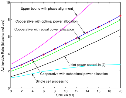
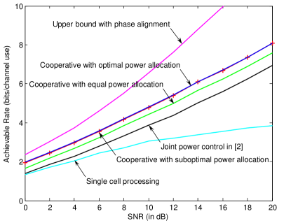
Figure 3: The achievable sum rate with: (a) equal direct- and cross-channel gains, i.e., $\mathbb{E}[g_{jk}]\!=\!1,~{}\forall j,k$; (b) direct-channels are 3 dB stronger than cross-channels, i.e., $\mathbb{E}[g_{jj}]\!=\!1,~{}j=1,2$ and $\mathbb{E}[g_{jk}]\!=\!0.5,~{}j,k\!=\!1,2,~{}j\neq k$.

In Fig. 3 we compare the maximum sum rates of the cooperative and non-cooperative schemes with wideband channels and $\mu\!=\!1$. For this example there are $L\!=\!128$ sub-carriers. The channels on each sub-carrier across the four direct- and cross-links undergo independent Rayleigh fading, and for each link the channels across sub-carriers are assumed to have correlation coefficients of $0.95$. The figure compares achievable rates for the following scenarios: 1) optimized power assignments across sub-carriers and both BTSs according to (18); 2) optimized power assignments across sub-carriers and both BTSs according to (22); 3) cooperation between BTSs with equal power assignments across sub-carriers; 4) both BTSs carry out joint power control but do not assist each other with data transmissions [2]. The achievable downlink sum rate of perfect BTS cooperation with phase alignment is included for comparison. Fig. 3 shows results with equal-variance direct- and cross-channel gains, which corresponds to the scenario where the two mobiles are both located close to the cell boundary, and Fig. 3 shows results for the case where the cross-channel gains are 3 dB weaker than the direct-channel gains.

The results in Fig. 3 show that the cooperative scheme considered offers approximately 5 dB gain relative to non-cooperative joint power control scheme in [2]. Also, cooperation with wideband power allocation offers about one dB gain with respect to equal power allocation and there is negligible difference between the suboptimal and optimal wideband power allocations.

The cooperative scheme considered can only provide diversity gain, and therefore achieves only one degree of freedom (asymptotic slope of rate curves in Fig. 3). In contrast, if the BTSs can cooperate with phase alignment, then two degrees of freedom can be achieved as illustrated in the figure. The performance improvement due to cooperation diminishes if the average cross-channel gains become weaker than the direct gains, as illustrated in Fig. 3.

V Multiple Transmit Antennas

We now consider the case where each BTS has $N_{t}\!\geq\!2$ transmit antennas and each mobile has a single receive antenna. Assuming a narrowband system with block fading, the baseband signal received by mobile $j\!=\!1,2$ during the $n$-th symbol interval is

$$y_{j}{(n)}=\big{(}\boldsymbol{h}_{j1}e^{i\theta_{j1}(n)}\big{)}^{\dagger}\boldsymbol{x}_{1}{(n)}+\big{(}\boldsymbol{h}_{j2}e^{i\theta_{j2}(n)}\big{)}^{\dagger}\boldsymbol{x}_{2}{(n)}+z_{j}{(n)},$$ (26)

where $\boldsymbol{x}_{k}{(n)}$, for $k\!=\!1,2$, denotes the transmit signal vector of dimension $N_{t}\!\times\!1$ from BTS $k$, $\boldsymbol{h}_{jk}$ denotes the complex channel vector consisting of the fading coefficients from the transmit antennas at BTS $k$ to the receive antenna at mobile $j$, and $\theta_{jk}(n)$ denotes the corresponding rapidly changing phase caused by the drifting frequency offset of the local oscillator. The same drift is experienced by all antennas. Similarly, it is assumed that the complex vectors $(\boldsymbol{h}_{j1},\boldsymbol{h}_{j2})$ are known to both BTSs and mobile $j$ and remain constant within one coding block, while the phases $\big{(}\theta_{j1}(n),\theta_{j2}(n)\big{)}$ are known to mobile $j$ and unknown to the other BTS. Without loss of generality, we can assume $\theta_{11}(n)\!=\!\theta_{22}(n)\!=\!0$ for all $n$.

V-A Cooperative Beamforming

In analogy with the single transmit antenna case, in the cooperative scheme each BTS splits its message into two parts, where one part is transmitted by itself and the other part is shared with and transmitted by the other BTS. Each BTS transmits a superposition of two codewords intended for the two mobiles and each codeword consists of scalar coding followed by beamforming, which can be written as

$$\boldsymbol{x}_{k}(n)=\boldsymbol{v}_{1k}x_{1k}{(n)}+\boldsymbol{v}_{2k}x_{2k}{(n)},~{}k=1,2,$$ (27)

where $\boldsymbol{v}_{jk}$ is a $N_{t}\!\times\!1$ vector with $\|\boldsymbol{v}_{jk}\|\!=\!1$, and denotes the normalized beamforming vector for the scalar symbol $x_{jk}$. The per-BTS power constraints are again given by (3). Each mobile decodes its two messages successively, treating signals for the other mobile as background noise. This scheme achieves the rate pair $(R_{1}^{(\text{bf})},R_{2}^{(\text{bf})})$ where

$$R_{k}^{(\text{bf})}=\log\bigg{(}1+\frac{|\boldsymbol{h}_{k1}^{\dagger}\boldsymbol{v}_{k1}|^{2}P_{k1}+|\boldsymbol{h}_{k2}^{\dagger}\boldsymbol{v}_{k2}|^{2}P_{k2}}{1+|\boldsymbol{h}_{k1}^{\dagger}\boldsymbol{v}_{j1}|^{2}P_{j1}+|\boldsymbol{h}_{k2}^{\dagger}\boldsymbol{v}_{j2}|^{2}P_{j2}}\bigg{)},~{}j\neq k.$$ (28)

Define $\bar{\boldsymbol{h}}_{jk}\!\triangleq\!\frac{\boldsymbol{h}_{jk}}{\|\boldsymbol{h}_{jk}\|}$ and $g_{jk}\!\triangleq\!\|\boldsymbol{h}_{jk}\|^{2}$. The optimal beamforming vector $\boldsymbol{v}_{jk}$ must lie in the space spanned by $\bar{\boldsymbol{h}}_{1k}$ and $\bar{\boldsymbol{h}}_{2k}$ [21], because any power spent on the null space of $\bar{\boldsymbol{h}}_{1k}$ and $\bar{\boldsymbol{h}}_{2k}$ will not be received by any mobile, and it does not have any impact on the signal-to-interference-plus-noise ratio (SINR) at each mobile. Fig. 4 illustrates the beamforming vector $\boldsymbol{v}_{11}$ geometrically in the plane spanned by $\bar{\boldsymbol{h}}_{11}$ and $\bar{\boldsymbol{h}}_{21}$, where $\alpha_{1}\!\triangleq\!\cos^{-1}\!\big{|}\bar{\boldsymbol{h}}_{11}^{\dagger}\bar{\boldsymbol{h}}_{21}\big{|}$ denotes the angle between $\bar{\boldsymbol{h}}_{11}$ and $\bar{\boldsymbol{h}}_{21}$, and $\beta_{11}$ denotes the angle between $\boldsymbol{v}_{11}$ and $\bar{\boldsymbol{h}}_{21}$. Then $\boldsymbol{v}_{11}$ can be parameterized as

$$\boldsymbol{v}_{11}=\frac{\cos{\beta_{11}}}{\cos{\alpha_{1}}}\boldsymbol{\Pi}_{\bar{\boldsymbol{h}}_{21}}\bar{\boldsymbol{h}}_{11}+\frac{\sin{\beta_{11}}}{\sin{\alpha_{1}}}\boldsymbol{\Pi}^{\bot}_{\bar{\boldsymbol{h}}_{21}}\bar{\boldsymbol{h}}_{11},$$ (29)

where $\boldsymbol{\Pi}_{\bar{\boldsymbol{h}}_{21}}\!\triangleq\!\bar{\boldsymbol{h}}_{21}\bar{\boldsymbol{h}}_{21}^{\dagger}$ and $\boldsymbol{\Pi}^{\bot}_{\bar{\boldsymbol{h}}_{21}}\!\triangleq\!\boldsymbol{I}\!-\!\boldsymbol{\Pi}_{\bar{\boldsymbol{h}}_{21}}$ denote the projection and orthogonal projection onto the column space of $\bar{\boldsymbol{h}}_{21}$, respectively, and the terms $\cos{\alpha_{1}}$ and $\sin{\alpha_{1}}$ in the corresponding denominators are used to normalize the two orthogonal vectors $\boldsymbol{\Pi}_{\bar{\boldsymbol{h}}_{21}}\bar{\boldsymbol{h}}_{11}$ and $\boldsymbol{\Pi}^{\bot}_{\bar{\boldsymbol{h}}_{21}}\bar{\boldsymbol{h}}_{11}$.

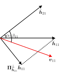
Figure 4: Illustration of the beamforming vector $\boldsymbol{v}_{11}$.

From (29), we can write $|\boldsymbol{h}_{11}^{\dagger}\boldsymbol{v}_{11}|^{2}\!=\!g_{11}\!\cos^{2}(\beta_{11}\!\!-\!\!\alpha_{1})$ and $|\boldsymbol{h}_{21}^{\dagger}\boldsymbol{v}_{11}|^{2}\!=\!g_{21}\!\cos^{2}\!\beta_{11}$. Similarly, the other three beamforming vectors can be parameterized by introducing $\alpha_{2}\!\triangleq\!\cos^{-1}\!\big{|}\bar{\boldsymbol{h}}_{12}^{\dagger}\bar{\boldsymbol{h}}_{22}\big{|}$ and $\beta_{jk}\in[0,\frac{\pi}{2}]$, $j,k=1,2$. The achievable rate pair $(R_{1}^{(\text{bf})},R_{2}^{(\text{bf})})$ can then be re-stated as

$$R_{k}^{(\text{bf})}\!=\!\log\bigg{[}1\!+\!\frac{g_{k1}\!\cos^{2}(\beta_{k1}\!\!-\!\!\alpha_{1})P_{k1}\!+\!g_{k2}\!\cos^{2}(\beta_{k2}\!\!-\!\!\alpha_{2})P_{k2}}{1\!+\!g_{k1}\!\cos^{2}\!\beta_{j1}P_{j1}\!+\!g_{k2}\!\cos^{2}\!\beta_{j2}P_{j2}}\bigg{]},~{}j\neq k.\\$$ (30)

Optimizing the beamforming vectors $\{\boldsymbol{v}_{jk}\}$ is now equivalent to optimizing the corresponding angles $\{\beta_{jk}\},~{}j,k\!=\!1,2$. If $\beta_{jk}\!=\!\alpha_{k}$ then BTS $k$ transmits to mobile $j$ with a maximum-ratio beamformer and if $\beta_{jk}\!=\!\frac{\pi}{2}$ then BTS $k$ transmits to mobile $j$ with a zero-forcing beamformer. In general, the optimal beamforming vectors must strike a balance between these two extremes. At high SNRs the solution should be close to zero-forcing, and at low SNRs the solution should be close to maximum-ratio combining. Note that with $N_{t}\!\geq 2\!$ antennas, the interference term in the denominator of (30) can be nulled out by choosing $\beta_{jk}\!=\!\frac{\pi}{2},~{}j,k\!=\!1,2$, therefore two degrees of freedom can be achieved.

V-B The Achievable Rate Region

The achievable rate region can be obtained by maximizing the weighted sum rate $R^{(\text{bf})}(\mu)\triangleq R_{1}^{(\text{bf})}+\mu R_{2}^{(\text{bf})},~{}\mu\geq 0$ over the beamforming vectors and the power allocated to each message for each $\mu$ and then sweeping $\mu$. To achieve a rate pair on the boundary of the rate region, the beams and powers must be jointly optimized. The following proposition states that both BTSs should always transmit with full power.

Proposition 3

For every rate pair $(R_{1}^{(\text{bf})},R_{2}^{(\text{bf})})$ on the boundary of the rate region, the corresponding power allocation satisfies $P_{1k}\!+\!P_{2k}\!=\!P_{k},~{}\forall k$.

Proof:

This follows from the observation that each beam contains a component, which is orthogonal to the cross-channel. Hence increasing power along that component increases the desired power without increasing interference. Specifically, let $\{\beta_{jk},P_{jk}\},j,k\!\!=\!\!1,2$ be the optimal parameters for a rate pair on the boundary of the rate region. From (30), the useful signal power from BTS $k$ to mobile $k$ is $g_{kk}\!\cos^{2}(\beta_{kk}\!\!-\!\!\alpha_{k})P_{kk}$ and the corresponding interference power is $g_{jk}\!\cos^{2}\!\beta_{kk}P_{kk}$, $j\!\neq\!k$. If $\beta_{kk}\!=\!\frac{\pi}{2}$, then increasing $P_{kk}$ will increase $R_{k}^{(\text{bf})}$ without changing $R_{j}^{(\text{bf})}$. If $\beta_{kk}\!\neq\!\frac{\pi}{2}$, then with fixed interference, i.e., $g_{jk}\!\cos^{2}\!\beta_{kk}P_{kk}\!=\!I$, the desired signal power can be expressed as $\frac{g_{kk}\!\cos^{2}(\beta_{kk}\!-\!\alpha_{k})I}{g_{jk}\!\cos^{2}\!\beta_{kk}}$, which is an increasing function of $\beta_{kk}$, implying that $P_{kk}$ should be maximized. Therefore the power constraint at BTS $k$ must be binding. ∎

Maximizing $R^{(\text{bf})}(\mu)$ is a non-convex problem; however, since there are only six variables to optimize it can be solved by exhaustive search optimally or by an iterative approach, in which the power allocation is optimized with fixed angles, the angles are optimized with fixed power allocation, and these two procedures are iterated until $R^{(\text{bf})}(\mu)$ converges. Note that convergence is guaranteed since $R^{(\text{bf})}(\mu)$ monotonically increases in each step, and is bounded due to the power limitations. The iterative approach can reduce the search complexity; however, optimality cannot be guaranteed although in our simulations global optimality was always observed.

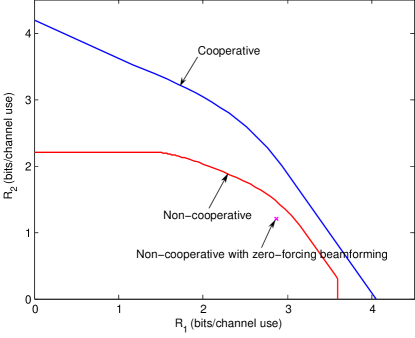
Figure 5: The rate region frontiers achieved by cooperative and non-cooperative schemes with $P_{1}\!=\!P_{2}\!=\!3$, $N_{t}\!=\!2$, and randomly generated channels.

Fig. 5 compares the rate region frontiers achieved by the cooperative scheme with the non-cooperative scheme presented in [21], in which the BTSs carry out joint beamforming and power control but do not share messages. Also shown is the rate pair achieved with zero-forcing transmission at each BTS without cooperation, i.e., BTS $k$ transmits to its own associated mobile $k$ with the orthogonal projection $\boldsymbol{I}\!-\!\boldsymbol{\Pi}_{\bar{\boldsymbol{h}}_{jk}},~{}j\!\neq\!k$. The figure shows that for this example BTS cooperation gives substantial gains in $R_{2}$ when $R_{1}$ is small.

V-C Frequency-Selective Channels

In a wideband system with frequency-selective channels that are modeled as a set of $L$ discrete channels, the cooperative beamforming and power control problem is given by

$$\underset{\{P_{jk}(l),\beta_{jk}(l)\}}{\operatorname{\text{maximize}}} ~{}~{}\sum_{l=1}^{L}\big{[}R_{1}^{(\text{bf})}(l)+\mu R_{2}^{(\text{bf})}(l)\big{]}$$ (31a)

subject to $$~{}~{}\sum_{l=1}^{L}\big{[}P_{1k}(l)+P_{2k}(l)\big{]}=P_{\text{tot},k},~{}~{}~{}P_{jk}(l)\geq 0,~{}\forall j,k,l,$$ (31b)

where $R_{k}^{(\text{bf})}(l)$ is given by (30), the channel gains $\{g_{jk}\}$, angles $\{\beta_{jk},\alpha_{k}\}$, and the powers depend on $l$, and the power constraints in (31b) are satisfied with equality due to Proposition 3.

As for a single antenna, this is again a two-level optimization problem. The lower level optimizes the beamforming vectors to maximize the weighted sum rate for each sub-channel given the power allocated to each message. The upper level then optimizes the power allocation across sub-channels for each message subject to the total power constraints.

Similar to the previous case with a single transmit antenna, the dual problem associated with Problem (31) can be formulated where the Lagrangian also depends on the angels $\{\boldsymbol{\beta}_{jk}\}$. (We omit the details due to space limitations.) As before, letting the number of sub-channels within a given band tend to infinity, we can assume that $g_{jk}(l)$ and $\alpha_{k}(l)$ converge to continuous functions of frequency $f$. The corresponding optimization problem over $\{P_{jk}(f)\}$ and $\{\beta_{jk}(f)\}$ has zero-duality gap and can be efficiently solved numerically. The numerical results in Fig. 6 were generated by solving the discrete version in (31) using a nested bisection search for $\boldsymbol{\lambda}$, where the maximization of the Lagrangian function in the inner loop is performed over the angles $\{\beta_{jk}(l)\},j,k=1,2$.

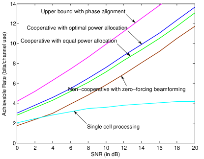
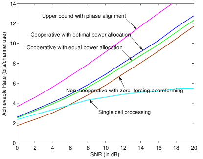
Figure 6: The achievable sum rate with $N_{t}\!=\!2$ and (a) equal direct- and cross-channel gains, i.e., $\mathbb{E}[g_{jk}]\!=\!1,~{}\forall j,k$; (b) direct-channels are 3 dB stronger than cross-channels, i.e., $\mathbb{E}[g_{jj}]\!=\!1,~{}j\!=\!1,2$ and $\mathbb{E}[g_{jk}]\!=\!0.5,~{}j,k\!=\!1,2,~{}j\!\neq\!k$.

In Fig. 6 we compare the maximum sum rates of the cooperative and non-cooperative schemes with wideband channels and $\mu\!=\!1$. There are $L\!=\!128$ sub-carriers. The four channel vectors on each sub-carrier undergo independent Rayleigh fading, and for each link the channel vectors across sub-carriers are assumed to have correlation coefficients of $0.95$. The figure compares achievable rates for the following scenarios: 1) optimized power assignments across sub-carriers and both BTSs according to (31); 2) cooperative transmission between BTSs with equal power assignments across sub-carriers; 3) joint beamforming between BTSs but without message sharing, in which case each BTS transmits to its associated mobile in the null space of the cross-channel to the other mobile [21]. The achievable downlink sum rate of perfect BTS cooperation with phase alignment is also included for comparison. Fig. 6 shows results with equal-variance direct- and cross-channel gains, and Fig. 6 shows results for the case where the cross-channel gains are 3 dB weaker than the direct-channel gains.

The results in Fig. 6 show that the cooperative scheme considered offers approximately 4 dB gain relative to the non-cooperative joint beamforming scheme presented in [21]. Also, cooperation with wideband power allocation offers one dB gain with respect to equal power allocation. The cooperative scheme achieves the same number of degrees of freedom as with phase alignment (which is two since there are two single-antenna mobiles) at the expense of adding one more antenna at each BTS. The performance improvement due to cooperation diminishes if the average cross-channel gains become weaker than the direct gains, as illustrated in Fig. 6.

VI Conclusions

We have presented a two-cell cooperation scheme with message sharing between BTSs, which does not require transmissions to be phase-aligned. With a single antenna at the BTSs and mobiles, the rates are maximized by optimizing the power allocation across messages, and also sub-channels in the wideband scenario. The scheme provides large gains with respect to non-cooperative (single cell) power optimization, but gains with respect to cooperative power allocation across the two BTSs without message sharing are relatively modest, although they can be significant, especially at low SNRs. The gains are primarily due to cell selection, so that they are most pronounced when the cross-channel gains are comparable with direct-channel gains. We also extended our results to cooperative joint beamforming with message sharing. This can provide more degrees of freedom compared to the single transmit antenna case, but the gains due to message sharing are again relatively modest. Finally, the absence of phase alignment, as assumed here, reduces the achievable degrees of freedom in the high-SNR regime relative to perfect phase alignment. Fundamental limits (e.g., achievable rate region or degrees of freedom) of the broadcast channel considered without transmitter phase alignment, as well as schemes that exploit partial phase information are left for future work.

Appendix: Proof of Lemma 1

We rewrite (4) as

$$(2^{R_{1}}-1)(1+g_{11}P_{21}+g_{12}P_{22})=g_{11}P_{11}+g_{12}P_{12}$$ (32)

$$(2^{R_{2}}-1)(1+g_{21}P_{11}+g_{22}P_{12})=g_{21}P_{21}+g_{22}P_{22}.$$ (33)

First, we consider the case $(2^{R_{1}}\!-\!1)(2^{R_{2}}\!-\!1)\!<\!1$. We will verify that $P_{11}\!+\!P_{21}\!=\!P_{1}$ and $P_{12}\!+\!P_{22}\!=\!P_{2}$ by contradiction. Suppose $P_{12}\!+\!P_{22}\!<\!P_{2}$. Then we can choose two small positive numbers $\Delta_{P_{12}}$ and $\Delta_{P_{22}}$ that satisfy

$$\Delta_{P_{12}}=(2^{R_{1}}-1)\Delta_{P_{22}}$$ (34)

and

$$(P_{12}+\Delta_{P_{12}})+(P_{22}+\Delta_{P_{22}})\leq P_{2}.$$

Let $P_{12}^{\prime}\!=\!P_{12}\!+\!\Delta_{P_{12}}$ and $P_{22}^{\prime}\!=\!P_{22}\!+\!\Delta_{P_{22}}$. From (34), if we replace $P_{12}$ and $P_{22}$ in (32) with $P_{12}^{\prime}$ and $P_{22}^{\prime}$, then the equality still holds, i.e.,

$$(2^{R_{1}}-1)(1+g_{11}P_{21}+g_{12}P_{22}^{\prime})=g_{11}P_{11}+g_{12}P_{12}^{\prime}.\\$$ (35)

However, since $(2^{R_{2}}\!-\!1)\Delta_{P_{12}}\!=\!(2^{R_{2}}\!-\!1)(2^{R_{1}}\!-\!1)\Delta_{P_{22}}\!<\!\Delta_{P_{22}}$, combining with (33) gives

$$(2^{R_{2}}-1)(1+g_{21}P_{11}+g_{22}P_{12}^{\prime})<g_{21}P_{21}+g_{22}P_{22}^{\prime}.$$ (36)

Defining the achievable rate pair with the new power allocation $(P_{11},P_{21},P_{12}^{\prime},P_{22}^{\prime})$ as $(R_{1}^{\prime},R_{2}^{\prime})$, (35) and (36) imply

$$R_{1}^{\prime}=\log\bigg{(}1+\frac{g_{11}P_{11}+g_{12}P_{12}^{\prime}}{1+g_{11}P_{21}+g_{12}P_{22}^{\prime}}\bigg{)}=R_{1}$$

$$R_{2}^{\prime}=\log\bigg{(}1+\frac{g_{21}P_{21}+g_{22}P_{22}^{\prime}}{1+g_{21}P_{11}+g_{22}P_{12}^{\prime}}\bigg{)}>R_{2}.$$

This contradicts the assumption that $(R_{1},R_{2})$ is on the rate region frontier. Hence $P_{12}\!+\!P_{22}\!=\!P_{2}$ must hold at the optimum. Similarly, it can be shown that $P_{11}\!+\!P_{21}\!=\!P_{1}$.

If $(2^{R_{1}}\!-\!1)(2^{R_{2}}\!-\!1)\!=\!1$, then the optimal power allocation scheme is not unique. Suppose there exists a solution that satisfies $P_{12}\!+\!P_{22}\!<\!P_{2}$, then we can choose $\Delta_{P_{12}}$ and $\Delta_{P_{22}}$ to satisfy (34) and

$$(P_{12}+\Delta_{P_{12}})+(P_{22}+\Delta_{P_{22}})=P_{2}.$$

Then by the preceding argument, the new power allocation $P_{12}^{\prime}\!=\!P_{12}\!+\!\Delta_{P_{12}}$ and $P_{22}^{\prime}\!=\!P_{22}\!+\!\Delta_{P_{22}}$ must achieve the same rate as $P_{12}$ and $P_{22}$. As a consequence, there exists an optimal power allocation in which the power constraints at both BTSs are satisfied with equality.

We now consider $(2^{R_{1}}\!-\!1)(2^{R_{2}}\!-\!1)\!>\!1$ and show that $P_{11}P_{21}\!=\!0$ and $P_{12}P_{22}\!=\!0$ by contradiction. Suppose $P_{12}\!>\!0$ and $P_{22}\!>\!0$. Then we can choose two small positive numbers $\Delta_{P_{12}}$ and $\Delta_{P_{22}}$ that satisfy (34) and

$$P_{12}-\Delta_{P_{12}}\geq 0,~{}P_{22}-\Delta_{P_{22}}\geq 0.$$

Let $P_{12}^{\prime}\!=\!P_{12}\!-\!\Delta_{P_{12}}$ and $P_{22}^{\prime}\!=\!P_{22}\!-\!\Delta_{P_{22}}$. From (34), if we replace $P_{12}$ and $P_{22}$ in (32) with $P_{12}^{\prime}$ and $P_{22}^{\prime}$ respectively, then (35) still holds. In addition, since $(2^{R_{2}}\!-\!1)\Delta_{P_{12}}\!=\!(2^{R_{2}}\!-\!1)(2^{R_{1}}\!-\!1)\Delta_{P_{22}}\!>\!\Delta_{P_{22}}$, combining with (33), we again obtain (36). As before, if we define the achievable rate pair with the new power allocation $(P_{11},P_{21},P_{12}^{\prime},P_{22}^{\prime})$ as $(R_{1}^{\prime},R_{2}^{\prime})$, (35) and (36) imply $R_{1}^{\prime}\!=\!R_{1}$ and $R_{2}^{\prime}\!>\!R_{2}$, which contradicts the assumption that $(R_{1},R_{2})$ is on the rate region frontier. Therefore, $P_{12}P_{22}\!=\!0$ and by similar arguments we have $P_{11}P_{21}\!=\!0$.

References

- [1] D. Gesbert, S. Hanly, H. Huang, S. Shamai (Shitz), O. Simeone, and W. Yu, “Multi-cell MIMO cooperative networks: A new look at interference,” IEEE J. Select. Areas Commun., vol. 28, pp. 1380–1408, Dec. 2010.
- [2] A. Gjendemsj, D. Gesbert, G. E. Oien, and S. G. Kiani, “Binary power control for sum rate maximization over multiple interfering links,” IEEE Trans. Wireless Comm., vol. 7, pp. 3164–3173, Aug. 2008.
- [3] W. Choi and J. G. Andrews, “The capacity gain from intercell scheduling in multi-antenna systems,” IEEE Trans. Wireless Commun., vol. 7, pp. 714–725, Feb. 2008.
- [4] D. Gesbert, M. Kountouris, “Rate scaling laws in multicell networks under distributed power control and user scheduling,” IEEE Trans. Inform. Theory, vol. 57, pp. 234–244, Jan. 2011.
- [5] E. Larsson and E. Jorswieck, “Competition versus cooperation on the MISO interference channel,” IEEE J. Select. Areas Commun., vol. 26, pp. 1059–1069, Sept. 2008.
- [6] A. Wyner, “Shannon-theoretic approach to a Gaussian cellular multiple-access channel,” IEEE Trans. Inform. Theory, vol. 40, pp. 1713–1727, Nov. 1994.
- [7] G. J. Foschini, H. Huang, K. Karakayali, R. A. Valenzuela, and S. Venkatesan, “The value of coherent base station coordination,” in Proc. Conference on Information Sciences and Systems (CISS), John Hopkins University, Mar. 2005.
- [8] M. Karakayali, G. Foschini, and R. Valenzuela, “Network coordination for spectrally efficient communications in cellular systems,” IEEE Wireless Communications, vol. 13, pp. 56–61, Aug. 2006.
- [9] O. Somekh, B. Zaidel, and S. Shamai (Shitz), “Sum rate characterization of joint multiple cell-site processing,” IEEE Trans. Inform. Theory, vol. 53, pp. 4473–4497, Dec. 2007.
- [10] G. Caire, S. Ramprashad, H. Papadopoulos, C. Pepin, and C.-E. Sundberg, “Multiuser MIMO downlink with limited inter-cell cooperation: Approximate interference alignment in time, frequency and space,” in Proc. 46th Annual Allerton Conference on Communication, Control, and Computing, Monticello, IL, Sept. 2008.
- [11] S. Jing, D. N. C. Tse, J. B. Soriaga, J. Hou, J. E. Smee, and R. Padovani, “Multicell downlink capacity with coordinated processing,” EURASIP Journal on Wireless Communications and Networking, vol. 2008.
- [12] P. Marsch and G. Fettweis, “On downlink network MIMO under a constrained backhaul and imperfect channel knowledge,” in Proc. IEEE GLOBECOM, Nov. 30 - Dec. 04 2009.
- [13] P. Marsch and G. Fettweis, “Uplink CoMP under a constrained backhaul and imperfect channel knowledge,” IEEE Trans. Wireless Commun., vol. 10, pp. 1730–1742, Jun. 2011.
- [14] S. A. Jafar, G. J. Foschini, and A. J. Goldsmith, “Phantomnet: Exploring optimal multicellular multiple antenna systems,” EURASIP Journal on Applied Signal Processing, vol. 2004, pp. 591–604.
- [15] O. Simeone, O. Somekh, G. Kramer, H. V. Poor, and S. Shamai (Shitz), “Throughput of cellular systems with conferencing mobiles and cooperative base stations,” EURASIP Journal on Wireless Communications and Networking, vol. 2008.
- [16] H. Zhang, N. Mehta, A. Molisch, J. Zhang, and H. Dai, “Asynchronous interference mitigation in cooperative base station systems,” IEEE Trans. Wireless Commun., vol. 7, pp. 155–165, Jan. 2008.
- [17] J. G. Andrews, W. Choi, and R. W. Heath Jr., “Overcoming interference in spatial multiplexing MIMO cellular networks,” IEEE Wireless Communications, vol. 14, pp. 95–104, Dec. 2007.
- [18] O. Simeone, O. Somekh, H. V. Poor, and S. Shamai (Shitz), “Downlink multicell processing with limited-backhaul capacity,” EURASIP Journal on Advances in Signal Processing, vol. 2009.
- [19] R. Bendlin, Y.-F. Huang, M. Ivrlac, and J. Nossek, “Fast distributed multi-cell scheduling with delayed limited-capacity backhaul links,” in Proc. IEEE Int. Conf. Commun., pp. 1–5, Jun. 2009.
- [20] M. Charafeddine, A. Sezgin, and A. Paulraj, “Rate region frontiers for –user interference channel with interference as noise,” in Proc. 45th Annual Allerton Conference on Communication, Control, and Computing, Monticello, IL, Sept. 2007.
- [21] E. A. Jorswieck, E. G. Larsson, and D. Danev, “Complete characterization of the Pareto boundary for the MISO inteference channel,” IEEE Trans. Signal Process., vol. 56, pp. 5292–5296, Oct. 2008.
- [22] V. Jungnickel, T. Wirth, M. Schellmann, T. Haustein, and W. Zirwas, “Synchronization of cooperative base stations,” in Proc. IEEE International Symposium on Wireless Communication Systems, pp. 329–334, 2008.
- [23] R. Mudumbai, D. R. Brown, U. Madhow, and H. V. Poor, “Distributed transmit beamforming: Challenges and recent progress,” IEEE Communications Magazine, vol. 47, pp. 102–110, Feb. 2009.
- [24] S. Sesia, I. Toufik, and M. Baker, LTE, The UMTS Long Term Evolution: From Theory to Practice. Wiley, 2nd edition, 2011.
- [25] S. Boyd and L. Vandenberghe, Convex Optimization. Cambridge University Press, 2004.
- [26] W. Yu and R. Lui, “Dual methods for nonconvex spectrum optimization of multicarrier systems,” IEEE Trans. Commun., vol. 54, pp. 1310–1322, July 2006.
- [27] R. Cendrillon, W. Yu, M. Moonen, J. Verlinden, and T. Bostoen, “Optimal multiuser spectrum balancing for digital subscriber lines,” IEEE Trans. Commun., vol. 54, pp. 922–933, May 2006.
- [28] R. Knopp and P. A. Humblet, “Information capacity and power control in single-cell multiuser communications,” in Proc. IEEE Int. Conf. Commun., Seattle, WA, Jun. 1995.
- [29] D. N. C. Tse and S. V. Hanly, “Multiaccess fading channels–Part I: Polymatroid structure, optimal resource allocation and throughput capacities,” IEEE Trans. Inform. Theory, vol. 44, pp. 2796–2815, Nov. 1998.