Laser-assisted electron-argon scattering at small angles

Abstract

Electron-argon scattering in the presence of a linearly polarized, low frequency laser field is studied theoretically. The scattering geometries of interest are small angles where momentum transfer is nearly perpendicular to the field, which is where the Kroll-Watson approximation has the potential to break down. The Floquet $R$ matrix method solves the velocity gauge Schrödinger equation, using a larger reaction volume than previous treatments in order to carefully assess the importance of the long range polarization potential to the cross section. A comparison of the cross sections calculated with the target potential fully included inside 20 and 100 a.u. shows no appreciable differences, which demonstrates that the long range interaction can not account for the high cross sections measured in experiments.

I Introduction

Since the development of intense lasers, investigated the modification of familiar processes by the presence of coherent light. Particles that collide in the presence of a laser field can also exchange energy with the field in multiples of the laser frequency, a process known as laser-assisted collision. This paper investigates free-free transitions in electron scattering, where the state of the target atom remains unaltered.

In 1973 Kroll and Watson derived an expression for the cross section of a laser assisted scattering event in terms of the elastic field-free cross section. Their main assumptions were that the time duration of the interaction is short compared to the laser cycle, and that the target itself is unperturbed by the laser. They found the following expression, Kroll and Watson (1973)

$$\frac{d\sigma_{\nu}}{d\Omega}\left(\mathbf{k}_{f},\mathbf{k}_{i}\right)=\frac{k_{f}}{k_{i}}J_{\nu}^{2}(x)\frac{d\sigma_{\textrm{el}}}{d\Omega}\left(\epsilon,\mathbf{Q}\right)$$ (1)

where $\nu$ denotes the number of laser photons absorbed by the electron ($-\nu$ is the number of photons emitted), $\mathbf{k}_{f}$ and $\mathbf{k}_{i}$ are the momenta of the final and initial electron, $J_{\nu}$ is the Bessel function of the first kind of order $\nu$, and $\frac{d\sigma_{\mathrm{el}}}{d\Omega}$ is the field free elastic cross section. With the time dependent laser vector potential of the form $\mathbf{A}(t)=\mathbf{A}_{0}\sin(\omega t)$, the other parameters are defined as follows:

$$\mathbf{Q} =\mathbf{k}_{f}-\mathbf{k}_{i}$$ (2)

$$x =-\frac{e\mathbf{A}_{0}\bm{\cdot}\mathbf{Q}}{mc\omega}$$ (3)

$$\epsilon =\frac{k_{i}^{2}}{2m}-\nu\omega\frac{\mathbf{\hat{A}}_{0}\bm{\cdot}\mathbf{k}_{i}}{\mathbf{\hat{A}}_{0}\bm{\cdot}\mathbf{Q}}+\frac{m\left(\nu\omega\right)^{2}}{2\left(\mathbf{\hat{A}}_{0}\bm{\cdot}\mathbf{Q}\right)^{2}}$$ (4)

In addition to assuming that the laser frequency $\omega$ is small, the Kroll-Watson approximation (KWA) assumes that the dimensionless quantity

$$\frac{e}{mc\omega}\mathbf{A}_{0}\bm{\cdot}\mathbf{Q}$$ (5)

is sufficiently large that only on-shell scattering contributes. This assumption becomes questionable not just when the parameters of the laser are changed, but also in certain critical scattering geometries where $\mathbf{A}_{0}\bm{\cdot}\mathbf{Q}\approx 0$.

The group of Wallbank and Holmes has performed experiments investigating these geometries for several neutral targets, beginning with helium and argon Wallbank and Holmes (1993, 1994a, 1994b). Their results show cross sections orders of magnitude greater than the Kroll-Watson prediction in regions where $\frac{e}{mc\omega}\mathbf{A}_{0}\bm{\cdot}\mathbf{Q}$ is small. One of the first ideas proposed to explain this discrepancy was the polarization of the target by the field of the laser, however several separate theoretical treatments Rabadán et al. (1994); Geltman (1995); Varró and Ehlotzky (1995) showed such an effect to be negligible. It was also shown that for certain densities of the target gas, double scattering could account for the experimental signal Rabadán et al. (1996). Their determination of the experimental density was approximate, however, and to our knowledge the density dependence has not been confirmed experimentally.

Madsen and Taulbjerg (1995) explore the derivation of the KWA, and they develop a generalized approximation by expanding the $T$ matrix for weak fields and soft photons, but without assuming (5) is large. The region where the KWA loses its validity is therefore avoided. Their calculations show a few scattering geometries where the differential cross section is comparable to the experiments. The shape of the experimental cross sections disagrees with the Ref. Madsen and Taulbjerg (1995) theory, though, and there would have to be a very large uncertainty in the determination of the elecron scattering angle for their calculations to explain the experimental cross sections at all angles.

The above treatments assume, as does the KWA, that only on-shell terms, i.e. terms where energy is conserved, contribute to the scattering event. A few later works use approximations that include off-shell contributions. Sun et al. (1998) apply the second Born approximation. Jaroń and Kamiński (1997, 1999) also use a similar off-shell approximation. They suggest that a diffraction effect due to a long range potential, i.e. an interaction with extent large compared to the electron deBroglie wavelength, could give rise to the sorts of cross sections at small angles seen in the experiment. The results of these in comparison with our calculations are discussed further in section IV.

The advantage of $R$ matrix methods is that they provide an exact solution of the Schrödinger equation within the chosen reaction volume, and so are limited only by the size of that volume and the numerical methods used in the calculation. Chen and Robicheaux (1996) use a mixed gauge $R$ matrix method with a reaction volume of 30 a.u. They calculated cross sections with similar order of magnitude to the KWA.

The goal of this work is to use an exact $R$ matrix method with an expanded reaction volume. Including a longer range for the electron to interact with the induced dipole potential of the argon atom will clarify what contribution the long range interaction has to the laser assisted cross section. In section II the details of the Floquet $R$ matrix method in the velocity gauge are laid out, and in section III the connection to scattering states and the form of the scattering matrix are derived. Section IV discusses our numerical results, and section V summarizes our findings. Atomic units are used throughout the rest of this paper.

II Floquet $R$ matrix method

The time and angle dependence of the electron wavefunction is represented by expanding in a product set of spherical harmonic and Floquet basis functions.

$$\Psi^{\beta}(\mathbf{r},t)=\sum_{\nu,l}\frac{F^{\beta}_{\nu l}(r)}{r}Y_{l0}(\Omega)\frac{e^{-i(E+\nu\omega)t}}{\sqrt{2\pi/\omega}}$$ (6)

Here $\beta$ enumerates a complete set of linearly independent solutions of the Schrödinger equation. In order to make the treatment of larger reaction volumes tractable, this paper treats only scattering geometries where the incoming electron is parallel to the laser polarization. The cylindrical symmetry of this case allows setting $m_{z}=0$ for the entire calculation, considerably reducing the number of basis functions needed.

Taking $\beta$ as a column index, and combining the others into a row index, the radial functions can be thought of as comprising a matrix $\underline{F}(r)$. With this the logarithmic derivative, or $R$ matrix, is defined as

$$\underline{R}(r)=\underline{F}(r)\left(\underline{F}^{\prime}(r)\right)^{-1}$$ (7)

The $R$ matrix describes the behavior of the channel functions at the surface of a volume of constant radius $r$.

The $R$ matrix is found by solving the Hamiltonian in the velocity gauge for an electron scattering off of a potential. The wavelength of the laser is around $2\times 10^{5}$ a.u., which is much larger than the region of interaction of interest, so the vector potential is essentially constant in space. This leads to the following form for the Hamiltonian:

$$H=\frac{\mathbf{p}^{2}}{2}-\frac{1}{c}\mathbf{A}\bm{\cdot}\mathbf{p}+V(r)$$ (8)

The target atom is represented by a model potential, borrowed from Chen and Robicheaux, Chen and Robicheaux (1996) containing a shielded Coulombic core and a long range induced-dipole term.

$$V(r)=-\frac{Z}{r}e^{-a_{1}r}-a_{2}e^{-a_{3}r}-\frac{\alpha}{2r^{4}}\left(1-e^{-(r/r_{\mathrm{cut}})^{3}}\right)^{2}$$ (9)

Here $Z=18$, the atomic number, and $\alpha=10.77$, the argon polarizability. The other parameters of the model potential, which were fitted to the field free phaseshifts for argon, are $a_{1}=3.04$, $a_{2}=10.62$, $a_{3}=1.83$, $r_{\mathrm{cut}}=1.76$.

II.1 Variational principle for the $R$ matrix

An extension of the eigenchannel $R$ matrix method, adapted for the Floquet formalism and for the velocity gauge, yields the solution to the Schrödinger equation. The solution is calculated numerically within a finite reaction volume $\Sigma$. It is helpful to begin with the Schrödinger equation for the velocity gauge hamiltonian in integral form. (Note that, for notational brevity, we employ notation commonly used in differential geometry throughout this section. Function arguments and differentials are omitted from the integrands, but the integral is unambiguous as the domain of integration is denoted as a subscript on the integral sign.)

$$\int_{\Sigma,T}\Psi^{*}i\frac{\partial\Psi}{\partial t}=\int_{\Sigma,T}\Psi^{*}\left(-\frac{1}{2}\nabla^{2}\Psi-\frac{i}{c}\mathbf{A}\bm{\cdot}\nabla\Psi+V(r)\Psi\right)$$ (10)

The full version of the energy operator is necessary due to the fact that, in the Floquet formalism, wavefunctions can be superpositions of different pseudoenergy states. The only restriction on the space of wavefunctions considered is that the spatial inner product between any two wavefunctions is periodic, i.e.

$$\int_{\Sigma}\Psi_{1}^{*}\Psi_{2}(t)=\int_{\Sigma}\Psi_{1}^{*}\Psi_{2}(t+T)$$ (11)

This is a reasonable assumption based on the fact that the Hamiltonian is itself periodic.

Application of the first Green identity to the kinetic term gives a term with the derivative on the surface $\partial\Sigma$.

$$\frac{1}{2}\int_{\partial\Sigma,T}\Psi^{*}\frac{\partial\Psi}{\partial n}=\int_{\Sigma,T}\Bigg{(}\frac{1}{2}\nabla\Psi^{*}\bm{\cdot}\nabla\Psi\hskip 40.0pt$$ (12)

$$-\frac{i}{c}\mathbf{A}\bm{\cdot}\Psi^{*}\nabla\Psi+V(r)\Psi^{*}\Psi-\Psi^{*}i\frac{\partial\Psi}{\partial t}\Bigg{)}$$

This is the usual starting point to find a variational principle for the logarithmic derivative. Because the velocity gauge contains a first derivative term, however, this must be taken into account in order to construct a variational principle. Using a form of the divergence theorem, the identity becomes

$$\begin{matrix}\displaystyle\frac{1}{2}\int_{\partial\Sigma,T}\left(\Psi^{*}\frac{\partial\Psi}{\partial n}+\frac{i}{c}\mathbf{A}\bm{\cdot}\mathbf{\hat{n}}\Psi^{*}\Psi\right)\\ \displaystyle\hskip 10.0pt=\int_{\Sigma,T}\Big{(}\frac{1}{2}\nabla\Psi^{*}\bm{\cdot}\nabla\Psi-\frac{i}{2c}\mathbf{A}\bm{\cdot}\left(\Psi^{*}\nabla\Psi-\nabla\Psi^{*}\Psi\right)\\ +V(r)\Psi^{*}\Psi-\Psi^{*}i\frac{\partial\Psi}{\partial t}\Big{)}\end{matrix}$$ (13)

Now define the operator $\tilde{L}$ as follows:

$$\tilde{L}=\frac{\partial}{\partial n}+\frac{i}{c}\mathbf{A}\bm{\cdot}\mathbf{\hat{n}}\Psi$$ (14)

The set of channel functions in all surface coordinates forms a linear space on the surface of $\Sigma$. Consider wavefunctions $\Psi_{\beta}$ that are eigenfunctions of $\tilde{L}$ on this surface, i.e. $\tilde{L}\left.\Psi_{\beta}\right|_{\partial\Sigma}=b_{\beta}\left.\Psi_{\beta}\right|_{\partial\Sigma}$ . The value $b_{\beta}$ is the usual logarithmic derivative with one term added.

$$b_{\beta}=\left(\frac{1}{\Psi_{\beta}}\frac{\partial\Psi_{\beta}}{\partial n}+\frac{i}{c}\mathbf{A}\bm{\cdot}\mathbf{\hat{n}}\right)_{\partial\Sigma}=\left(\frac{\partial\ln(\Psi_{\beta})}{\partial n}+\frac{i}{c}\mathbf{A}\bm{\cdot}\mathbf{\hat{n}}\right)_{\partial\Sigma}$$ (15)

The following functional is the variational principle for the eigenvalues $b_{\beta}$ of the generalized logarithmic derivative operator:

$$b[\Psi]=2\frac{\int_{\Sigma,T}\left(\begin{matrix}\frac{1}{2}\nabla\Psi^{*}\bm{\cdot}\nabla\Psi-\frac{i}{2c}\mathbf{A}\bm{\cdot}\left(\Psi^{*}\nabla\Psi-\nabla\Psi^{*}\Psi\right)\\ +V(r)\Psi^{*}\Psi-\Psi^{*}i\frac{\partial\Psi}{\partial t}\end{matrix}\right)}{\int_{\partial\Sigma,T}\Psi^{*}\Psi}$$ (16)

It can be shown that the first variation $\delta b[\Psi_{\beta}]$ vanishes for all deviations $\delta\Psi$ from the exact solution. To show this, integrate by parts and use the periodicity restriction (11) on the energy operator.

$$\delta\left(\int_{\Sigma,T}\Psi^{*}i\frac{\partial\Psi}{\partial t}\right)=\int_{\Sigma,T}\delta\Psi^{*}i\frac{\partial\Psi}{\partial t}-\int_{\Sigma,T}i\frac{\partial\Psi^{*}}{\partial t}\delta\Psi$$ (17)

Using this, the variation can be written

$$\begin{matrix}\delta b[\Psi_{\beta}]&\propto&\int_{\partial\Sigma,T}\Psi_{\beta}^{*}\Psi_{\beta}\int_{\Sigma,T}\left(\frac{1}{2}\nabla\delta\Psi_{\beta}^{*}\bm{\cdot}\nabla\Psi_{\beta}-\frac{i}{2c}\mathbf{A}\bm{\cdot}\left(\delta\Psi_{\beta}^{*}\nabla\Psi_{\beta}-\nabla\delta\Psi_{\beta}^{*}\Psi_{\beta}\right)+V(r)\delta\Psi_{\beta}^{*}\Psi_{\beta}-\delta\Psi_{\beta}^{*}i\frac{\partial\Psi_{\beta}}{\partial t}\right)\\ &&-\int_{\Sigma,T}\left(\frac{1}{2}\nabla\Psi_{\beta}^{*}\bm{\cdot}\nabla\Psi_{\beta}-\frac{i}{2c}\mathbf{A}\bm{\cdot}\left(\Psi_{\beta}^{*}\nabla\Psi_{\beta}-\nabla\Psi_{\beta}^{*}\Psi_{\beta}\right)+V(r)\Psi_{\beta}^{*}\Psi_{\beta}-\Psi_{\beta}^{*}i\frac{\partial\Psi_{\beta}}{\partial t}\right)\int_{\partial\Sigma,T}\delta\Psi_{\beta}^{*}\Psi_{\beta}+\mathrm{c.c.}\end{matrix}$$ (18)

The first Green identity can now be applied to each of the kinetic terms, and the divergence theorem can be applied to the vector potential terms, to show the variation vanishes.

II.2 Solving for the $R$ matrix

The numerical solution of the $R$ matrix is carried out by expanding the wavefunction in a basis set: $\Psi=\sum_{pi}c_{pi}\psi_{pi}(\mathbf{r},t)=\sum_{pi}c_{pi}\frac{u_{p}(r)}{r}\Phi_{i}(\Omega,t)$, The radial basis functions $u_{p}(r)$ can in principle be arbitrary. In this calculation we have chosen a finite element DVR basis, of the kind described in Tolstikhin et al. (1996). The channel functions $\Phi_{i}(\Omega,t)$ have the form $\Phi_{i}=Y_{l_{i}0}(\Omega)\frac{e^{-i(E+\nu_{i}\omega)t}}{\sqrt{2\pi/\omega}}$. The variational principle (16) is then written as an eigenvalue equation, $\underline{\Lambda}\,\underline{c}\,b=\underline{\Gamma}\,\underline{c}$ .

$$\Gamma_{pi,qj}=\int_{S,T}\psi_{pi}^{*}\left(H-i\frac{\partial}{\partial t}\right)\psi_{qj}+\int_{\partial S,T}\psi_{pi}^{*}L\psi_{qj}$$ (19)

$$\Lambda_{pi,qj}=\int_{\partial S,T}\psi_{pi}^{*}\psi_{qj}$$ (20)

Here $L$ is the usual Bloch operator with the field term, defined so that $L\Psi=\frac{1}{r}\frac{\partial r\Psi}{\partial r}+\frac{i}{c}\mathbf{A}\bm{\cdot}\mathbf{\hat{n}}\Psi$, whose eigenvalues are the logarithmic derivative of the reduced wavefunction. This differs from $\tilde{L}$ in equation (14) only by the addition of one hermitian term, so it is still variational. Only a small subset of the basis functions have nonzero value on the surface of the reaction volume. Denoting these open type basis functions with $o$ and the others with $c$, the eigenvalue equation can be written as follows.

$$\begin{pmatrix}0&0\\ 0&\underline{\Lambda}_{oo}\end{pmatrix}\begin{pmatrix}\underline{c}_{c}\\ \underline{c}_{o}\end{pmatrix}b=\begin{pmatrix}\underline{\Gamma}_{cc}&\underline{\Gamma}_{co}\\ \underline{\Gamma}_{oc}&\underline{\Gamma}_{oo}\end{pmatrix}\begin{pmatrix}\underline{c}_{c}\\ \underline{c}_{o}\end{pmatrix}$$ (21)

The eigenvalue equation can then be rearranged as follows.

$$\underline{\Lambda}_{oo}\underline{c}_{o}b=\underline{\Omega}\,\underline{c}_{o}\qquad\underline{\Omega}=\underline{\Gamma}_{oo}-\underline{\Gamma}_{oc}\underline{\Gamma}_{cc}^{-1}\underline{\Gamma}_{co}$$ (22)

This places most of the load of the calculation on the linear solution for $\underline{\Gamma}_{cc}^{-1}\underline{\Gamma}_{co}$, which requires fewer resources than a full diagonalization, although it must be solved for each collision energy of interest. The matrix $R$ is then calculated from the eigenvalues and eigenvectors found in the above. The resulting $R$ matrix is symmetric, and is related to the reduced wavefunction $\underline{F}(r)$ as follows:

$$\underline{R}^{-1}(r)=\underline{F}^{\prime}(r)\left(\underline{F}(r)\right)^{-1}+\underline{W}$$ (23)

$$W_{i,j}=\frac{i}{c}\int_{\Omega,T}\Phi_{i}^{*}\mathbf{A}\bm{\cdot}\mathbf{\hat{n}}\Phi_{j}$$ (24)

III Scattering in a laser field

III.1 Matching to scattering solutions

The vector potential term in the Schrödinger equation can be removed by the following transformation Henneberger (1968):

$$\Phi=\Omega\Psi\qquad\Omega=\exp\left(\frac{i}{c}\int^{t}\mathbf{A}(\tau)\bm{\cdot}\mathbf{p}\;d\tau\right)$$ (25)

After defining $\bm{\alpha}(t)=\frac{1}{c}\int^{t}\mathbf{A}(\tau)\;d\tau$, it becomes clear that $\Omega$ is a translation operator, i.e. for functions of position, $\Omega f(\mathbf{r})=f(\mathbf{r}+\bm{\alpha}(t))\Omega$. It follows simply that $\Phi$ obeys the equation

$$i\frac{\partial\Phi}{\partial t}=-\frac{1}{2}\nabla^{2}\Phi+V(\left|\mathbf{r}+\bm{\alpha}(t)\right|)$$ (26)

which at large $r$ approaches the free space Hamiltonian, because $V(r)\to 0$ faster than $\frac{1}{r}$. We may therefore match to free space scattering solutions, of the form

$$\Phi^{\beta}=\sum_{i}Y_{l_{i}0}(\theta,\phi)\frac{e^{-i(E+\nu_{i}\omega)t}}{\sqrt{2\pi/\omega}}\frac{f_{i}\delta_{i}^{\beta}-g_{i}K_{i}^{\beta}}{r}$$ (27)

Here $\underline{K}$ is the short range reaction matrix and the scattering states are

$$f_{i}=\sqrt{\frac{2k_{\nu_{i}}}{\pi}}r\,j_{l_{i}}\left(k_{\nu_{i}}r\right)\quad\textrm{ and }\quad g_{i}=\sqrt{\frac{2k_{\nu_{i}}}{\pi}}r\,n_{l_{i}}\left(k_{\nu_{i}}r\right)$$ (28)

Using the reverse translation, $\Psi=\Omega^{-1}\Phi$, and defining functions $\rho(t)$ and $\theta(t)$ that describe the length and angle of $\bm{\rho}(t)=\mathbf{r}-\bm{\alpha}(t)$ the velocity gauge wavefunction can be written as

$$\Psi^{\beta}=\sum_{i}Y_{l_{i}0}(\theta(t),\phi)\frac{e^{-i(E+\nu_{i}\omega)t}}{\sqrt{2\pi/\omega}}\frac{f_{i}(\rho(t))-g_{i}(\rho(t))K_{i}^{\beta}}{\rho(t)}$$ (29)

Following Varró and Ehlotzky (1988), this can be projected onto the original basis set in the untranslated coordinates, resulting in

$$\Psi^{\mu\lambda} =\sum_{\nu l,\xi j}Y_{l,0}(\theta,\phi)\frac{e^{-i(E+\nu\omega)t}}{\sqrt{2\pi/\omega}}\frac{\mathfrak{f}_{\nu l}^{\xi j}(r)\delta_{\xi}^{\mu}\delta_{j}^{\lambda}-\mathfrak{g}_{\nu l}^{\xi j}(r)K_{\xi j}^{\mu\lambda}}{r}$$ (30)

$$\mathfrak{f}_{\nu l}^{\xi j}(r) =\sqrt{\frac{2k_{\xi}}{\pi}}B_{l,\nu-\xi}^{\xi j}\,rj_{l}\left(k_{\xi}r\right)$$ (31)

$$\mathfrak{g}_{\nu l}^{\xi j}(r) =\sqrt{\frac{2k_{\xi}}{\pi}}B_{l,\nu-\xi}^{\xi j}\,rn_{l}\left(k_{\xi}r\right)$$ (32)

$$B_{ls}^{\xi j} =\frac{i^{j-l-s}}{2}\sqrt{\left(2j+1\right)\left(2l+1\right)}$$

$$\hskip 40.0pt\int_{-1}^{1}dx\,P_{j}(x)P_{l}(x)J_{s}\left(-k_{\xi}\alpha_{0}x\right)$$ (33)

The wavefunction can then be expressed in matrix form for radial functions,

$$\underline{M}(r)=\underline{\mathfrak{f}}(r)-\underline{\mathfrak{g}}(r)\underline{K}$$ (34)

and using (23), $\underline{K}$ can be found in terms of $\underline{R}$.

$$\underline{K}= \left(\left(\underline{R}^{-1}(r_{0})-\underline{W}\right)\underline{\mathfrak{g}}(r_{0})\ -\underline{\mathfrak{g}^{\prime}}(r_{0})\right)^{-1}$$

$$\hskip 20.0pt\left(\left(\underline{R}^{-1}(r_{0})-\underline{W}\right)\underline{\mathfrak{f}}(r_{0})\ -\underline{R}(r_{0})\underline{\mathfrak{f}^{\prime}}(r_{0})\right)$$ (35)

Note that although $\underline{W}$, $\underline{\mathfrak{f}}$, and $\underline{\mathfrak{g}}$ are not symmetric, this approach yields a reaction matrix that is symmetric and real.

III.2 Calculating the cross section

The asymptotic form of the wavefunction in this Floquet picture is

$$\Psi\left(\mathbf{r},t\right)=e^{i(k_{0}z-Et)}+\sum_{\nu\in Z}f_{\nu}(\theta)\frac{e^{i(k_{\nu}r-(E+\nu\omega)t)}}{r}$$ (36)

The cross section for each Floquet channel follows from this.

$$\frac{d\sigma_{\nu}}{d\Omega}=\frac{r^{2}\left|\mathbf{\hat{r}}\bm{\cdot}\mathbf{j}_{\textrm{out},\nu}\right|}{\left|\mathbf{j}_{\textrm{inc}}\right|}=\frac{k_{\nu}}{k_{0}}\left|f_{\nu}(\theta)\right|^{2}$$ (37)

This can be expressed in terms of the scattering matrix $\underline{S}=\left(\underline{1}+i\underline{K}\right)\left(\underline{1}-i\underline{K}\right)^{-1}$ .

$$\frac{d\sigma_{\nu}}{d\Omega}=$$

$$\frac{1}{k_{0}^{2}}\left|\sum_{l,l^{\prime}=0}^{\infty}\sqrt{\pi\left(2l^{\prime}+1\right)}\left(i^{l^{\prime}-l}S_{\nu l,0\,l^{\prime}}-\delta_{l,l^{\prime}}\delta_{\nu,0}\right)Y_{l,0}(\theta,0)\right|^{2}$$ (38)

The phase factor $i^{l^{\prime}-l}$ above is a result of the choice of phase in the scattering functions (28).

IV Results

Figure 1 contains our calculation of the cross section along with a comparison calculation using the Kroll Watson approximation. The collision parameters were chosen to mimic the experiment: a laser intensity of $5\times 10^{7}\textrm{ W cm}^{-2}$, photon energy of $0.12\textrm{ eV}$, and electron energy $10\textrm{ eV}$. It is worth noting that the electron energy lies below the first excitation channel of argon, so it makes sense to keep just the single channel for the target. The boundary of the reaction volume for this calculation is at $r_{0}=100\textrm{ a.u.}$, and it contains 19 Floquet channels up to $\nu=\pm 9$ and angular momentum channels up to $l=150$ for a total of 2869 channels on the surface of the volume. This number of angular momenta is needed to converge the matching equations for the scattering solution; as is shown in equation (31), the regular scattering solutions are proportional to $j_{l}(kr_{0})$, which has significant value when $l\approx kr_{0}$. The number of Floquet channels needed for convergence increases with $r_{0}$ as well, but this has more to do with the numerical convergence of the $R$ matrix solution than with the matching. The field is constant in space, so a larger reaction volume means more matrix elements coupling the Floquet channels. For Floquet channels $\nu=1$ and $\nu=2$, the differential cross sections are converged with respect to basis size to within $10^{-2}$ a.u. and $10^{-3}$ a.u. in absolute units of the maximum difference between calculations, and to within $1\%$ of the cross section value at all angles.

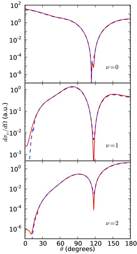
Figure 1: (color online) Differential cross section for electrons absorbing 0 (top) to 2 (bottom) photons. The solid red line is the cross section found with the Floquet $R$ matrix calculation, and the dashed blue line is calulated using the Kroll Watson approximation. This calculation was performed with the $R$ matrix boundary at 100 a.u., with 19 total Floquet channels and angular momentum channels up to $l=150$.

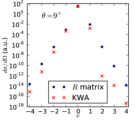
Figure 2: (color online) Differential cross sections at 9 degrees versus the number $\nu$ of photon energies gained by the electron. The cross section found via the $R$ matrix calculation (blue dots) has comparable order of magnitude to the Kroll Watson approximation (red crosses) for a few photon numbers, and it is several orders of magnitude smaller than the experimental results for all nonzero $\nu$. The parameters of the calculation are the same as for figure 1.

Note that the Floquet $R$ matrix calculation and the KWA agree very well for all but very small scattering angles. The zero photon cross section is also quite close to the experimental elastic electron argon cross section found by Furst et al. (1989), as expected. Figure 2 shows the differential cross section at 9 degrees for absorption and emission of up to 4 photons, again compared with the KWA result. Note that though they do not agree exactly, they differ with far fewer orders of magnitude than measured by Wallbank and Holmes at this scattering angle. For example, the differential cross sections they found for exchanges of 1 and 2 photons were on the order of 1 percent of the field free elastic differential cross section, while our calulations show these as roughly $10^{-2}$ percent and $10^{-6}$ percent respectively.

Differential cross sections calculated with $R$ matrix boundaries from 10 a.u. to 100 a.u. show no differences that are distinguishable from the convergence with respect to the basis. Our differential cross section also agrees with that of Chen and Robicheaux (1996), who used a variable gauge approach and chose an $R$ matrix boundary of 30 a.u. We can, therefore, rule out the possibility that the long range induced-dipole potential would yield the sort of diffraction suggested by Jaroń and Kamiński (1999) over distances comparable to or even several times the electron de Broglie wavelength.

It has been suggested that uncertainty in the scattering angle could account for higher observed cross sections. Madsen Madsen and Taulbjerg (1995) even suggests that the incoming electron beam is poorly collimated, leading to an effective error in the scattering angle as high as $8^{\circ}$, as opposed to the $2^{\circ}$ reported from the detector width Wallbank and Holmes (1994b). Convolving the cross sections shown in figure 1 with a gaussian having a width up to $8^{\circ}$ does not give a significant difference in the 1- and 2-photon cross sections, however. Whatever the source of such an error, uncertanties in the scattering angle would not explain the experimental cross sections for this geometry.

Sun et al. (1998) calculate a cross section for one photon exchange that is quantitatively quite close to our result. Their result for two photon exchange is several orders of magnitude higher, however. This may be due to a convergence issue, as a group using a similar method for laser-assisted helium scattering at first found high cross sections Jaroń and Kamiński (1997), but later found better results that are closer to the KWA Garland et al. (2002).

V Conclusions

The Floquet $R$ matrix method provides an exact solution of the Scrödinger equation in the velocity gauge. By comparing cross sections calculated with $R$ matrix boundaries up to 100 a.u., over ten times the de Broglie wavelength of a 10 eV electron, we have shown that the induced dipole potential for argon does not contribute to the laser assisted cross section. This is true even at small angles where the momentum transfer has a very small component along the field, and so the KWA is less valid. Diffraction from this long range piece of the potential can not account for the high cross sections found in the experiments of Wallbank and Holmes, which are several orders of magnitude higher than both the approximation and our calculations.

The most plausible explanation for the experimental results remains multiple scattering. Later experiments for helium by the same group claim to see the same high cross sections even when the gas is too dilute for multiple scattering to play a significant role Wallbank and Holmes (2001), so it is unclear whether this is the correct explanation. To our knowledge, a similar experiment for argon including characterization of the gas density has not been performed.

Discussions with A. Jaron-Becker and M. Tarana are much appreciated. We gratefully acknowledge the support of the Department of Energy, Office of Science.

References

- Kroll and Watson (1973) N. M. Kroll and K. M. Watson, Phys. Rev. A 8, 804 (1973).
- Wallbank and Holmes (1993) B. Wallbank and J. K. Holmes, Phys. Rev. A 48, R2515 (1993).
- Wallbank and Holmes (1994a) B. Wallbank and J. K. Holmes, J. Phys. B 27, 1221 (1994a).
- Wallbank and Holmes (1994b) B. Wallbank and J. K. Holmes, J. Phys. B 27, 5405 (1994b).
- Rabadán et al. (1994) I. Rabadán, L. Méndez, and A. S. Dickinson, J. Phys. B 27, L535 (1994).
- Geltman (1995) S. Geltman, Phys. Rev. A 51, R34 (1995).
- Varró and Ehlotzky (1995) S. Varró and F. Ehlotzky, Phys. Lett. 203, 203 (1995).
- Rabadán et al. (1996) I. Rabadán, L. Méndez, and A. S. Dickinson, J. Phys. B 29, L801 (1996).