Surface Code Threshold in the Presence of Correlated Errors

Abstract

We study the fidelity of the surface code in the presence of correlated errors induced by the coupling of physical qubits to a bosonic environment. By mapping the time evolution of the system after one quantum error correction cycle onto a statistical spin model, we show that the existence of an error threshold is related to the appearance of an order-disorder phase transition in the statistical model in the thermodynamic limit. This allows us to relate the error threshold to bath parameters and to the spatial range of the correlated errors.

The surface code is considered one of the best quantum error correction (QEC) codes to implement on physical devices DKP2002 ; DiVincenzo09-a ; YWC+12 . This stems from two major points: First, all syndromes and operations can be performed with spatially local operators; second, all threshold estimates show that, for sufficiently large lattices, the error threshold is the highest known for two-dimensional architectures with only nearest-neighbor interactions RH07 ; FWH11 ; bombin12 .

The error threshold is usually defined for stochastic error models. By assuming that errors are independent events and assigning a probability $p$ to each of these events, it has been shown numerically that the quantum information encoded in the surface can be faithfully protected when $p$ is below a critical value. Although this result is firmly established numerically, there are two big open questions that still need to be addressed. First, stochastic error models are approximations to reality that sometimes cannot be justified. In fact, most studies so far lacked a microscopic description of the interaction between physical qubits and the environment. Second, the same locality of operations and syndromes that makes the surface code powerful also makes it more susceptible to correlated errors. Thus, a discussion of the tradeoff between locality of operations and correlated errors is long overdue. In this Letter, we address both issues by employing a more realistic error model. We consider a Caldeira-Leggett type of environment where freely propagating bosonic modes couple linearly and locally to the physical qubits. Such a model has a very strong physical motivation since in most experimental implementations photons and phonons couple to the two-level systems making up the physical qubits. This model also plays a fundamental role in our understanding of decoherence Unruh:1995:992 and its interplay with QEC Novais:2006:040501 ; Novais:2007:040501 ; Novais2008 ; Ng:0810.4953v1 ; NERM10 ; Preskill.2012 .

Consider a logical qubit in a quantum memory. In a QEC cycle, the logical qubit is prepared and left to freely evolve during a certain time interval. Then, syndromes are extracted, and, if necessary, suitable error correction operations are implemented to bring the logical qubit back to its original state. In our analysis, we evaluate the fidelity of a logical qubit after such a QEC cycle under the assumption of nonerror syndromes. This assumption is not essential to our results, but makes the calculation more concise. In addition, we assume that the bath is initially at zero temperature and that it is reset to this temperature at the end of the QEC cycle.

Our results show a sharp transition between two distinct noise regimes. On one hand, below a fictitious critical temperature (which is related to microscopic parameters of the bath), the dissipation due to the bath cannot be suppressed by the encoding. On the other hand, above this critical temperature, we show that if the thermodynamic limit is taken, the effects of the bosonic environment become irrelevant and the logical qubit is fully protected.

Even though this investigation focuses on quantum information protection, the physical problem we consider has a much broader appeal. In essence, it amounts to a lattice gauge system interacting with a scalar bosonic field in two dimensions Kogut . In this language, the nonexistence of a quantum error threshold can be understood as the lifting of the ground state topological degeneracy. Our discussion of the error threshold can therefore be recast as a quantum phase transition. This fits into our earlier discussion of the threshold theorem as resembling a quantum phase transition Novais:2007:040501 . This analogy is nontrivial since the error threshold is in essence a driven dynamical problem, far from the equilibrium conditions required to describe phase transitions in statistical mechanics. This work turns what was an analogy into a well-defined map. Therefore, we believe that the results presented here transcend our original motivation and complement the recent discussion in Ref. Preskill.2012, .

The model –We consider physical qubits $\{\vec{\sigma}_{i}\}_{i=1,\ldots,N}$ (i.e., spin 1/2 systems) located on the links of a square lattice with open boundary conditions (see Fig. 1). The QEC code is defined by an encoding prescription and a set of stabilizer operators Gottesman . The stabilizer operators of the surface code are easily labeled when we define stars and plaquette operators. Star operators are the product of the four $\sigma^{x}$ operators of qubits adjacent to a vertex of the square lattice, $A_{\Diamond}=\prod_{i\in\diamondsuit}\sigma_{i}^{x}$. Similarly, plaquette operators are the product of four $\sigma^{z}$ of qubits located at the edges of a tile of the square lattice, $B_{\square}=\prod_{i\in\square}\sigma_{i}^{z}$. Each plaquette and star is a stabilizer that has to be measured at the end of a QEC period. The logical operators are defined as $\bar{X}=\prod_{i\in\Gamma}\sigma_{i}^{x}$, where $\Gamma$ is a path along the center of the plaquettes crossing horizontally the lattice, and $\bar{Z}=\prod_{i\in\bar{\Gamma}}\sigma_{i}^{z}$, where $\bar{\Gamma}$ is a path along the edge of the plaquettes crossing the lattice vertically. Finally, the codewords of the surface code are also easily written:

$$\left\{|\bar{\uparrow}\rangle=G|F_{z}\rangle,|\bar{\downarrow}\rangle=\bar{X}|\bar{\uparrow}\rangle\right\},$$ (1)

where $G=\frac{1}{\sqrt{2^{N_{A}}}}\prod_{\diamondsuit}\left(1+A_{\diamondsuit}\right)$, $N_{A}$ is the total number of possible stars, and $|F_{z}\rangle$ is the ferromagnetic state along the positive $z$ direction, namely, $|F_{z}\rangle=\prod_{i=1}^{N}|\uparrow\rangle_{i,z}$.

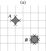
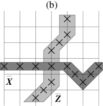
Figure 1: (a) Star ($A$) and plaquette ($B$) operators. (b) Examples of logical $\bar{X}$ and $\bar{Z}$ operators. The crosses and shades indicate the qubits involved in the respective operator.

The Hamiltonian we consider is written as

$$H=H_{0}+V,$$ (2)

where $H_{0}$ is a free bosonic Hamiltonian, $H_{0}=\sum_{\bf k\neq 0}\,\omega_{\bf k}a_{\bf k}^{\dagger}a_{\bf k}$, and $V=\frac{\lambda}{2}\sum_{\bf r}f({\bf r})\sigma_{\bf r}^{x}$, where ${\bf r}$ denotes the spatial location of a qubit and $f$ is a local bosonic operator,

$$f({\bf r})=\frac{\omega_{0}}{L^{D}}\sum_{{\bf k}\neq 0}\left|{\bf k}\right|^{s}\left(e^{i{\bf k}\cdot{\bf r}}a_{\bf k}^{\dagger}+e^{-i{\bf k}\cdot{\bf r}}a_{\bf k}\right).$$ (3)

Here, $D$ is the bath spatial dimension, $\omega_{\bf k}=v|{\bf k}|$, and $\omega_{0}$ is a microscopic coupling that makes $f$ dimensionless (we adopt units such that $\hbar=1$). This error model leads to a remarkably simple evolution operator in the interaction picture: For a time interval $\Delta$, with the environment starting at its ground state, we have NERM10

$$\hat{U}(\Delta) = e^{-\frac{\lambda^{2}}{2}N{\cal G}_{\bf rr}(\Delta)}\,e^{-\frac{\lambda^{2}}{2}\sum_{{\bf r}\neq{\bf s}}\Phi_{{\bf r}{\bf s}}(\Delta)\sigma_{\bf r}^{x}\sigma_{\bf s}^{x}}$$ (4)

$$\times\ :e^{-i\lambda\sum_{\bf r}F_{\bf r}(\Delta)\sigma_{\bf r}^{x}}:,$$

where $N$ is the total number of qubits, ${\cal G}_{{\bf r}{\bf s}}(\Delta)=\langle 0|F_{\bf r}(\Delta)\,F_{\bf s}(\Delta)|0\rangle$, $F_{\bf r}(\Delta)=\int_{0}^{\Delta}dt\,f({\bf r},t)$, $\Phi_{{\bf r}{\bf s}}(\Delta)={\cal G}_{{\bf r}{\bf s}}(\Delta)+\int_{0}^{\Delta}dt_{1}\int_{0}^{t_{1}}dt_{2}\left[f({\bf r},t_{1}),f({\bf s},t_{2})\right]$, and $::$ stands for normal ordering. For Ohmic baths, the correlation function for ${\bf r}\neq{\bf s}$ takes the simple form bathcorrelator

$$\Phi_{{\bf r}{\bf s}}(\Delta)=\left(\frac{\omega_{0}}{v}\right)^{2}\left\{\begin{array}[]{ll}\mbox{arcsh}\left(\frac{v\Delta}{|{\bf r}-{\bf s}|}\right)+\frac{i\pi}{2},&0<|{\bf r}-{\bf s}|<v\Delta,\\ i\,\mbox{arcsin}\left(\frac{v\Delta}{|{\bf r}-{\bf s}|}\right),&0<v\Delta<|{\bf r}-{\bf s}|.\end{array}\right.$$ (5)

Thus, we can introduce a fictitious inverse temperature $\beta=\frac{1}{2}\left(\frac{\lambda\omega_{0}}{v}\right)^{2}$ and rewrite the intermediate factor that contains the two-spin interaction in Eq. (4) as $e^{-\beta\sum_{{\bf r}\neq{\bf s}}J_{{\bf r}{\bf s}}\,\sigma_{\bf r}^{x}\sigma_{\bf s}^{x}}$, where $J_{{\bf r}{\bf s}}$ represents an effective antiferromagnetic coupling comment1 .

To simplify the notation, we assume that the system is prepared initially in the logical state $|\bar{\uparrow}\rangle$ and the boson field initial state is the vacuum

$$|\psi_{0}\rangle=(G|F_{z}\rangle)\otimes|0\rangle.$$ (6)

We then let the system evolve under the Hamiltonian $H$ until a time $\Delta$, when an error correction protocol is performed flawlessly.

The assumptions –Since we are only allowing for bit-flip errors, the syndrome outcome for the star stabilizers is trivial. For the plaquettes, in principle, all possible syndromes should be considered. However, it is useful to look at the most benign evolution and assume that all plaquette syndromes return a nonerror. This nonerror syndrome provides an upper bound to the available computational time and also substantially simplifies the calculation since it removes from consideration which recovery operation should be performed to steer the system back to the computational basis.

In QEC theory, it is standard to focus only on the qubit system’s evolution and disregard any change to the environment’s state, even though the latter is a also a quantum system capable of sustaining correlations. If no extra step is taken to dissipate those correlations, the environment will keep a memory of events that happened between the QEC periods. Keeping track of such bath-induced, long-time correlations between QEC cycles in a fidelity calculation is a difficult task even for simple, nontopological logical qubit systems Novais2008 ; NERM10 . Thus, to proceed with the calculation, we consider an extra step to the QEC protocol. In addition to projecting the quantum computer wave function back to the logical Hilbert space, we assume that at the end of the QEC step the environment is reset to its ground state. Hence, from this point on, we are excluding from the calculation any spatial correlation between QEC periods, as well as memory and spatial correlations between the time evolution of bras and kets. Physically, this is equivalent to assuming that the environment thermalizes with an even larger zero-temperature bath during the QEC period. When we adopt this extra simplifying assumption, we can conveniently rewrite the nonerror syndrome projector as

$$P^{\prime}=|\psi_{0}\rangle\langle\psi_{0}|+\bar{X}|\psi_{0}\rangle\langle\psi_{0}|\bar{X}.$$ (7)

By using Eq. (7), it becomes now straightforward to write an expression for the logical qubit fidelity just after the syndrome extraction:

$${\cal F} = \frac{|{\cal A}|}{\sqrt{|{\cal A}|^{2}+|{\cal B}|^{2}}},$$ (8)

where ${\cal A}=\langle\psi_{0}|\hat{U}(\Delta)|\psi_{0}\rangle$ and ${\cal B}=\langle\psi_{0}|\bar{X}\hat{U}(\Delta)|\psi_{0}\rangle$.

Fidelity calculation –Thus, our task now is reduced to evaluate ${\cal A}$ and ${\cal B}$. By using Eq. (4), it is straightforward to show that

$${\cal A}=\chi\left\langle F_{z}\left|e^{-\beta{\cal H}}G^{2}\right|F_{z}\right\rangle\\$$ (9)

and

$${\cal B}=\chi\left\langle F_{z}\left|\bar{X}e^{-\beta{\cal H}}G^{2}\right|F_{z}\right\rangle\\$$ (10)

where

$${\cal H}=\sum_{{\bf r}\neq{\bf s}}J_{{\bf r}{\bf s}}\,\sigma_{\bf r}^{x}\sigma_{\bf s}^{x},$$ (11)

and $\chi=e^{-\frac{\lambda^{2}}{2}N{\cal G}_{\bf rr}(\Delta)}$. Notice that although we chose to start with a microscopic model of the environment to make a connection to physical implementations, we could as well have started by imposing an effective two-body interaction between qubits such as that defined by ${\cal H}$.

Clearly, when $\beta\to 0$, we have ${\cal B}\to 0$ and ${\cal F}\to 1$. A perturbative expansion for small $\beta$ is the standard route to discuss the error threshold. This “high-temperature” expansion will be discussed elsewhere. Here we follow a different route. To understand the opposite limit $\beta\to\infty$, we need to rewrite $|F_{z}\rangle$ in the $x$ basis:

$$|F_{z}\rangle=\prod_{i=1}^{N}\left(\frac{\left|\uparrow\right\rangle_{i,x}+\left|\downarrow\right\rangle_{i,x}}{\sqrt{2}}\right).$$ (12)

This dual representation corresponds to a “low-temperature” expansion, and it is suitable for describing the regime where error correlations are strong. Inserting Eq. (12) into (9) and (10), we obtain

$${\cal A} = \frac{\chi}{2^{N}}\sum_{S}e^{-\beta E_{s}}\langle S|G^{2}|S\rangle,$$ (13)

$${\cal B} = \frac{\chi}{2^{N}}\sum_{S}e^{-\beta E_{s}}\langle S|\bar{X}G^{2}|S\rangle,$$ (14)

respectively, where $|S\rangle$ is an element of the $x$ basis and $E_{s}=\langle S|{\cal H}|S\rangle$ is its “energy”. Notice that $E_{s}$ may have an imaginary part.

If we had unrestricted sums in Eqs. (13) and (14), we would be essentially discussing a two-dimensional Ising model. However, $G^{2}$ projects $|S\rangle$ onto the subspace of positive stars and, among other things, removes time reversal state of $\left|S_{\pm}^{\gamma}\right\rangle$ from the sum. This restriction makes the computation of ${\cal A}$ and ${\cal B}$ nonstandard. Nevertheless, the action of $\bar{X}$ is to introduce a sign between two distinct classes of states. To better understand this, we need a more convenient way to write the states $|S\rangle$ in the restricted subspace of positive stars. It is not hard to prove that these states fall into two groups, $\{|S_{+}\rangle\}$ and $\{|S_{-}\rangle\}$, where

$$|S_{+}\rangle=\prod_{j}B_{\square_{j}}|F_{x}\rangle\qquad\mbox{and}\qquad|S_{-}\rangle=\bar{Z}_{\gamma}|S_{+}\rangle.$$ (15)

(See Fig. 2.) Here, $\prod_{j}B_{\square_{j}}$ is a product of plaquettes that do not touch a logical error $\bar{Z}_{\gamma}$ and $|F_{x}\rangle$ is the ferromagnetic state in the $x$ basis. Splitting the terms of the sums in Eqs. (13) and (14) between these two groups of states, we rewrite ${\cal A}=\frac{\chi}{2^{N}}({\cal T}_{+}+{\cal T}_{-})$ and ${\cal B}=\frac{\chi}{2^{N}}({\cal T}_{+}-{\cal T}_{-})$, where

$${\cal T}_{\pm}=\sum_{S_{\pm}}\left\langle S_{\pm}\left|e^{-\beta{\cal H}}\right|S_{\pm}\right\rangle.$$ (16)

Thus, we have to evaluate the “free energies” of the two groups of states (see Fig. 2).

The double sum in ${\cal H}$ [see Eq. (11)] runs over lattice points ${\bf r}$ and ${\bf s}$ inside and outside the path of the logical operator $\bar{Z}_{\gamma}$. Thus, let us break these points into two sets, namely, $\{{\bf r}\}=\{{\bf t}_{\gamma}\}\oplus\{{\bf u}_{\gamma}\}$ and $\{{\bf s}\}=\{{\bf v}_{\gamma}\}\oplus\{{\bf w}_{\gamma}\}$, where ${\bf t}_{\gamma}$ and ${\bf v}_{\gamma}$ belong to $\bar{Z}_{\gamma}$ while ${\bf u}_{\gamma}$ and ${\bf w}_{\gamma}$ do not. Furthermore, let us factor the sum over all $S_{+}$ into a sum over paths $\gamma$ and a sum over configurations $S_{+}^{\gamma}$ compatible with a logical operator along this path, namely, $\sum_{S_{\pm}}=\sum_{\gamma}\sum_{S_{\pm}^{\gamma}}$. After some simple algebra, we obtain ${\cal T}_{\pm}=\sum_{\gamma}e^{-\beta\epsilon_{\gamma}}\sum_{S_{\pm}^{\gamma}}z^{\gamma}_{\pm}$, where $\epsilon_{\gamma}=\left\langle S_{\pm}^{\gamma}\left|\sum_{{\bf t}{\bf v}}\,J_{{\bf t}{\bf v}}\,\sigma_{\bf t}^{x}\sigma_{\bf v}^{x}\right|S_{\pm}^{\gamma}\right\rangle$ and

$$z^{\gamma}_{\pm}=\left\langle S_{+}^{\gamma}\left|e^{-\beta\sum_{{\bf u}\neq{\bf w}}J_{{\bf u}{\bf w}}\,\sigma_{\bf u}^{x}\sigma_{\bf w}^{x}\mp\beta\sum_{\bf w}h_{\bf w}^{\gamma}\,\sigma_{\bf w}^{x}}\right|S_{+}^{\gamma}\right\rangle,$$ (17)

with $h_{\bf w}^{\gamma}=\sum_{\bf t}J_{{\bf t}{\bf w}}$. We can see that the effect of the logical operator $\bar{Z}_{\gamma}$ is to introduce a boundary term represented by the effective local magnetic field $h_{\bf w}^{\gamma}$.

We are now in the position to state our definition of the quantum error threshold. We define the critical parameter $\beta_{c}$ as the value of $\beta$ that separates the regime where ${\cal F}=1$ from the regime where ${\cal F}<1$ in the thermodynamic limit ($N\rightarrow\infty$).

Phase transition –The evaluation of $z^{\gamma}_{\pm}$ in Eq. (17) is a formidable task, and a general answer may only be achievable through numerical simulations. Hence, we now restrict our considerations to more manageable effective qubit interactions. Let us first consider the case of

$$J_{{\bf r}{\bf s}}=\begin{cases}J,&{\bf r},{\bf s}\ \mbox{nearest neighbors},\\ 0&\mbox{otherwise},\end{cases}$$ (18)

where $J$ is real. Such a case is of physical relevance. Any measurement or operation on the plaquettes and stars can introduce short-range correlated errors, regardless of the presence of an environmental bath. For an Ohmic bath, it corresponds to set $v\Delta$ to the order of the lattice spacing.

To show that an order-to-disorder transition indeed exists, let us consider Eq. (17) with (18) in the absence of the field $h_{\bf w}^{\gamma}$. Using Eq. (15), we obtain

$$z_{S_{\pm}^{\gamma}}=\left\langle F_{x}\left|\prod_{j}B_{\square_{j}}e^{\beta\sum_{{\bf u}\neq{\bf w}}J_{{\bf u}{\bf w}}\,\sigma_{\bf u}^{x}\sigma_{\bf w}^{x}}\prod_{j}B_{\square_{j}}\right|F_{x}\right\rangle,$$ (19)

where we have multiplied all spins in one of the sublattices by $-1$ to make the model ferromagnetic. The products over plaquettes introduce a sum over loops where the qubits at these these loops have negative eigenvalues (they are located at the edges of the shaded regions in Fig. 2). Let us label these qubits by ${\bf a}$ and ${\bf b}$ and use ${\bf c}$ and ${\bf d}$ to label qubits with positive eigenvalues. Thus

$$z_{S_{\pm}^{\gamma}}=e^{\beta\sum_{{\bf a}\neq{\bf b}}J_{{\bf a}{\bf b}}}\,e^{\beta\sum_{{\bf c}\neq{\bf d}}J_{{\bf c}{\bf d}}}\,e^{-\beta\sum_{{\bf a}\neq{\bf c}}J_{{\bf a}{\bf c}}}.$$ (20)

At low fictitious temperatures, the first two factors in Eq. (20) dominate. The third factor leads to excitations above the ferromagnetic ground state whose energy is $E_{F}$. Therefore, we can go back Eq. (17) and write (for $h_{\bf w}^{\gamma}=0$)

$$\sum_{S_{\pm}^{\gamma}}z^{\gamma}=e^{\beta E_{F}}\left(1+\sum_{\rm loops}e^{-2\beta\sum_{{\bf a}\in{\rm loop},{\bf c}\notin{\rm loop}}J_{{\bf a}{\bf c}}}\right).$$ (21)

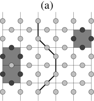
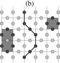
Figure 2: Example of states that contribute to the $S_{+}$ (a) and $S_{-}$ (b) sums [see Eq. (15)]. The light (dark) circles indicate qubits in $+$ ($-$) $\sigma^{x}$ eigenstates. The dark line indicates the path of the logical error $\bar{Z}_{\gamma}$, which is active in (b) and inactive in (a).

Then, the energy cost of a loop with length $\ell$ is equal to $4J\ell$. The scaling of the number of loops with $\ell$ is well known: $N_{\ell}\sim\mu^{\ell}$, where $\mu$ is the lattice connectivity constant (e.g., $\mu\approx 2.638$ for a square lattice) connectivity . Hence, the contribution of loops with length $\ell$ to $\sum_{S_{\pm}^{\gamma}}z^{\gamma}$ goes as $\mu^{\ell}\,e^{-8\beta J\ell}$. Clearly, a tradeoff between energy minimization and “entropy” maximization takes place, and a phase transition is expected at $\beta=\beta_{c}$, where

$$\beta_{c}\approx\frac{\ln\mu}{8J}.$$ (22)

For $\beta>\beta_{c}$ the system is in its ordered phase. Thus, we expect the system to be sensible to the boundary magnetic field direction, leading to ${\cal F}<1$ after the QEC period. In particular, there is an obvious result to be stated. At the zero temperature limit $\beta\to\infty$, only the “ground state” contributes to the sums (i.e., only the ${\cal T}_{-}$ sum survives). Hence, $|{\cal A}|=|{\cal B}|$ and ${\cal F}=\frac{1}{2}$. Conversely, for $\beta<\beta_{c}$ (therefore $\lambda<\lambda_{c}$), a disordered phase develops, leading to the insensibility to the boundary field and, therefore, ${\cal F}=1$.

There are some roadblocks to studying the general case represented by the correlator in Eq. (5). The first one is its imaginary part. It is expected that any imaginary part would have a negative effect on the fidelity (a conclusion that can be reached by applying the Schwarz inequality). Even if we disregard this imaginary part, the magnetic model given by the real part of Eq. (5) may lead to frustration. However, since the real part of the correlator is a slow growing function, it is likely that the model is controlled by boundary effects (as many other features of topological systems are). Only through future numerical work will it be possible do address these issues.

In order to gain some insight into the effects of long-range correlations, we arbitrate a stripped version of the Ohmic model. Consider the case where qubits on one of the sublattices interact only with qubits on the other sublattice through the real part of Eq. (5). This interaction preserves the bipartite nature of the lattice and we can again map it onto a ferromagnetic model. We can repeat all steps of the calculation done in the case with nearest-neighbor interactions. Then, the energy cost of a loop with length $\ell$ is equal to $(n-2)J\ell$, where $n$ is the number of sites connected to any lattice site through the interaction (i.e., $n$ is related to the range of the interaction). The transition happens at

$$\beta_{c}\approx\frac{\ln\mu}{nJ}.$$ (23)

Note that $\beta_{c}$ explicitly depends on the interaction range. In a strict sense, if all qubits in the lattice are in the “causality cone” (and therefore participate in ${\cal H}$), there is never a threshold. Although this could seem a dismal result, it also shows us that a finite QEC period introduces an infrared cutoff that creates a finite transition temperature. The smallest of such transition temperatures corresponds to the case of nearest neighbors, Eq. (18). Finally, we note that, under the same assumptions that we used for the Ohmic bath, super-Ohmic environments are local and therefore will always yield a finite transition “temperature”. Conversely, sub-Ohmic baths will require an infrared cutoff to yield a finite threshold.

In conclusion, in this Letter we studied the fidelity of a logical qubit encoded with the surface code after one complete QEC period. We derived a nontrivial mapping to a statistical mechanical problem and provided an analytical expression for the error threshold for some correlated models. This mapping provides a promising route for exploring fault tolerance of topological quantum error correction codes in the presence of realistic environments.

We thank M. Correa and R. Paszko for helpful discussions and C. Chamon and R. Raussendorf for insightful comments. E.N. was partially supported by INCT-IQ and CNPq (Brazil). E.R.M. was supported in part by the ONR and NSF (USA).

References

- (1) E. Dennis, A. Kitaev, A. Landahl, and J. Preskill, J. Math. Phys. (N.Y.) 43, 4452 (2002).
- (2) D. P. DiVincenzo, Phys. Scri. T 137, 014020 (2009).
- (3) X.-C. Yao et al., Nature (London) 482, 489 (2012).
- (4) R. Raussendorf and J. Harrington, Phys. Rev. Lett. 98, 190504 (2007).
- (5) A. G. Fowler, D. S. Wang, and L. C. L. Hollenberg, Quantum Inf. Comput. 11, 8 (2011).
- (6) H. Bombin, R. S. Andrist, M. Ohzeki, H. G. Katzgraber, and M. A. Martin-Delgado, Phys. Rev. X 2, 021004 (2012).
- (7) W. G. Unruh, Phys. Rev. A 51, 992 (1995).
- (8) E. Novais and H. U. Baranger, Phys. Rev. Lett. 97, 040501 (2006).
- (9) E. Novais, E. R. Mucciolo, and H. U. Baranger, Phys. Rev. Lett. 98, 040501 (2007).
- (10) E. Novais, E. R. Mucciolo, and H. U. Baranger, Phys. Rev. A [78 012314 (2008).
- (11) H. K. Ng and J. Preskill, Phys. Rev. A 79, 032318 (2009).
- (12) E. Novais, E. R. Mucciolo, and H. U. Baranger, Phys. Rev. A 82, 020303(R) (2010).
- (13) J. Preskill, technical report No. CALT 68-2881, 2012; arXiv:1207.6131.
- (14) J. Kogut, Rev. Mod. Phys. 51, 659 (1979).
- (15) D. Gottesman, Phys. Rev. A 54, 1862 (1996); A. R. Calderbank, E. M. Rains, P. W. Shor, and N. J. A. Sloane, Phys. Rev. Lett. 78, 405 (1997).
- (16) D. López, E. R. Mucciolo, and E. Novais (in preparation).
- (17) When the initial state of the environment is a thermal state, a thermal length , added to the bosonic propagator of Eq. (4), causes correlation functions to decay exponentially over distances larger than . Such a situation can be readily included in the effective model of Eq. (11)
- (18) N. Madras and G. Slade, The Self-Avoiding Walk (Birkhäuser, Boston, 1996).