X-ray spectroscopy and monitoring of Novae††thanks: Using data obtained with XMM-Newton (an ESA science mission with instruments and contributions directly funded by ESA Member States and NASA), Chandra, and Swift–X-ray spectroscopy and monitoring of Novae††thanks: Using data obtained with XMM-Newton (an ESA science mission with instruments and contributions directly funded by ESA Member States and NASA), Chandra, and Swift
X-ray spectroscopy and monitoring of Novae††thanks: Using data obtained with XMM-Newton (an ESA science mission with instruments and contributions directly funded by ESA Member States and NASA), Chandra, and Swift
Abstract
The 21st century X-ray observatories XMM-Newton, Chandra, and Swift
gave us completely new insights into the X-ray behaviour of
nova outbursts. These new-generation X-ray observatories provide
particularly high spectral resolution and high density in
monitoring campaigns, simultaneously in X-rays and UV/optical.
The entire evolution of several nova outbursts has been observed
with the Swift XRT and UVOT instruments, allowing studies of the
gradual shift of the peak of the SED from UV to X-rays, time
scales to the onset and duration of the X-ray brightest supersoft
source (SSS) phase, and pre- and post-SSS X-ray emission.
In addition, XMM-Newton and Chandra observations can efficiently
be scheduled, allowing deeper studies of strategically chosen
evolutionary stages. Before Swift joined in 2005, Chandra and
XMM-Newton blind shots in search of SSS emission unavoidably
led to some underexposed observations taken before and/or after the SSS
phase. More systematic Swift studies reduced this number while
increasing the number of novae.
Pre- and post-SSS spectra at low and high spectral resolution
were successfully modelled with collisional plasma models.
Pre-SSS emission arises in shocks and post-SSS emission
in radiatively cooling thin ejecta. In contrast, the grating
spectra taken during the SSS phase are a lot more complex than
expected and have not yet been successfully modeled.
Available hot WD radiation transport models give
only approximate reproduction of the observations, and make
some critical assumptions that are only valid in isolated
WDs. More grating spectra which would be important to search
for systematic trends between SSS spectra and system parameters.
Summary of well-established discoveries with Swift, XMM-Newton, and Chandra:
About 50% of novae display faint X-ray emission
before the start of the SSS phase
The start of the SSS phase is not a smooth process. High-amplitude
variations during the early SSS phase were seen that disappear
close to the time when the optical plateau phase begins.
The end of the SSS phase is in most cases a smooth process.
The SSS grating spectra contain continuum spectra that
roughly resemble a blackbody shape
The SSS X-ray grating spectra of systems with known high inclination angles contain emission lines on top of the continuum
The SSS X-ray spectra of systems with unknown or low inclination
angles contain deep absorption lines from the interstellar medium and
local, high-ionisation absorption lines that are blue shifted.
keywords:
novae, cataclysmic variables – stars: individual (RS Oph) – stars: individual (V4743 Sgr) – stars: individual (V382 Vel) – stars: individual (V458 Vul) – stars: individual (V2491 Cyg) – stars: individual (V723 Cas) – stars: individual (U Sco) – stars: individual (V1494 Aql)1 Introduction
Classical Novae (CNe) occur in cataclysmic binary systems (CVs) in which
the close companion star provides H-rich nuclear burning fuel that is
transferred to the surface of the white dwarf (WD) primary via accretion.
Once enough hydrogen-rich
material is accumulated, a thermonuclear runaway triggers the initial
explosion. The radiative energy output exceeds the Eddington limit and
drives an optically thick wind. The way we observe a nova from Earth
depends on the properties of the ejected material.
Absorption and scattering change the colour of the light that
originates from the central nuclear burning processes. During radiative
transport through the optically thick part of the ejecta, the peak of the
broad-band spectrum (or spectral energy distribution, SED), is
shifted to successively lower energy. Observed optical light arises
after radiation transport through a larger column than X-ray
emission. The opacity evolution of the
ejecta may or may not be a homogeneous process, but the bolometric
luminosity should be dictated by the energy budget of central nuclear
burning that is believed to be constant until all hydrogen burning material
has been consumed or ejected (Gallagher & Starrfield 1976). With the continuously shifting SED,
observations of nova evolution require multiwavelength monitoring,
including the UV and X-ray bands. The last evolutionary phase before a
nova turns off is the supersoft source (SSS) phase, during which
atmospheric X-ray emission from the central regions of the ejecta,
close to the surface of the WD, can be observed. The start of the
SSS phase depends on the opacity evolution of the ejecta and can not
be predicted accurately. Before and after the SSS phase, novae are
X-ray faint, and scheduling X-ray observations yields a risk of
non-detections if observed too early or too late. Recent dense
X-ray/UV monitoring observations obtained with the Swift satellite
give important insights into the long-term opacity evolution of the
ejecta, also facilitating more accurate scheduling of deeper X-ray
observations, employing the grating spectrometers on board
XMM-Newton and Chandra. X-ray grating spectra yield higher
spectral resolution, allowing determinations of physical
properties such as the energetics of nuclear burning, mass of the
underlying WD, and chemical composition. Followup X-ray observations
are also of longer continuous durations, allowing studies of
short-term ( s) variability and associated spectral changes.
In this review, I summarise observing strategies to catch the SSS phase, at first via educated guesses based on theoretical expectations and observational evidence from optical (Sect. 4.2), and later assisted with Swift monitoring observations (Sect. 4.3). I only touch on some selected nova observations to exemplify the key points of observing strategies and data analysis. More general conclusions from the entirety of all observations are presented in Sect. 5.
2 A brief history of past X-ray observations of novae
Before the advent of Chandra and XMM-Newton, instruments of
moderate sensitivity and spectral resolution but large fields
of view were available. In surveys of the Large Magellanic
Cloud (LMC) with the Einstein Observatory, a few mysterious
luminous sources with extremely soft spectra were discovered
(Long, Helfand, &
Grabelsky 1981) which were later combined in a new
class of Super Soft Sources (SSS) after more had been discovered
with ROSAT (Kahabka, Pietsch, &
Hasinger 1994; Greiner, Hasinger, &
Kahabka 1991). The underlying systems
were identified as accreting WDs with ongoing
nuclear burning on their surface (Kahabka & van den Heuvel 1997). Since novae
occur in such systems, the concept of constant bolometric
luminosity throughout the evolution with a continuous shift
of the peak of the SED towards higher energies, predicts that
they emit SSS X-ray spectra during their late, X-ray bright,
phase (Gallagher & Starrfield 1976). This was confirmed by, e.g., EXOSAT and
ROSAT observations (Oegelman, Krautter, &
Beuermann 1987). Monitoring observations
over time intervals of 2-3 years resulted in rough light
curves that could be divided into a rise phase, plateau phase,
and decline phase (Krautter, Ögelman,
Starrfield, Wichmann, & Pfeffermann 1996).
The available X-ray detectors of the time allowed no precise
measurements of photon energies, leaving uncertainties of
several 10-100 eV. Nevertheless, the term ’X-ray spectrum’ is
occasionally used for 30-100 channel distributions of
photon energies. Obviously, no detailed spectral modelling is
possible with such data, and the first spectral characterisations
consisted of mere blackbody fits yielding effective temperatures
of several 10 eV (a few K) and bolometric luminosities
near or even beyond the Eddington limit (for electrons) of a
1-M⊙ WD. Such high values of luminosity, several months to
years after the initial outburst, imply an unphysically high total
mass loss. In light of the incorrect assumption of a blackbody model
(thermal equilibrium), the corresponding best-fit parameters
have no physical meaning.
In an attempt to derive more physically meaningful results,
atmosphere models were applied. For example,
Balman, Krautter, &
Ögelman (1998) determined a lower luminosity from LTE
atmosphere model fits. However, including
further more physics of non-LTE models, yield different
luminosities again, e.g., Hartmann & Heise (1997). When calling in
mind the small number of observed energy channels, one may
wonder whether atmosphere models with their high degree of
complexity are sufficiently constrained by the data.
The dilemma of the low-resolution spectra is that good fits
to the data can be achieved with either well-constrained but
unphysical models or with more physical but unconstrained models.
None of these approaches can lead us to truly informative results.
Substantially higher spectral resolution is undoubtedly needed,
and the Chandra and XMM-Newton missions with their grating
spectrometers (see Sect. 3.1) are a great leap
forward. This article concentrates on the Swift and XMM-Newton/Chandra
light curves and spectra. For more information on early X-ray
observations of novae, I refer to reviews by
Krautter (2002, 2008); Starrfield, Iliadis, &
Hix (2008); Bode & Evans (2008).
3 Current-day X-ray observing facilities
In the following subsections, the instrumentation of XMM-Newton, Chandra, and Swift is described in brevity.
3.1 XMM-Newton and Chandra
Chandra and XMM-Newton carry CCD spectrometers with similar energy
resolution of previous missions but with higher sensitivity and
spatial resolution. In addition, much higher spectral resolution
can be achieved with the new gratings. The dispersed photons are
recorded by X-ray sensitive detectors whose spatial resolution
determines the spectral resolution of the extracted spectrum.
XMM-Newton carries three X-ray mirrors with one
directing all light on a single pn CCD detector array
(Strüder et al. 2001) while the light from the other two mirrors
are shared between Metal Oxide Semi-conductor (MOS) detectors
(Turner et al. 2001) and Reflection Grating Spectrometers (RGS;
den Herder et al. 2001). The wavelength range of RGS1 and RGS2 is
6-38 Å, and the wavelength resolution is Å.
The Chandra mission carries two grating spectrometers,
a Low- and a High- Energy Transmission Grating (LETGS and HETGS),
covering the wavelength ranges 1-175 Å and 1-35 Å,
with wavelength resolutions of 0.06 and 0.01 Å, respectively.
As recording devices, a microchannel high-resolution image
(HRI) detector and chip arrays of the Advanced CCD Imaging
Spectrometer (ACIS) are available and can be combined depending
on scientific demands. The LETGS/HRC-S combination covers a wavelength
range from 1-175 Å at 0.06 Å resolution, and the HETGS/ACIS-S
combination covers 1-38 Å at 0.02 Å resolution. The LETGS/ACIS-S
combination (1-38 Å at 0.06 Å resolution) is sometimes used
for higher effective areas at 20-38 Å at the expense of spectral
resolution compared to HETGS/ACIS-S and wavelength coverage compared
to LETGS/HRC-S. The ACIS detector allows order sorting, thus the
removal of higher-dispersion order photons overlapping with first-order
photons, taking advantage of the energy resolution of the ACIS. The HRC has not
sufficient energy resolution for order sorting but suffers no
pileup. Order sorting is also possible with the XMM-Newton/RGS.
3.2 Swift /UV/X-ray Observatory
The primary purpose of Swift is to detect -ray bursts (GRB)
and carry out rapid follow up observations in the X-ray and UV bands.
The satellite was thus designed with extremely short slew times between
distant targets in the sky. The required instrumentation needs to be
sensitive from rays via X-rays, down to UV and
optical. A GRB detected by the Burst Alert Telescope (BAT) can then
be followed up with the X-Ray Telescope (XRT; Burrows et al. 2005) and
finally with Ultra-Violet/Optical Telescope (UVOT; Roming et al. 2005).
The XRT and UVOT resemble the Metal Oxide Semi-conductor (MOS) and
the Optical Monitor (OM) on board XMM-Newton, respectively.
The XRT allows a more precise
determination of the position of a GRB and rough spectral
parameters such as flux and neutral hydrogen column density,
. Deeper observations with more sensitive observatories
such as Chandra or XMM-Newton, but also by Suzaku, can be
planned, and adequate exposure times can be calculated.
Owing to it’s low-Earth orbit of minutes, Swift can
take no long, continuous observations. The maximum visibility
for the majority of targets is ks (depending on
declination). Deeper Swift observations
therefore consist of multiple short snapshots. Photometric
studies are only possible for variations on time scales of days
or on very short time scales of seconds to minutes.
Swift detects about 90 GRBs a year and spends some % of the available observing time for followups (Kim Page, priv. comm). More than half of the Swift time budget can be filled with observations of other targets. The low-Earth orbit allows only short snapshots of a few hundred seconds every 96 minutes, each yielding an X-ray and UV/optical flux plus some spectral information. While the resulting X-ray spectra can not compete against those obtained from long, uninterrupted Chandra or XMM-Newton observations, large series of Swift snapshots over extended periods of time are of high value to monitor the X-ray and UV evolution of variable sources such as supernovae, novae, and X-ray binaries, in unprecedented detail.
4 X-ray Observations of Novae
A large number of Swift, XMM-Newton, and Chandra observations of novae have been taken, not all of which can be discussed in this review. Early Swift observations focused on single detections of older novae, while a prolific monitoring program was developed after the initial monitoring of the prestigious recurrent nova RS Oph was extremely successful. Some examples are described in Sect. 4.1. Before these monitoring observations were done, XMM-Newton and Chandra had to dig in the mist to catch the important SSS phase with the X-ray gratings, which is described in Sect. 4.2. The time by which the SSS phase should start, and thus the best time for deep X-ray grating observations, is not well constrained by observations in other wavelength bands. For example, an indicator for the presence of SSS emission could be observations of high-ionisation optical lines (Schwarz et al. 2011). Swift-assisted grating observations are much more efficient, which is described in Sect. 4.3. I touch on individual novae, describing the respective observing strategies and some results from data analysis. Beyond the examples given here, there are a lot more, and for further reading, I recommend Schwarz et al. (2011). I focus on the spectral analysis with only brief mention of additional timing analysis.
4.1 Swift observations
The first Swift observations of novae addressed the question whether
or not any significant post-outburst emission was still present from
previous novae. For example, V1494 Aql (see Sect. 4.2)
was observed
three times, more than six years after outburst, and was not detected.
Meanwhile, V4743 Sgr that was observed four years after outburst,
yielded a clear detection. The old nova V723 Cas from 1995 had never
been observed in X-rays until Swift offered a first observation at
lower price than Chandra or XMM-Newton. The continuous rise of
high-ionisation emission lines in optical spectra had suggested the
presence of a hot photo ionising source which could be directly
visible in X-rays (Schwarz et al. 2011). Indeed, a clear SSS spectrum
was found, 14 years after outburst (Ness et al. 2008). The further
evolution was followed with more Swift observations and later also
with two XMM-Newton observations. V723 Cas is now the record holder
with the latest X-ray detection on day 6018, 16.5 years after outburst.
A first summary of X-ray observations with Swift in comparison to
previous programs is shown in the left panel of Fig. 1,
taken from Ness et al. (2007a). At that time, multiple X-ray observations of
the same nova were rather the exception than the rule, and the
sample included a large range of speed classes for different novae.
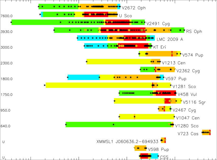
An updated description of the Swift archive of nova observations
was presented by Schwarz et al. (2011), focusing on comparisons of
the large monitoring programs. In the right panel of Fig. 1,
colour codes are used to mark different phases based on spectral
shapes and brightness, as described in the caption. The arrangement
in vertical direction is an indicator for the speed class, using the
full width at half maximum (FWHM) line width of optical lines (values
given in right and left).
With narrower FWHM (thus slower speed class), the SSS phase occurs
later in the evolution.
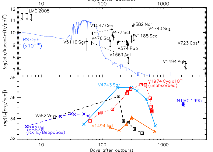
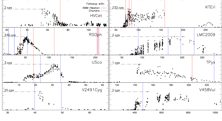
The long-term Swift X-ray (and partly simultaneous UV) light curves are presented, e.g., in Schwarz et al. (2011), eight of these are shown in Fig. 2, where XMM-Newton and Chandra observations are marked by blue and orange lines, respectively (see below). Each plot has a different y-scale, and to give an impression of the respective brightness levels, the maximum count rates are marked with a horizontal dashed line with values in units counts per second (cps) given in the left. Two orders of magnitude in count rate have been encountered.
The first dense Swift X-ray monitoring programme of a nova
was carried out following the 6th outburst of the recurrent
symbiotic nova RS Oph in February 2006 (Page et al. 2008; Osborne et al. 2011,
second panel in left column in Fig. 2).
The X-ray brightness evolution was followed until long after the
nova had turned off. The early shock phase, the SSS phase, and
the decline phases were all extremely well covered with brightness
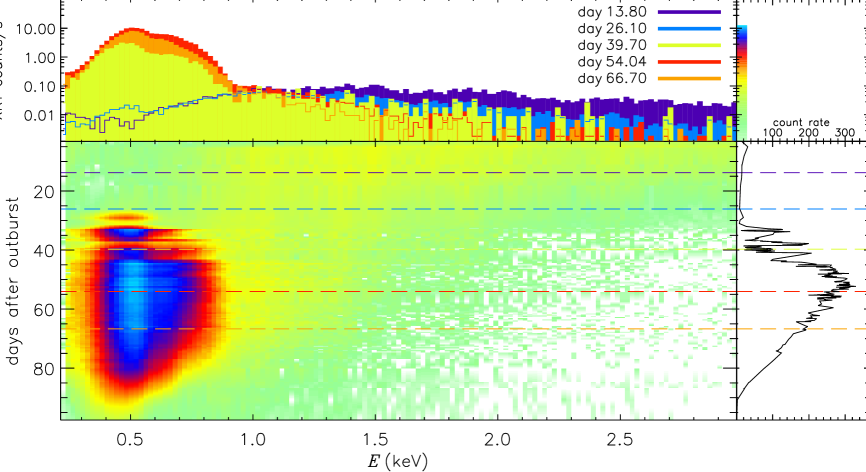
and spectral information. An illustration of the available Swift
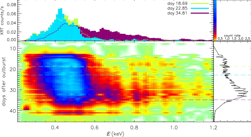
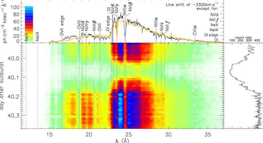
data is shown in the top plot in Fig. 3.
The early shock phase can be seen in the spectral brightness
map above 1 keV, while the later SSS phase covers the range
between 0.3-0.9 keV in energy and 30-90 days after outburst
in time. The early shock phase was analysed
by Bode et al. (2006), and the evolution of shock velocity was
derived, using the plasma temperature that was derived from
collisional plasma models to the Swift spectra. Later,
Vaytet et al. (2011) used hydrodynamic models yielding
much higher shock velocities, indicating that the gas
temperature from standard models is not the ideal way to
assess the shock velocity. In addition to high shock
velocities, a rather low ejecta mass was found. The models
were only applied to the low-resolution Swift spectra,
excluding the SSS component in the later observations.
While the standard models by Bode et al. (2006) also reproduce
the high-resolution grating spectra (Ness et al. 2009b), this
has not yet been tested with the hydro model used by Vaytet et al. (2011).
The evolution of RS Oph during the rise phase into the
SSS phase led to some initial confusion as the nova seemed
to turn off quicker than expected but then increased again
in flux (Osborne et al. 2006a). Continued monitoring revealed
a high-amplitude variability phase during the early SSS phase
(Osborne et al. 2006c). RS Oph turned out not to be unique in having an early
variability phase as other nova monitoring observations displayed the
same. For example, in the slower nova V458 Vul (Ness et al. 2009a), a
steep drop in count rate after the initial rise of SSS emission occurred
around day 410 (bottom right of Fig. 2). The on- and off states
during the early SSS phase were in fact strictly anticorrelated to the UV
(Schwarz et al. 2011). The same phenomenon was seen in several other novae
(see Fig. 2 and Schwarz et al. 2011), allowing the conclusion
that high-amplitude variations are a common phenomenon during
the early SSS phase of novae.
Light curve modelling of the Swift light curve of RS Oph was performed by Hachisu et al. (2007), who assume that the optically thick wind has stopped with the start of the SSS phase. The high-amplitude variations are neglected in the light curve model.
During the SSS phase of RS Oph, periodic variations of
seconds were present in the Swift and XMM-Newton X-ray light
curves (Osborne et al. 2006c, b; Ness et al. 2007b). The same 35-s period was
also found in Swift observations of KT Eri, leading Beardmore et al. (2010)
to conclude that it is not related to rotation but rather intrinsic,
e.g., nuclear burning instabilities. The complete set of
Swift X-ray spectra taken during the SSS phase of RS Oph were
studied in detail by Osborne et al. (2011). The low-resolution Swift
spectra were modeled with the same
atmosphere code in which a set of fixed parameters was chosen
in addition to which the evolution of effective temperature, line-of-sight
absorption (), radius, and luminosity was studied.
As in the case of the hydro model used by Vaytet et al. (2011), a
highly complex model fitted to low-resolution spectra needs to be
constrained by high-quality grating spectra, if available,
however, currently no atmosphere model has so far been
found that reproduces the grating spectra in all details. For
example, Nelson et al. (2008) present a preliminary model using the
same code used by Osborne et al. (2011), and it does not reproduce
the grating data. The assumed fundamental physics may thus be
wrong, but the approach is to consider only relative changes, and
Osborne et al. (2011) found that the early variability
phase was not only variable in brightness but also in
temperature and absorption.
A similar approach to find the underlying physical changes
that lead to spectral changes during the SSS phase were
presented by Page et al. (2010) using the monitoring data of
the fast nova V2491 Cyg (see bottom left panel of Fig. 2).
Instead of an atmosphere model,
a simple blackbody fit was used, yielding the same parameters,
effective temperature, , radius, and luminosity,
again only inspecting the relative changes, even though the
underlying physics of the model are not fully correct.
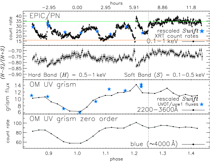
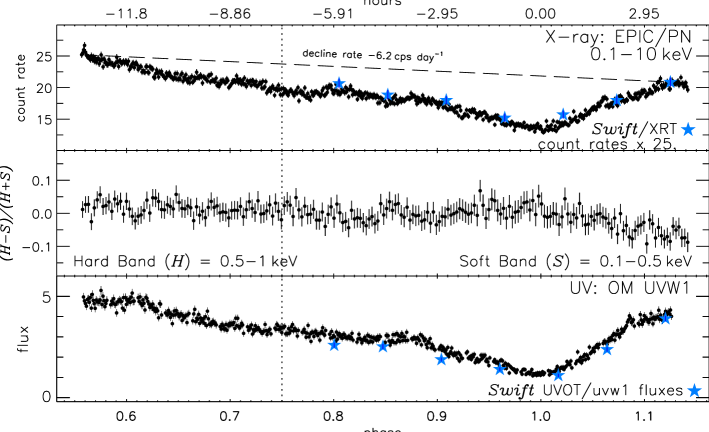
The recurrent nova U Sco had been overdue to explode again in 2009 (Schaefer 2005) and was monitored in optical very closely until the outburst was finally discovered in January 2010 (Schaefer et al. 2010). It’s particular importance arises from the fact that the binary system is seen edge on, yielding total eclipses (e.g., Schaefer 1990). Swift monitoring started immediately after outburst, with the first observation only 1.2 days after outburst. No detection in X-rays was found until the onset of the SSS phase (Schlegel et al. 2010). Consecutive Swift observations were centred around predicted eclipse times, but with a series of short snapshots, eclipses in X-rays were at most suggestive from phase-folded count rates (Osborne et al. 2010) from several cycles. A continuous XMM-Newton observation indicated X-ray dips rather than an eclipse (see Fig. 9 in Sect. 4.3). After day 30, the Swift count rates showed much clearer eclipses, and a second XMM-Newton observation was scheduled which then also contained a clear X-ray eclipse. The entire Swift light curve is shown in the third panel of the left column in Fig. 2 and the spectral evolution in the bottom panel of Fig. 3. Clearly recognized can be a conintuous increase in temperature with time.
4.2 Pre-Swift XMM-Newton/Chandra observations
The very first X-ray grating spectrum of a nova was
taken 2000, February 14 of V382 Vel which was found
in the SSS state in a Chandra ACIS observation of 1999,
December 30 (Burwitz, Starrfield, Krautter,
& Ness 2002). The resulting spectrum was
much fainter than expected, indicating that the nova had
turned off within only 2.5 months. The grating
spectrum was still useful as it displayed post-outburst
nebular emission lines that had never been seen before.
Ness, Starrfield, Jordan,
Krautter, & Schmitt (2005) inspected and analysed the data
using an emission measure distribution model. The line
profiles revealed double peaks indicative of different
kinematic components of the nebular plasma. Weak
continuum was seen that could arise from a
-K WD, indicating that
it had not yet cooled down after the
outburst. Under the assumption of collisional
equilibrium in a low-density plasma as in stellar
coronae, the distribution of kinetic (electron)
temperature could be reconstructed from line
ratios. From the inferred temperature distribution and
systematic deviations of predicted and measured
lines fluxes, the elemental abundances could be
derived. Although the nova had gone through an
earlier so-called Fe-curtain phase in the UV
(Shore et al. 2003), the X-ray spectrum contains
no Fe lines. The abundance diagnostics confirmed
that Fe was at least 4% underabundant with
respect to oxygen. Ness et al. (2005) argue that
instead of underabundant Fe, the elements that
produce the observed emission lines are overabundant.
Two more
Chandra observations of V382 Vel were taken with
the ACIS, without a
grating, and fading emission lines were visible,
also with the lower CCD resolution (Burwitz et al. 2002).
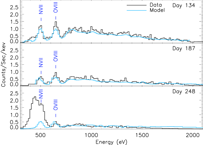

A few months later, the nova V1494 Aql offered another opportunity
to study nova evolution with Chandra. Without any knowledge
how bright the nova may be in X-rays, a blind shot was taken
with the ACIS on day 134 after outburst, and the 5-ks
observation yielded a hard spectrum with two resolved emission
lines but no signs of SSS emission (see Fig. 4).
Fortunately, significant X-ray emission was present already
before the SSS phase started, so more observations in
months intervals yielded secure results with good perspectives
for eventually finding SSS emission. On day 248, clear indications
for SSS emission arose, albeit still not quite as bright as
in other novae. On day 300, the grating was then employed,
yielding the first SSS spectrum of a nova in high resolution.
This spectrum is different than expected, showing continuum
plus emission lines. 4 days later, a deeper exposure was
taken, yielding a similar spectrum, thus the SSS spectrum
is not an atmospheric spectrum as expected. It may be related
to the high system inclination angle (Barsukova & Goranskii 2003)
(Ness et al. in preparation, and Fig. 11).
To this date,
no satisfactory spectral model could be found. For discussion
also on timing analysis, I refer to Rohrbach, Ness, &
Starrfield (2009). Without
any information how long the SSS phase may last, the next
observation was taken one year later, but the nova had already
turned off, yielding a weak detection only in the zero-th
order of the grating observation. 5 years later, Swift observed
again with no further detections (Sect. 4.1).
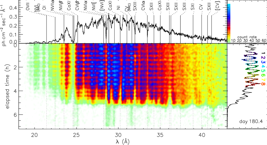
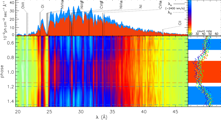
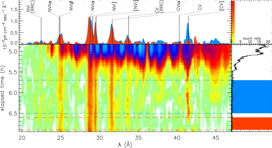
Also the nova V4743 Sgr (2002) had to be studied without additional information from other X-ray observatories. Again, in order to avoid non-detections in a long grating observation, a first, short, 5-ks, snapshot was taken in November 2002, two months after outburst. Again, a clear detection was found but no SSS spectrum. The nova was then not visible for 4 months, but as soon as it came back from behind the sun, a grating spectrum was taken (180.4 days after outburst), yielding the first really bright SSS spectrum with continuum and deep absorption lines from highly ionised species (Ness et al. 2003). A graphical illustration of the spectral evolution during this observation is shown in Fig. 5.
The observation starts with high-amplitude periodic variations, and eight clean cycles are marked with different colours in the light curve, turned around by 90o, in the right panel of Fig. 5. These eight cycles have been used to create a phase-folded light curve and corresponding spectral map, shown in the middle plot. The two spectra in the top are integrated over all phase minima and phase maxima, respectively, showing that the minima spectra are systematically softer. These periodic X-ray variations have been seen in all X-ray observations, including those taken post outburst. Detailed timing analyses have been carried out by Leibowitz et al. (2006); Dobrotka & Ness (2010), discovering the double nature of the frequency during the SSS phase which later merges into a single frequency (Dobrotka & Ness 2010).
About 2 hours before the end of the observation, the count rate suddenly dropped from 40-60 counts per second to nearly zero within very short time. No technical fault was identified, but a physical cause for such a steep decline was not easily found. At that time, the high-amplitude variations during the early SSS phase described above in Sect. 4.1 had not yet been discovered, and it appears plausible that this decline was in fact the first time this phenomenon was seen.
In the top plot, one can see that the harder part of the spectrum, shortward of Å, started earlier with the decline than the softer part, and that emission lines were left behind, both reported by Ness et al. (2003). The evolution of the faint emission lines after the decline is illustrated in the bottom, and one can see that some emission lines are variable. The forbidden line of C v (1sS0–1s2p 3S1) at 41.47 Å is much stronger than the 1sS0–1s2p 1P1 resonance line at 40.27 Å. While at about 5.7 hours after the start of the observation, the C v line disappears, it reappears between 6.0 and 6.6 hours, at first red shifted and then gradually changing to being blue shifted. If the C v emitting material originated from plasma that co-rotates with the WD at 2400 sec spin period, red/blue shifts of Å implied an orbital radius of 3 R⊙. It bears closer investigation, however, why a plasma so far away would not produce any resonance line emission.
The sudden decline triggered an XMM-Newton observation only two
weeks later (day 196.1 after outburst), in which the source was
as bright as before the decline started (Orio et al. 2003),
indicating that it was a transient phenomenon, strengthening
the link to the early high-amplitude variability phase (see
Sect. 4.1). Denser monitoring than
for V1494 Aql was chosen with three more observations on days
301.9, 371, and 526.1 after outburst, and all yield the same
general spectrum with some changes in temperature and
in several details, but no further decline as on day 180.6 was
seen.
All five SSS spectra of V4743 Sgr were modeled by Rauch et al. (2010)
using the Tübingen Model Atmosphere Package (TMAP), a non-LTE
atmosphere model that is optimised for hot
WDs. The evolution of the effective temperature was
described to have been reached on day 196.1, after which it
remained stable at least until day 371. A massive WD
of 1.1-1.2 M⊙ was deduced, and the photosphere was
found to be nitrogen-rich and carbon-deficient, indicative
of CNO cycle processed material. Under the assumption that
the observed photospheric emission arises from the surface of
the WD, it was concluded that some of the accreted material
was not ejected and remained instead on the WD.
Towards later observations, a reduced nitrogen abundance was
derived, implying that new, N-poorer material, was present
that may come from the companion via renewed accretion.
These conclusions may depend to some degree on the assumptions that, in spite of the complexity of the TMAP code, must still be considered somewhat simplified. Ness et al. (2011) argued that assumptions such as hydrostatic equilibrium and a plane parallel geometry are only valid in isolated hot WDs, for which the TMAP code is designed, but not in expanding nova ejecta. The blue shifts of the atmospheric absorption lines in the X-ray grating spectra give direct whitness of the continued expansion and thus a non-static environment. In the TMAP model, Rauch et al. (2010) introduced an artificial blue shift to better reproduce the data, but the entire atmosphere structure may be fundamentally different in an expanding environment. Attempts to model also the expansion in non-LTE radiative transport calculations have been made in the PHOENIX code (see, e.g., Hauschildt et al. 1992; Hauschildt & Baron 1999). Clearly, the complexity increases even further, but the X-ray grating spectra are of sufficient quality to use such approaches. The PHOENIX code was originally designed to model UV spectra, but has later been expanded to the X-ray regime (Petz et al. 2005) and improved by van Rossum (2009) with first results shown by van Rossum & Ness (2010) who found that atmosphere models that account for the expansion yield vastly different results from static models. Most recently, van Rossum (2012) presented a full description of a new model, based on PHOENIX, called "Wind-Type" (WT) SSS Nova Model, that will be made publicly available. The same five grating spectra of V4743 Sgr have been modeled, yielding different principal parameters than those found by Rauch et al. (2010). The effective temperatures are generally lower while is higher. The values found by van Rossum (2012) are in better agreement with Galactic neutral hydrogen maps of Kalberla et al. (2005) and Dickey & Lockman (1990) as implemented in the HEASARC Galactic tool111http://heasarc.nasa.gov/cgi-bin/Tools/w3nh/w3nh.pl yielding and cm-2, respectively. The differences between van Rossum (2012) and Rauch et al. (2010) can partly be explained by a different approach in determining , but the main difference is caused by two additional parameters, and in van Rossum (2012), parameterising the expansion. More work will be needed to investigate the effects of non-solar abundances. Well constrained model parameters will guide theoretical nova evolution models. The low-resolution spectra taken during Swift monitoring can be used to interpolate the models that have been constrained in detail by 2-3 grating spectra.
4.3 Swift-assisted XMM-Newton/Chandra observations
The greatest difficulty in getting grating spectra during
the SSS phase is finding the right moment. This has been
overcome with the use of Swift to get short snapshots
over much shorter time intervals (see Sect. 4.1).
The Swift count rates were used to calculate the
required grating exposure times.
The first time that the potentials of Swift for nova
studies were systematically explored was during the 2006
outburst of the recurrent, symbiotic, nova RS Oph.
Initial Swift observations established an extremely high
X-ray brightness level, with severe pile up in the
photon counting mode. There was no doubt that short
grating observations would be highly informative, and
simultaneous XMM-Newton and Chandra observations were
organised to take place only two weeks after outburst.
While Swift monitoring continued, grating observations
were taken whenever significant changes in brightness
and spectral shape were seen with Swift, yielding a
total of three XMM-Newton and three Chandra observations
before the end of the SSS phase (see 2nd panel in
left row of Fig. 2). The
nova remained interesting also after it turned off,
and more grating observations were taken. An overview
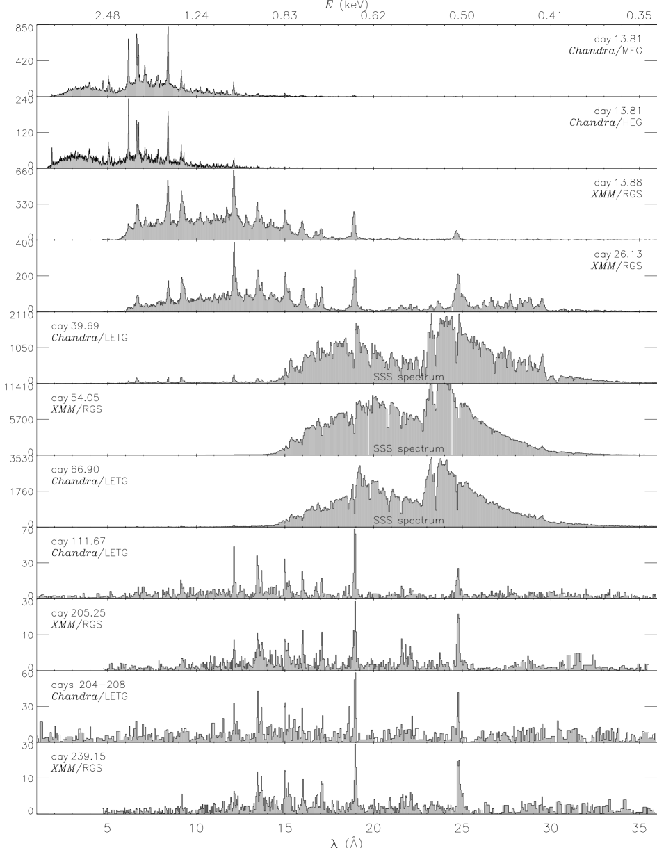
of the grating observations was given by Ness et al. (2009b)
which is reproduced in Fig. 8. The first two
spectra were extracted from the two grating arms of the
Chandra/HETGS, the Medium Energy Grating (MEG) and the
High Energy Grating (HEG). These observations were
taken simultaneously with the XMM/RGS (third
spectrum in Fig. 8).
The top four spectra in Fig. 8 were taken
during the shock phase,
before the SSS phase started while, in the symbiotic
system, the nova ejecta ran through the dense
stellar wind of the giant companion star, dissipating
significant amounts of kinetic energy during shocks
that was partially converted to X-ray emission.
The X-ray spectrum is that of a plasma in collisional
equilibrium, evidenced by line ratios of He-like
emission lines of Mg (Nelson et al. 2008). Two different groups
have analysed the same spectra in different ways:
Nelson et al. (2008) applied an xspec (Arnaud 1996)
multi-temperature model with solar abundances,
needing 4 temperature components.
Ness et al. (2009b) used two approaches, first
the same as Nelson et al. (2008) but with variable
abundances, needing then only three temperature
components. High overabundance of Mg and Si
and underabundance of Fe, relative to oxygen, were found.
Since a plasma
of three distinct temperature components is not
necessarily physically realistic, Ness et al. (2009b)
also applied the same method already used for
V382 Vel assuming a continuous temperature
distribution (see above and Ness et al. 2005) and
found the same general abundance trends but with
better constraints of N and S. Comparison of the
abundances with those in single giants revealed
considerable anomalies suggesting that the companion
in RS Oph has changed substantially by the
continued mass loss via accretion. Alternatively,
these abundances would reflect the composition of the
WD which would question the system
to be a SN Ia progenitor which requires a
carbon-oxygen rich (CO) WD while
the observed abundances in the X-ray plasma
would indicate more an oxygen-neon (ONe) white
dwarf. The difference in nuclear binding energy
between elements (such as neon, magnesium,
silicon) and iron is not sufficient to disrupt
the WD while nuclear fusion chain reactions
starting from carbon, as found in a CO WD, produce
more energy.
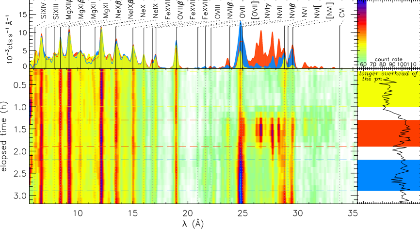
The SSS phase of RS Oph may have started during
the XMM-Newton observation taken on day 26.1 in
which Nelson et al. (2008) observed the appearance of a new
soft component. While the high-energy part of the spectrum
(fourth panel in Fig. 8) could be
modelled with the same approaches of collisional
plasma as for day 13.8 (Ness et al. 2009b), the new
soft component between Å coincides
in wavelength with the soft tail of the later SSS
phase (see fourth and fifth panels in
Fig. 8). In a low-resolution spectrum,
the new component would have been interpreted as first
signs of atmospheric emission, and a blackbody fit
to the simultaneous XMM-Newton/MOS spectrum yields
indeed a good fit. However, in the high-resolution RGS
spectrum, several unknown overlapping emission lines
can be seen, quite atypical of SSS emission. An
illustration of the time evolution of the appearance
of the new soft component during the observation is
given with Fig. 6. Only two
lines of N vi (1s-2p triplet) at 28.8-29.5 Å and N vii (1s-2p doublet) plus N vi (1s-3p)
at Å can be identified while all other
features are of unknown origin. Nelson et al. (2008)
speculate these may be highly blue-shifted 1s-3p and
1s-4p lines of C vi, but the principle
C vi 1s-2p line at 33.8 Å is not present
(see Fig. 6), and also the C
abundance was argued in other context of the same
article to be extremely low. From Fig. 6
it can be seen that the unknown emission features
were present for only 40-50 minutes (between the
two horizontal dashed red lines), suggesting these
may be instable transitions, e.g., between excited states.
A conclusive interpretation of the day-26.1 spectrum
of RS Oph is still outstanding but important as it may hold
clues of the transition into the SSS phase.
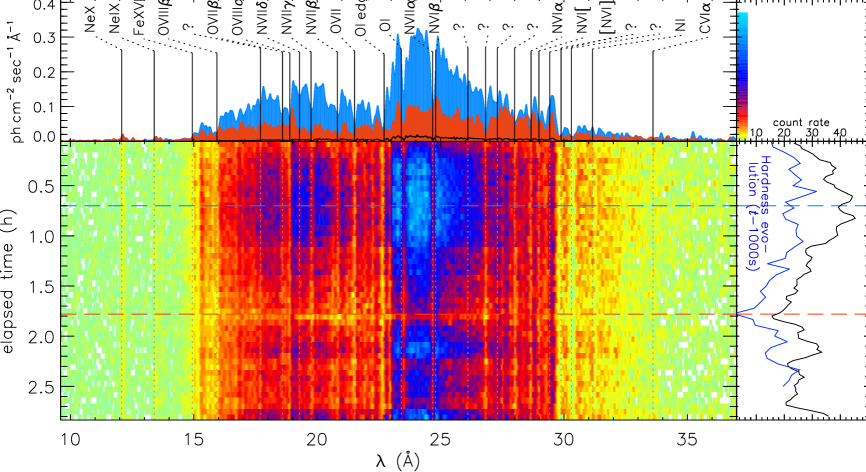
A few days later, Swift observed a steep rise into the SSS phase, and a Chandra LETG observation was scheduled which fell, however, into an unanticipated low state that occurred soon after. Nevertheless, an extremely well exposed spectrum was obtained. Continued Swift monitoring allowed scheduling of two more grating observations during the peak and decline of the SSS phase (see Fig. 2). The time evolution of this observation is illustrated in Fig. 7. Also on shorter time scales, the nova was highly variable. A 1000-s delay between brightness and hardness light curves in the day 39.7 (see right panel of Fig. 7) observation led Ness et al. (2007b) to conclude that photoionisation of neutral oxygen led to variations in transparency, allowing more (harder) X-ray light to escape when oxygen is ionised. Considerable reductions in the depth of the neutral oxygen edge towards the later observations support this conclusion.
Based on the Swift light curve of the famous recurrent nova
U Sco, shown in the third panel of the left column in
Fig. 2 and the bottom plot in Fig. 3,
an initial Chandra observation was scheduled on day 18.7 after
outburst but was not centred around eclipse. Later,
on day 22.9, a longer continuous XMM-Newton observation
was scheduled that resolved the details of the
X-ray brightness during optical eclipses.
Guided by the contemporaneous OM light curve that
clearly showed an eclipse, Ness et al. (2012) showed that dips
occurred between quadratures (phases -0.75 to 0.25; see
left panel in Fig. 9).
A few days later, the Swift count rates showed clear
eclipses, and a second XMM-Newton observation was
scheduled to resolve the details (see right panel in
Fig. 9). The X-ray spectrum
during the SSS phase was atypical again, with strong
emission lines on top of blackbody-like continuum,
resembling the proto typical SSS Cal 87 in the LMC,
which is also an eclipsing system. Ebisawa et al. (2010)
discussed the possibility that the accretion disk in
Cal 87 blocks the central emission from the WD,
and all observable X-ray emission originates from
Thomson scattering within the Accretion Disk Corona
(ADC). Additional resonance line scattering can produce
the observed emission lines. To transfer these
conclusions to U Sco, an accretion disk must already
have been present or in the process of re-establishment.
The dips in X-rays can be explained by neutral clumpy
material within an accretion stream from the companion
star. Neutral gas is transparent to UV/optical light
but opaque to X-rays. Once the accretion disk has flattened,
no more dips are seen in X-rays.
The very fast nova V2491 Cyg entered the SSS phase just
a bit more than a month after outburst. Guided by the Swift
snapshots (see bottom left panel in Fig. 2), two
XMM-Newton observations were triggered in short succession,
on days 39.9 and 49.6, both extremely well exposed. Without
Swift, this quick evolution could not have been followed.
Significant X-ray variability was found on day 39.9
(Ness et al. 2011, see Fig. 10).
The absorption lines were highly blue shifted indicating
high expansion velocities. Ness et al. (2011) also showed
that currently publicly available atmosphere models are
not sufficient to reproduce these high-quality spectra.
Preliminary PHOENIX atmosphere models to the V2491 Cyg
spectra were presented by van Rossum & Ness (2010), using
a combination of a hydrostatic core and a hydrodynamic
expanding envelope. The additional expanding envelope
yields a clearly better fit to the data, but the large
majority of absorption lines are not reproduced.
Pinto et al. (2012) developed a new approach using a multicomponent
SPEX (Kaastra et al. 1996) model, consisting of emission and absorption
components, but also this approach did not reproduce the
spectra in a formally satisfactory way.
The classical nova KT Eri was followed with four Chandra
observations. The nova was extremely bright (Bode et al. 2010)
that extremely short exposures of only a few seconds
were needed to already obtain extremely well exposed spectra
(Ness et al. 2010). Again, these grating spectra are extremely
complex.
5 Conclusions
While results from individual observations have already been discussed in the previous sections, I focus here on more general conclusions that can be drawn from the entirety of all observations.
5.1 Pre- and Post-SSS phase
Originally, novae were only expected to be X-ray sources
during their SSS phase, when the photospheric radius had
receded into the nuclear burning regions near the surface
of the WD. However, already the earliest X-ray observations
of novae have revealed pre-SSS X-ray emission, e.g., in
V838 Her (O’Brien et al. 1994) or V1974 Cyg (Krautter et al. 1996).
Plasma models to the low-resolution data indicate that
the emission arises from a collisional plasma and
is suspected to originate in shock fronts within the ejecta
(e.g., Brecher et al. 1977). An “interacting
winds” model has been developed by
O’Brien et al. (1994) and was refined by Lloyd et al. (1995)
for the specific case of V838 Her. They argued
that the shock-heating must take place as a result
of the interaction of different components
within the ejecta.
The much increased sample of X-ray observed novae with
the new-generation X-ray observatories gives an idea
of the frequency of early hard emissions. Out of
27 novae that have been observed with Swift within
the first 100 days after outburst with at least two
observations, 11 were detected but without an SSS component
in the first observation and 17 in the second observation.
Thus about half of all novae display pre-SSS X-ray emission.
The interacting winds model predicts inhomogeneities
within the ejecta, and these may have left their footprints
also in the later SSS grating spectra that contain complex
absorption line profiles indicating different velocity
components (see, e.g., Ness et al. 2011).
It needs to be kept in mind that the early spectra of
RS Oph have a different origin with shocks between
the ejecta and the stellar wind of the companion that is
less dense in main sequence companions. This produces much
more X-ray emission than intra-ejecta shocks.
Owing to their intrinsic faintess, intra-ejecta shock
spectra have never been observed with an X-ray grating.
Post-SSS grating spectra were taken of V382 Vel and of RS Oph, both yielding faint emission line spectra. While V382 Vel contains multiple velocity components, the spectral lines in RS Oph are single. Both spectra can be modeled by collisional plasma models, which is not necessarily trivial with grating spectra. The post-SSS emission phase likely originates in radiatively cooling nebular ejecta (e.g., Ness et al. 2005) which can be highly non-solar in composition.
5.2 SSS phase
The new observations during the SSS phase have
revealed a number of unexpected complications
such as high-amplitude variations during the early
SSS phase (see Sect. 4.1),
extremely complex high-resolution spectra,
and a high degree of diversity.
The expected form of an SSS spectrum was an atmospheric absorption line spectrum. However, the first ever nova that was observed during the SSS phase with a grating, V1494 Aql, displayed a completely different spectrum (see right panel of Fig. 4), and spectral modelling was so far unsuccessful (Rohrbach et al. 2009). The second observed nova SSS spectrum, of V4743 Sgr, complied better with expectations (see Fig. 5), but the light curve was violently variable with the mysterious decline that only years later can be seen in the context of the early variability phase. The high degree of diversity was unexpected, and only with more observations, some similarities were found, for example a remarkable similarity between the SSS spectra of RS Oph and V2491 Cyg (Ness et al. 2011). Spectral modelling of SSS spectra still leaves too many doubts to lead to conclusive results. Not a single approach has so far led to satisfactory reproduction of the observed spectra in a statistical sense. Attempts were made with:
-
1.
The non-LTE WD atmosphere model TMAP (Rauch et al. 2010)
-
2.
The expanding radiative transfer model based on PHOENIX (van Rossum 2012)
-
3.
A multicomponent SPEX model (Pinto et al. 2012).
TMAP is currently the best tested approach and is available to the
scientific community, however, the expansion of the absorbing plasma,
proven by the observed line blue shifts, invalidates the assumptions
of hydrostatic equilibrium and plane parallel geometry. An approach to
compute radiative transport in a co-moving frame has been
implemented in the PHOENIX code, and van Rossum & Ness (2010)
have shown that hydrostatic and hydrodynamic models lead
to different spectra, and adjustments to observed spectra
lead to different key parameters. The conclusions drawn from
TMAP modelling are therefore to be treated with care. The PHOENIX
code may be more promising as demonstrated by van Rossum (2012).
Although currently only models with solar abundances are available,
already good agreement between models and data has been found.
These models will be publicly available and could be used to
parameterise individual grating spectra and then using these
models to interpolate along the low-resolution Swift spectra
to get the full evolution of the atmosphere parameters at the
time density of the Swift monitoring. The approach by
Pinto et al. (2012) of combining emission- and absorption components
in a self-consistent way may be a promising alternative, but one
has to be careful to use the large number of degrees of freedom
wisely.
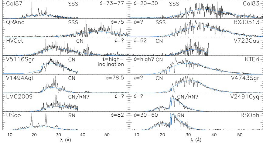
The studies of U Sco have given more clues, as the eclipsing system displayed an SSS spectrum that resembles the also eclipsing proto-typical SSS Cal 87 (Ebisawa et al. 2010). There is reason to believe that high-inclination systems contain stronger emission line components with less-pronounced absorption lines than low-inclination systems. In Fig. 11, 14 grating SSS spectra are shown in comparison. The light blue lines guide the eye that all sources contain photospheric continuum emission that has the shape of a blackbody. More detailed discussion will be presented in an upcoming paper Ness et al. in preparation. An inclination-angle dependence indicates asymmetric ejecta and possibly the presence of renewed accretion. If we are dealing with clumpy accretion, the early variability phase could be explained as temporary ocultations of the central source that cease when a flatter accretion disk has formed.
References
- Arnaud (1996) Arnaud K. A., 1996, in Astronomical Society of the Pacific Conference Series, Vol. 101, Astronomical Data Analysis Software and Systems V, Jacoby G. H., Barnes J., eds., p. 17
- Balman et al. (1998) Balman S., Krautter J., Ögelman H., 1998, ApJ, 499, 395
- Barsukova & Goranskii (2003) Barsukova E. A., Goranskii V. P., 2003, Astronomy Letters, 29, 195
- Beardmore et al. (2010) Beardmore A. P. et al., 2010, The Astronomer’s Telegram, 2423, 1
- Bode & Evans (2008) Bode M. F., Evans A., 2008, Classical Novae, Bode, M. F. & Evans, A., ed. Cambridge University Press
- Bode et al. (2006) Bode M. F. et al., 2006, ApJ, 652, 629
- Bode et al. (2010) Bode M. F. et al., 2010, The Astronomer’s Telegram, 2392, 1
- Brecher et al. (1977) Brecher K., Ingham W. H., Morrison P., 1977, ApJ, 213, 492
- Burrows et al. (2005) Burrows D. N. et al., 2005, Space Science Reviews, 120, 165
- Burwitz et al. (2002) Burwitz V., Starrfield S., Krautter J., Ness J.-U., 2002, in AIP Conf. Proc.: Classical Nova Explosions, Hernanz M., José J., eds., Vol. 637, American Institute of Physics, p. 377
- den Herder et al. (2001) den Herder J. W. et al., 2001, A&A, 365, L7
- Dickey & Lockman (1990) Dickey J. M., Lockman F. J., 1990, ARAA, 28, 215
- Dobrotka & Ness (2010) Dobrotka A., Ness J., 2010, MNRAS, 405, 2668
- Ebisawa et al. (2010) Ebisawa K., Rauch T., Takei D., 2010, AN, 331, 152
- Gallagher & Starrfield (1976) Gallagher J. S., Starrfield S., 1976, MNRAS, 176, 53
- Greiner et al. (1991) Greiner J., Hasinger G., Kahabka P., 1991, A&A, 246, L17
- Hachisu et al. (2007) Hachisu I., Kato M., Luna G. J. M., 2007, ApJ, 659, L153
- Hartmann & Heise (1997) Hartmann H. W., Heise J., 1997, A&A, 322, 591
- Hauschildt & Baron (1999) Hauschildt P. H., Baron E., 1999, Journal of Computational and Applied Mathematics, 109, 41
- Hauschildt et al. (1992) Hauschildt P. H., Wehrse R., Starrfield S., Shaviv G., 1992, ApJ, 393, 307
- Kaastra et al. (1996) Kaastra J. S., Mewe R., Nieuwenhuijzen H., 1996, in UV and X-ray Spectroscopy of Astrophysical and Laboratory Plasmas, K. Yamashita & T. Watanabe, ed., p. 411
- Kahabka et al. (1994) Kahabka P., Pietsch W., Hasinger G., 1994, A&A, 288, 538
- Kahabka & van den Heuvel (1997) Kahabka P., van den Heuvel E. P. J., 1997, ARA&A, 35, 69
- Kalberla et al. (2005) Kalberla P. M. W., Burton W. B., Hartmann D., Arnal E. M., Bajaja E., Morras R., Pöppel W. G. L., 2005, A&A, 440, 775
- Krautter (2002) Krautter J., 2002, in American Institute of Physics Conference Series, Vol. 637, Classical Nova Explosions, M. Hernanz & J. José, ed., p. 345
- Krautter (2008) Krautter J., 2008, in Astronomical Society of the Pacific Conference Series, Vol. 401, RS Ophiuchi (2006) and the Recurrent Nova Phenomenon, A. Evans, M. F. Bode, T. J. O’Brien, & M. J. Darnley, ed., p. 139
- Krautter et al. (1996) Krautter J., Ögelman H., Starrfield S., Wichmann R., Pfeffermann E., 1996, ApJ, 456, 788
- Leibowitz et al. (2006) Leibowitz E., Orio M., Gonzalez-Riestra R., Lipkin Y., Ness J., Starrfield S., Still M., Tepedelenlioglu E., 2006, MNRAS, 371, 424
- Lloyd et al. (1995) Lloyd H. M., O’Brien T. J., Bode M. F., 1995, Ap&SS, 233, 317
- Long et al. (1981) Long K. S., Helfand D. J., Grabelsky D. A., 1981, ApJ, 248, 925
- Nelson et al. (2008) Nelson T., Orio M., Cassinelli J. P., Still M., Leibowitz E., Mucciarelli P., 2008, ApJ, 673, 1067
- Ness et al. (2009a) Ness J. et al., 2009a, AJ, 137, 4160
- Ness et al. (2010) Ness J., Drake J. J., Starrfield S., Bode M., Page K., Beardmore A., Osborne J. P., Schwarz G., 2010, The Astronomer’s Telegram, 2418, 1
- Ness et al. (2009b) Ness J. et al., 2009b, AJ, 137, 3414
- Ness et al. (2011) Ness J. et al., 2011, ApJ, 733, 70
- Ness et al. (2012) Ness J. et al., 2012, ApJ, 745, 43
- Ness et al. (2008) Ness J., Schwarz G., Starrfield S., Osborne J. P., Page K. L., Beardmore A. P., Wagner R. M., Woodward C. E., 2008, AJ, 135, 1328
- Ness et al. (2007a) Ness J., Schwarz G. J., Retter A., Starrfield S., Schmitt J. H. M. M., Gehrels N., Burrows D., Osborne J. P., 2007a, ApJ, 663, 505
- Ness et al. (2007b) Ness J. et al., 2007b, ApJ, 665, 1334
- Ness et al. (2003) Ness J. et al., 2003, ApJL, 594, L127
- Ness et al. (2005) Ness J., Starrfield S., Jordan C., Krautter J., Schmitt J. H. M. M., 2005, MNRAS, 364, 1015
- O’Brien et al. (1994) O’Brien T. J., Lloyd H. M., Bode M. F., 1994, MNRAS, 271, 155
- Oegelman et al. (1987) Oegelman H., Krautter J., Beuermann K., 1987, A&A, 177, 110
- Orio et al. (2003) Orio M. et al., 2003, IAUcirc, 8131, 2
- Osborne et al. (2006a) Osborne J. et al., 2006a, The Astronomer’s Telegram, 764, 1
- Osborne et al. (2006b) Osborne J. et al., 2006b, The Astronomer’s Telegram, 801, 1
- Osborne et al. (2006c) Osborne J. et al., 2006c, The Astronomer’s Telegram, 770, 1
- Osborne et al. (2011) Osborne J. P. et al., 2011, ApJ, 727, 124
- Osborne et al. (2010) Osborne J. P. et al., 2010, The Astronomer’s Telegram, 2442, 1
- Page et al. (2008) Page K. L., Osborne J. P., Beardmore A. P., Goad M. R., Wynn G. A., Bode M. F., O’Brien T. J., 2008, in Astronomical Society of the Pacific Conference Series, Vol. 401, Astronomical Society of the Pacific Conference Series, A. Evans, M. F. Bode, T. J. O’Brien, & M. J. Darnley, ed., p. 283
- Page et al. (2010) Page K. L. et al., 2010, MNRAS, 401, 121
- Petz et al. (2005) Petz A., Hauschildt P. H., Ness J.-U., Starrfield S., 2005, A&A, 431, 321
- Pinto et al. (2012) Pinto C., Ness J.-U., Verbunt F., Kaastra J. S., Costantini E., Detmers R. G., 2012, A&A, 543, A134
- Rauch et al. (2010) Rauch T., Orio M., Gonzales-Riestra R., Nelson T., Still M., Werner K., Wilms J., 2010, ApJ, 717, 363
- Rohrbach et al. (2009) Rohrbach J. G., Ness J., Starrfield S., 2009, AJ, 137, 4627
- Roming et al. (2005) Roming P. W. A. et al., 2005, Space Science Reviews, 120, 95
- Schaefer (1990) Schaefer B. E., 1990, ApJL, 355, L39
- Schaefer (2005) Schaefer B. E., 2005, ApJL, 621, L53
- Schaefer et al. (2010) Schaefer B. E. et al., 2010, AJ, 140, 925
- Schlegel et al. (2010) Schlegel E. M. et al., 2010, The Astronomer’s Telegram, 2419, 1
- Schwarz et al. (2011) Schwarz G. J. et al., 2011, ApJS, 197, 31
- Shore et al. (2003) Shore S. N. et al., 2003, AJ, 125, 1507
- Starrfield et al. (2008) Starrfield S., Iliadis C., Hix W. R., 2008, in Classical Novae, Bode M., Evans A., eds., Cambridge University Press, p. 77
- Strüder et al. (2001) Strüder L. et al., 2001, A&A, 365, L18
- Turner et al. (2001) Turner M. J. L. et al., 2001, A&A, 365, L27
- van Rossum (2009) van Rossum D., 2009, Ph.D. Thesis, University of Hamburg
- van Rossum & Ness (2010) van Rossum D., Ness J., 2010, AN, 331, 175
- van Rossum (2012) van Rossum D. R., 2012, ArXiv e-prints
- Vaytet et al. (2011) Vaytet N. M. H., O’Brien T. J., Page K. L., Bode M. F., Lloyd M., Beardmore A. P., 2011, ApJ, 740, 5