Optimality Properties, Distributed Strategies, and Measurement-Based Evaluation of Coordinated Multicell OFDMA Transmission

Abstract

The throughput of multicell systems is inherently limited by interference and the available communication resources. Coordinated resource allocation is the key to efficient performance, but the demand on backhaul signaling and computational resources grows rapidly with number of cells, terminals, and subcarriers. To handle this, we propose a novel multicell framework with dynamic cooperation clusters where each terminal is jointly served by a small set of base stations. Each base station coordinates interference to neighboring terminals only, thus limiting backhaul signalling and making the framework scalable. This framework can describe anything from interference channels to ideal joint multicell transmission.

The resource allocation (i.e., precoding and scheduling) is formulated as an optimization problem (P1) with performance described by arbitrary monotonic functions of the signal-to-interference-and-noise ratios (SINRs) and arbitrary linear power constraints. Although (P1) is non-convex and difficult to solve optimally, we are able to prove: 1) Optimality of single-stream beamforming; 2) Conditions for full power usage; and 3) A precoding parametrization based on a few parameters between zero and one. These optimality properties are used to propose low-complexity strategies: both a centralized scheme and a distributed version that only requires local channel knowledge and processing. We evaluate the performance on measured multicell channels and observe that the proposed strategies achieve close-to-optimal performance among centralized and distributed solutions, respectively. In addition, we show that multicell interference coordination can give substantial improvements in sum performance, but that joint transmission is very sensitive to synchronization errors and that some terminals can experience performance degradations.

I Introduction

In conventional cellular systems, each terminal belongs to one cell at a time and data transmission is scheduled autonomously by its base station. We consider systems where each base station can divide its transmit resources between terminals using orthogonal frequency-division multiple access (OFDMA), which generates independent subcarriers [1]. In addition, multiple terminals can be assigned to each subcarrier using space division multiple access (SDMA) and multiple-input multiple-output (MIMO) techniques that manage co-terminal interference within the cell [2]. However, with base stations performing autonomous single-cell processing, the performance is fundamentally limited by interference from other cells—especially for terminals close to cell edges.

The limiting inter-cell interference can be handled by base station coordination, recently termed network MIMO [3] and coordinated multi-point transmission (CoMP) [4]. By sharing data and channel state information (CSI) over the backhaul, base stations can coordinate the interference caused to adjacent cells, and cell edge terminals can be jointly served through multiple base stations [5, 6, 7]. The multicell capacity was derived in [8], while more practical performance gains over conventional single-cell processing were reported in [9, 10, 11] under constrained backhaul signaling. In practice, the transmission optimization is also constrained by computational complexity and the difficulty of obtaining reliable CSI, which makes centralized implementations of multicell coordination intractable in large networks [11].

In practical multicell systems, only a small subset of base stations will take the interference generated at a given terminal into consideration (to limit the backhaul signaling and complexity, and to avoid estimating negligibly weak channels). Fixed cooperation clusters were considered in [9] to (iteratively) coordinate transmissions within each cluster. While easily implementable for co-located base stations (such as sectors connected to the same eNodeB in an LTE system), the performance is still limited by out-of-cluster interference. A more dynamic approach was taken in [12] where base stations serve partially overlapping sets of terminals. Still, global interference coordination was assumed, making the approach infeasible in large systems.

Resource allocation is very difficult to solve optimally, even under simplifying assumptions such as a single subcarrier, global interference coordination, and perfect CSI. A few type of problems can be solved using uplink-downlink duality [Boche2002a, Wiesel2006a, Yu2007a, Dahrouj2010a], but weighted sum rate optimization and similar problems are all NP-hard [Liu2011a]. There are algorithms that find the optimal solutions [Brehmer2010a, Bjornson2012a], but with unpractically slow convergence. Suboptimal iterative solutions that perform well on synthetic channels have been suggested in [Tolli2009b, Zheng2008a, 12, Venturino2010a]. However, synthetic and real channels usually differ due to the simplifications used in the channel model assumptions. The performance of downlink multicell coordination has not been evaluated on measured channels, thus characteristics such as the correlation between channels from different base stations have not been considered [Jalden2007a].

Herein, we analyze coordinated multicell OFDMA transmission, derive properties of the optimal resource allocation, propose low-complexity strategies, and analyze the performance on measured channels. The major contributions are:

• We propose a general multicell cooperation framework that enables unified analysis of anything from interference channels to ideal network MIMO. The main characteristic is that each base station is responsible for the interference caused to a set of terminals, while only serving a subset of them with data (to limit backhaul signaling).

• Multicell OFDMA transmission and resource allocation is formulated as an optimization problem (P1) with arbitrary monotonic utility functions (e.g., representing data rates, error rates, or mean square errors), single user detection, and arbitrary linear power constraints.

• Three properties of the optimal solution to (P1) are derived: 1) Optimality of single-stream beamforming; 2) Conditions for full power usage; 3) An explicit precoding parametrization based on a few real-valued parameters between zero and one. This novel parametrization improves prior work in [Jorswieck2008b, Bjornson2010c, Shang2010a, Zhang2010a, Mochaourab2011a] by supporting general multicell and multicarrier systems and generally requiring much fewer parameters.

• Two low-complexity strategies for resource allocation are proposed based on the three optimality properties and an efficient algorithm for subcarrier allocation. The centralized strategy provides close-to-optimal performance, while the distributed version is suitable for large systems with many subcarriers and where the backhaul and computational resources required for the iterative solutions in [Tolli2009b, Zheng2008a, 12, Venturino2010a] are unavailable.

• As the performance of any communication system depends on the channel characteristics, realistic conditions are necessary for reliable evaluation. Therefore, the proposed strategies are evaluated on measured channel vectors from a typical urban macro-cell environment. The impact of multicell coordination is evaluated both in terms of average performance and for fixed terminal locations, and the robustness to synchronization imperfections is studied.

Preliminary single-carrier results were reported in [Bjornson2010d].

Notation: $\mathbf{X}^{T}$, $\mathbf{X}^{H}$, and $\mathbf{X}^{\dagger}$ denote the transpose, the conjugate transpose, and the Moore-Penrose inverse of $\mathbf{X}$, respectively. $\mathbf{I}_{N}$ and $\mathbf{0}_{N}$ are $N\times N$ identity and zero matrices, respectively. If $\mathcal{S}$ is a set, then its members are $\mathcal{S}(1),\ldots,\mathcal{S}(|\mathcal{S}|)$ where $|\mathcal{S}|$ is the cardinality.

II General Multicell System Model

We consider a downlink system with $K_{t}$ transmitters, where transmitter $j$ is equipped with $N_{j}$ antennas. They communicate over $K_{c}$ independent subcarriers with $K_{r}$ receivers having one effective antenna each. The transmitters and receivers are denoted $\textrm{BS}_{j}$ and $\textrm{MS}_{k}$, respectively, for $j\in\mathcal{J}=\{1,\ldots,K_{t}\}$ and $k\in\mathcal{K}=\{1,\ldots,K_{r}\}$.

In a general multicell scenario, some terminals are served in a coordinated manner by multiple transmitters. In addition, some transmitters and receivers are very far apart, making it impractical to estimate and separate the interference on these channels from the noise. Based on these observations, we propose a general multicell coordination framework:

Definition 1.

Dynamic cooperation clusters means that $\textrm{BS}_{j}$

• Has channel estimates to receivers in $\mathcal{C}_{j}\subseteq\{1,\!...,\!K_{r}\!\}$, while interference generated to receivers $\bar{k}\not\in\mathcal{C}_{j}$ is negligible and can be treated as background noise;

• Serves the receivers in $\mathcal{D}_{j}\subseteq\mathcal{C}_{j}$ with data.

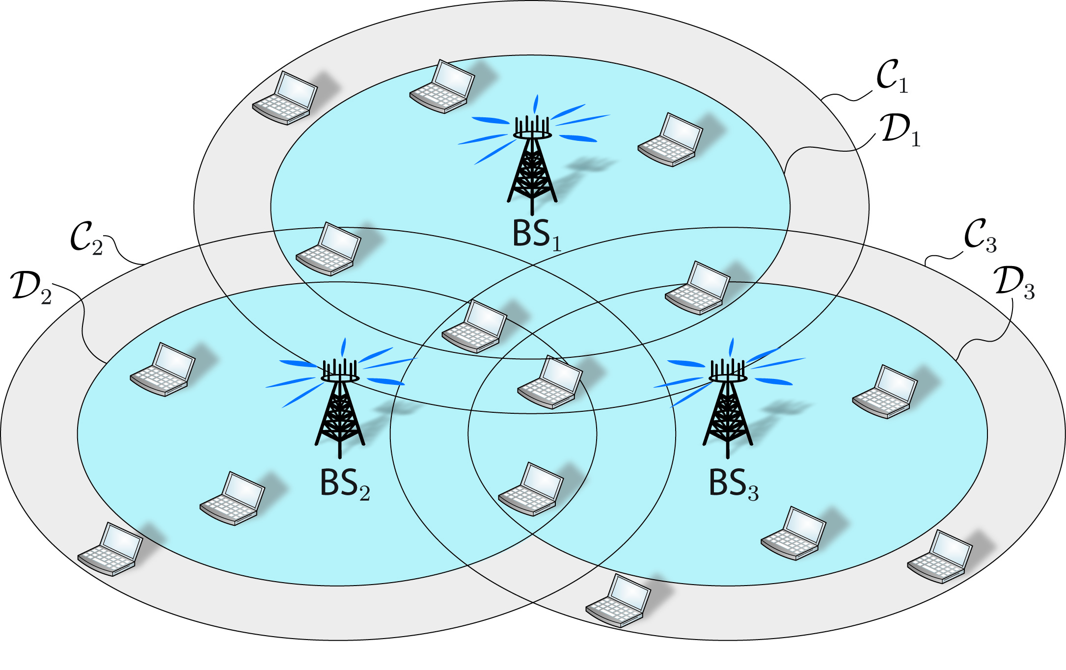
Figure 1: Intersection between three cells. $\textrm{BS}_{j}$ serves terminals in the inner circle ($\mathcal{D}_{j}$) and coordinates interference to terminals in the outer circle ($\mathcal{C}_{j}$). Ideally, negligible interference is caused to terminals outside both circles.

This coordination framework is characterized by the sets $\mathcal{C}_{j},\mathcal{D}_{j}$ for all $j\in\mathcal{J}$, which are illustrated in Fig. 1. The mnemonic rule is that $\mathcal{D}_{j}$ describes data from transmitter $j$, while $\mathcal{C}_{j}$ describes coordination from transmitter $j$. How to select these sets efficiently, by only accepting the overhead involved in interference coordination and joint transmission if the expected performance gains are substantial, is a very interesting and important problem. The solution depends on the system architecture and is beyond the scope of this paper (see [Zhang2004b, Fuchs2006a, 4, Xu2010a]), but a simple scheme would be to include $\textrm{MS}_{k}$ in $\mathcal{C}_{j}$ if the long-term average channel gain from $\textrm{BS}_{j}$ is above a certain threshold. If the gain is above a second threshold, the terminal is also included in $\mathcal{D}_{j}$. In principle, different $\mathcal{C}_{j},\mathcal{D}_{j}$ can be used for each subcarrier, but it is not necessary since subcarrier allocation naturally appears in the resource allocation analyzed herein. Observe that although $\mathcal{C}_{j},\mathcal{D}_{j}$ can be selected decentralized at transmitter $j$, some mechanism for coordination and data sharing is required between adjacent transmitters.

At subcarrier $c$, the channel from $\textrm{BS}_{j}$ to $\textrm{MS}_{k}$ is denoted $\mathbf{h}_{jkc}\in\mathbb{C}^{N_{j}\times 1}$. The collective channel from all transmitters is $\mathbf{h}_{kc}=[\mathbf{h}_{1kc}^{T}\ldots\mathbf{h}_{K_{t}kc}^{T}]^{T}\in\mathbb{C}^{N}$, where $N=\sum_{j\in\mathcal{J}}N_{j}$ is the total number of transmit antennas. Based on the framework in Definition 1, only certain channel elements in $\mathbf{h}_{kc}$ will carry data and/or non-negligible interference. These can be selected by the diagonal matrices $\mathbf{D}_{k}\in\mathbb{C}^{N\times N}$ and $\mathbf{C}_{k}\in\mathbb{C}^{N\times N}$ defined as

$$\mathbf{D}_{k}=\left[\IEEEeqnarraybox*[][c]{c,c,c}\mathbf{D}_{1k}&\mathbf{0}\\ \ddots\\ \mathbf{0}\mathbf{D}_{K_{t}k}\right]\quad\textrm{where}\quad\mathbf{D}_{jk}=\begin{cases}\mathbf{I}_{N_{j}},&\textrm{if }k\in\mathcal{D}_{j},\\[-5.16663pt] \mathbf{0}_{N_{j}},&\textrm{otherwise},\end{cases}$$ (1)

$$\mathbf{C}_{k}=\left[\IEEEeqnarraybox*[][c]{c,c,c}\mathbf{C}_{1k}&\mathbf{0}\\ \ddots\\ \mathbf{0}\mathbf{C}_{K_{t}k}\right]\quad\textrm{where}\quad\mathbf{C}_{jk}=\begin{cases}\mathbf{I}_{N_{j}},&\textrm{if }k\in\mathcal{C}_{j},\\[-5.16663pt] \mathbf{0}_{N_{j}},&\textrm{otherwise}.\end{cases}$$ (2)

Thus, $\mathbf{h}_{kc}^{H}\mathbf{D}_{k}$ is the channel that carries data to $\textrm{MS}_{k}$ and $\mathbf{h}_{kc}^{H}\mathbf{C}_{k}$ is the channel that carries non-negligible interference. If the received signal by $\textrm{MS}_{k}$ at subcarrier $c$ is denoted $y_{kc}\in\mathbb{C}$, we have

$$y_{kc}=\mathbf{h}_{kc}^{H}\mathbf{C}_{k}\sum_{\bar{k}=1}^{K_{r}}\mathbf{D}_{\bar{k}}\mathbf{s}_{\bar{k}c}+n_{kc}$$ (3)

where $\mathbf{s}_{kc}\in\mathbb{C}^{N\times 1}$ is the data symbol vector to $\textrm{MS}_{k}$. This random vector is zero-mean and has signal correlation matrix $\mathbf{S}_{kc}=\mathbb{E}\{\mathbf{s}_{kc}\mathbf{s}_{kc}^{H}\}$. In essence, resource allocation means selection of $\mathbf{S}_{kc}$. The special case of $\mathrm{rank}(\mathbf{S}_{kc})=1$ is known as single-stream beamforming and is particulary simple to implement [Goldsmith2003a], but for now we let $\mathbf{S}_{kc}$ have arbitrary rank in the performance optimization.

The additive zero-mean term $n_{kc}$ has variance $\sigma_{kc}^{2}$ and it models both noise and weak interference from the transmitters with $k\not\in\mathcal{C}_{j}$ (see Definition 1). This assumption limits the amount of CSI required to model the transmission and is reasonable if transmitters coordinate interference to all cell edge terminals of adjacent cells. In the analysis, $\textrm{BS}_{j}$ is assumed to know the channels $\mathbf{h}_{jkc}$ perfectly to all $\textrm{MS}_{k}$ with $k\in\mathcal{C}_{j}$.

In (3), perfect synchronization is assumed between transmitters that jointly serve a terminal with data (synchronization uncertainty is considered in Section VI). Joint transmissions are also assumed to create synchronous interference [Zhang2008a]; this is reasonable for coordination between adjacent cells, while larger scales would require unacceptably long cyclic prefixes.

The transmission is limited by $L$ linear power constraints,

$$\sum_{k=1}^{K_{r}}\sum_{c=1}^{K_{c}}\mathrm{tr}\{\mathbf{Q}_{l}\mathbf{S}_{kc}\}\leq q_{l},$$ (4)

represented by matrices $\mathbf{Q}_{l}\succeq\mathbf{0}_{N}$. To ensure that the total power is constrained and only is allocated to dimensions used for transmission, these matrices must satisfy two conditions: a) $\mathbf{Q}_{lk}-\mathbf{D}_{k}^{H}\mathbf{Q}_{lk}\mathbf{D}_{k}$ is diagonal and b) $\sum_{l=1}^{L}\mathbf{Q}_{lk}\succ\mathbf{0}_{N}\,\forall k$. These constraints can, for example, be defined on the total transmit power (most power efficient), per-transmitter power (controls the radiated power in an area), or per-antenna power (protects the dynamic range of each power amplifier). It is straightforward also include subcarrier specific constraints (e.g., frequency masks), but that would complicate the notation.

II-A Examples: Two Simple Multicell Scenarios

The purpose of the proposed dynamic cooperation clusters is to jointly describe and analyze a variety of multicell scenarios. Typical examples are ideal network MIMO [7] (where all transmitters serve all terminals) and interference channels [Shang2010a] (with only one unique terminal per transmitter):

II-A1 Ideal Network MIMO

All transmitters serve and coordinate interference to all terminals, meaning that $\mathbf{D}_{k}=\mathbf{C}_{k}=\mathbf{I}_{N}$ for all $k$. If a total power constraint is used, then $L=1$ and $\mathbf{Q}_{1}=\mathbf{I}_{N}$. If per-antenna constraint are used, then $L=N$ and $\mathbf{Q}_{l}$ is only non-zero at the $l$th diagonal element.

II-A2 Two-user Interference Channel

Let $\textrm{BS}_{k}$ serve $\textrm{MS}_{k}$ and coordinate interference to the other receiver. Then, $\mathbf{D}_{1}=\left[\IEEEeqnarraybox*[][c]{,c,c,}\mathbf{I}_{N_{1}}&\mathbf{0}\\ \mathbf{0}\mathbf{0}\right]$ and $\mathbf{D}_{2}=\left[\IEEEeqnarraybox*[][c]{,c,c,}\mathbf{0}&\mathbf{0}\\ \mathbf{0}\mathbf{I}_{N_{2}}\right]$, while $\mathbf{C}_{1}=\mathbf{C}_{2}=\mathbf{I}_{N}$. If each transmitter has its own total power constraint, then $L=2$ and $\mathbf{Q}_{l}=\mathbf{D}_{l}$ for $l=1,2$.

III Problem Formulation

In this section, we will define two optimization problems. The main problem is to maximize the system performance with arbitrary monotonic utility functions (P1), which in general is a non-convex problem. For this reason, we also consider the problem to maximize performance with individual quality constraints (P2), which is convex and thus efficiently solved using general-purpose optimization algorithms [Boyd2004a] and solvers [cvx]. In both cases, we make the assumption of single-user detection (SUD) [Shang2010a], which means that receivers treat co-terminal interference as noise (i.e., not attempting to decode and subtract interference). This assumption leads to suboptimal performance, but is important to achieve simple and practical receivers. Under SUD, the signal-to-interference-and-noise ratio (SINR) for $\textrm{MS}_{k}$ at subcarrier $c$ becomes

$$\begin{split}\textrm{SINR}^{\textrm{DL}}_{kc}(\mathbf{S}_{1c},&\ldots,\mathbf{S}_{K_{r}c})\\ &=\frac{\mathbf{h}_{kc}^{H}\mathbf{C}_{k}\mathbf{D}_{k}\mathbf{S}_{kc}\mathbf{D}_{k}^{H}\mathbf{C}_{k}^{H}\mathbf{h}_{kc}}{\sigma_{kc}^{2}\!+\!\mathbf{h}_{kc}^{H}\mathbf{C}_{k}({\underset{{\bar{k}\neq k}}{\sum}}\mathbf{D}_{\bar{k}}\mathbf{S}_{\bar{k}c}\mathbf{D}_{\bar{k}}^{H})\mathbf{C}_{k}^{H}\mathbf{h}_{kc}}\\ &=\frac{\mathbf{h}_{kc}^{H}\mathbf{D}_{k}\mathbf{S}_{kc}\mathbf{D}_{k}^{H}\mathbf{h}_{kc}}{\sigma_{kc}^{2}\!+\!\mathbf{h}_{kc}^{H}\mathbf{C}_{k}({\underset{{\bar{k}\in\mathcal{I}_{k}}}{\sum}}\mathbf{D}_{\bar{k}}\mathbf{S}_{\bar{k}c}\mathbf{D}_{\bar{k}}^{H})\mathbf{C}_{k}^{H}\mathbf{h}_{kc}}\end{split}$$ (5)

where the last equality follows from $\mathbf{C}_{k}\mathbf{D}_{k}=\mathbf{D}_{k}$ and that $\mathbf{C}_{k}\mathbf{D}_{\bar{k}}\neq\mathbf{0}$ only for terminals $\bar{k}$ in

$$\mathcal{I}_{k}=\bigcup_{\{j\in\mathcal{J};\,k\in\mathcal{C}_{j}\}}\mathcal{D}_{j}\!\setminus\!\{k\}.$$ (6)

This set contains all co-terminals that are served by the transmitters that serve $\textrm{MS}_{k}$.

The achievable performance of a terminal can be measured in different ways, but the most common quality measures are all monotonic functions of the SINR: data rate, mean square error (MSE), and bit/symbol error rate (BER/SER) [Palomar2003a]. Herein, we describe the performance of $\textrm{MS}_{k}$ by an arbitrary quality function $g_{k}(\cdot)$ of the SINRs that is strictly monotonically increasing in each argument: $g_{k}(\textrm{SINR}^{\textrm{DL}}_{k1},\ldots,\textrm{SINR}^{\textrm{DL}}_{kK_{c}})$. The system performance represents a balance between maximizing the performance achieved by the different terminals. Herein, we represent it by an arbitrary system utility function $f(\cdot)$ of the terminal performances that is also strictly monotonically increasing. We arrive at the following general optimization problem:

$${\underset{{\{\mathbf{S}_{kc}\}_{k=1,c=1}^{K_{r},K_{c}}}}{\mathrm{maximize}}} f\left(g_{1},\ldots,g_{K_{r}}\right)$$ (P1)

$$\mathrm{subject}\,\,\mathrm{to} \,\,\mathbf{S}_{kc}\succeq\mathbf{0}\,\,\,\,\forall k,c,$$

$$g_{k}=g_{k} \left(\left\{\textrm{SINR}^{\textrm{DL}}_{kc}(\mathbf{S}_{1c},\ldots,\mathbf{S}_{K_{r}c})\right\}_{c=1}^{K_{c}}\right)\,\,\,\,\forall k,$$

$$\,\sum_{k=1}^{K_{r}}\sum_{c=1}^{K_{c}}\mathrm{tr}\{\mathbf{Q}_{l}\mathbf{S}_{kc}\}\leq q_{l}\,\,\,\,\forall l.$$

The system utility function $f(\cdot)$ can for example represent the weighted max-min terminal performance $f(g_{1},\ldots,g_{K_{r}})=\min_{k}g_{k}/\mu_{k}$ or the weighted sum performance $f(g_{1},\ldots,g_{K_{r}})=\sum_{k}\mu_{k}g_{k}$ for some collection of weights $\mu_{k}\geq 0$. Although many other functions are possible, it is worth noting that all reasonable performance optimizations can be expressed in terms of these utility functions. Observe that (P1) solves the whole resource allocation (i.e., precoding and scheduling over subcarriers) as a single optimization problem. Thus, it is not unexpected that (P1) is non-convex and generally NP-hard [Liu2011a], making it very difficult to design numerical search algorithms with global convergence.

The second optimization problem is designed to be easier to solve. It is based on satisfying predefined quality of service (QoS) constraints $\{\gamma_{kc}\}$; that is, $\textrm{SINR}^{\textrm{DL}}_{kc}\geq\gamma_{kc}$ for each terminal $k$ and subcarrier $c$. We pose it as the following feasibility problem:

$$\mathrm{find} \,\,\{\mathbf{S}_{kc}\}_{k=1,c=1}^{K_{r},K_{c}}$$ (P2)

$$\mathrm{subject}\,\,\mathrm{to} \,\,\textrm{SINR}^{\textrm{DL}}_{kc}(\mathbf{S}_{1c},\ldots,\mathbf{S}_{K_{r}c})\geq\gamma_{kc}\,\,\,\forall k,c,$$

$$\,\,\sum_{k=1}^{K_{r}}\sum_{c=1}^{K_{c}}\mathrm{tr}\{\mathbf{Q}_{l}\mathbf{S}_{kc}\}\leq q_{l}\,\,\,\,\forall l,$$

$$\,\,\mathbf{S}_{kc}\succeq\mathbf{0}\,\,\,\,\forall k,c.$$

This problem is similar to the convex single-carrier problems in [Boche2002a, Wiesel2006a, Yu2007a, Dahrouj2010a], but a main difference from (P2) is that they multiply each $q_{l}$ with a parameter $\beta$ and minimize over it. Such power minimization might lead to $\beta>1$, which corresponds to breaching some of the power constraints. Fortunately, the multi-carrier problem in (P2) with fixed power constraints is also convex:

Lemma 1.

The constraints in (P2) can be formulated as semi-definite constraints and thus (P2) is convex.

Proof:

The power constraints are already semi-definite and the QoS constraints can be reformulated in a semi-definite way as

$$\begin{split}{\underset{{\bar{k}\in\mathcal{I}_{k}}}{\sum}}\mathrm{tr}\{\gamma_{kc}\mathbf{D}_{\bar{k}}^{H}&\mathbf{C}_{k}^{H}\mathbf{h}_{kc}\mathbf{h}_{kc}^{H}\mathbf{C}_{k}\mathbf{D}_{\bar{k}}\mathbf{S}_{\bar{k}c}\}\\ &-\mathrm{tr}\{\mathbf{D}_{k}^{H}\mathbf{h}_{kc}\mathbf{h}_{kc}^{H}\mathbf{D}_{k}\mathbf{S}_{kc}\}\leq-\gamma_{kc}\sigma_{kc}^{2}\end{split}$$ (7)

by moving the denominator of $\textrm{SINR}^{\textrm{DL}}_{kc}$ to the right hand side of the constraint and exploiting that $\mathbf{a}^{H}\mathbf{b}=\mathrm{tr}\{\mathbf{a}^{H}\mathbf{b}\}=\mathrm{tr}\{\mathbf{b}\mathbf{a}^{H}\}$ for any compatible vectors $\mathbf{a}$ and $\mathbf{b}$. ∎

The convexity makes it easier to analyze and solve (P2). In Section IV, (P1) and (P2) are analyzed and common properties of their solutions are derived. The joint analysis is based on the following relationship, which is easily proved by contradiction:

Lemma 2.

If the optimal SINRs, $\textrm{SINR}^{*\textrm{DL}}_{kc}$, for each terminal $k$ and subcarrier $c$ in (P1) are used as QoS constraints $\gamma_{kc}$ in (P2), then all solutions to (P2) are also optimal for (P1).

Thus, any property of (P2) that holds for any set of $\{\gamma_{kc}\}$ also holds for (P1). The price of achieving the convex problem formulation in (P2) is that the system must propose the individual QoS constraints. In general the optimal QoS values of (P1) are unknown, but the solution to (P1) can in theory be achieved by iteratively solving (P2) for different QoS constraints. Unfortunately, the available algorithms either have slow convergence as in [Brehmer2010a, Bjornson2012a] or cannot guarantee global convergence as in [Zheng2008a, 12, Venturino2010a]. This motivates the search for properties of the optimal solutions that can simplify the optimization or be used to achieve efficient suboptimal solutions.

IV Properties of Optimal Resource Allocation

In this section, we will derive three properties of the optimal solutions to (P1) and (P2):

• Optimality of single-stream beamforming;

• Conditions for full power usage;

• Parametrization of optimal precoding strategies.

Taking these optimality properties into account when solving (P1) will greatly reduce the search space for optimal solutions. They are used in Section V to achieve low-complexity solutions that perform very well in the measurement-based evaluation in Section VI.

IV-A Optimality of Single-Stream Beamforming

The first optimality property of (P1) and (P2) is the sufficiency of considering signal correlation matrices $\mathbf{S}_{kc}$ that are rank one. This might seem intuitive and is often assumed for single-antenna receivers without discussion (see [Yu2007a, Dahrouj2010a, 12, Zheng2008a, Tolli2009b, Venturino2010a]). However, the following toy example shows that it is actually not a necessary condition under general utility functions and power constraints (i.e., high-rank solutions can give the same performance, but never better, than the rank-one solutions):

Example 1.

Consider a single-carrier point-to-point system ($K_{t}=K_{r}=K_{c}=1$) with two transmit antennas, the channel vector $\mathbf{h}_{11}=[1\,\,0]^{T}$, and the per-antenna power constraints $\mathrm{tr}\left\{\left[\IEEEeqnarraybox*[][c]{,c,c,}1&0\\ 00\right]\mathbf{S}_{11}\right\}\leq 1$ and $\mathrm{tr}\left\{\left[\IEEEeqnarraybox*[][c]{,c,c,}0&0\\ 01\right]\mathbf{S}_{11}\right\}\leq 1$. Under these conditions, (P1) is solved optimally by both the rank-one single correlation matrix $\mathbf{S}_{11}=\left[\IEEEeqnarraybox*[][c]{,c,c,}1&0\\ 00\right]$ and by the rank-two matrix $\mathbf{S}_{11}=\left[\IEEEeqnarraybox*[][c]{,c,c,}1&0\\ 01\right]$.

To prove the sufficiency of rank-one signal correlation matrices, we start with a lemma from [Wiesel2008a].

Lemma 3.

The convex optimization problem

$${\underset{{\mathbf{X}\succeq 0}}{\mathrm{maximize}}} \,\,\mathbf{a}^{H}\mathbf{X}\mathbf{a}$$ (P3)

$$\mathrm{subject}\,\,\mathrm{to} \,\,\mathrm{tr}\{\mathbf{B}_{i}\mathbf{X}\}\leq b_{i}\quad\textrm{for }i=1,\ldots,M,$$

with arbitrary Hermitian matrices $\mathbf{B}_{i}\succeq 0$ and scalars $b_{i}\geq 0\,\,\forall i$, has solutions with $\mathrm{rank}(\mathbf{X})\leq 1$.

Proof:

The proof is given in [Wiesel2008a, Appendix III]. ∎

The main result in this subsection is the following theorem.

Theorem 1.

It holds for (P1) and (P2) that

• If the problem is feasible, there exists single-stream beamforming solutions (i.e., $\mathrm{rank}(\mathbf{S}_{kc})\leq 1\,\,\forall k,c$).

Proof:

Let $\{\mathbf{S}^{*}_{kc}\}_{k=1,c=1}^{K_{r},K_{c}}$ be an optimal solution to (P1). For each such optimal signal correlation matrix, we can create the problem

$$\begin{split}{\underset{{\mathbf{S}_{kc}\succeq\mathbf{0}}}{\mathrm{maximize}}}\,\,&\quad\mathbf{h}_{kc}^{H}\mathbf{D}_{k}\mathbf{S}_{kc}\mathbf{D}_{k}^{H}\mathbf{h}_{kc}\\ \mathrm{subject}\,\,\mathrm{to}\,\,&\quad\mathbf{h}_{\bar{k}c}^{H}\mathbf{C}_{\bar{k}}\mathbf{D}_{k}\mathbf{S}_{kc}\mathbf{D}_{k}^{H}\mathbf{C}_{\bar{k}}^{H}\mathbf{h}_{\bar{k}c}\leq z_{k\bar{k}c}^{2}\,\,\forall\bar{k}\neq k,\\ &\quad\mathrm{tr}\{\mathbf{Q}_{l}\mathbf{S}_{kc}\}\leq q_{lkc}\,\,\,\forall l,\end{split}$$ (8)

where $z_{k\bar{k}c}^{2}=\mathbf{h}_{\bar{k}c}^{H}\mathbf{C}_{\bar{k}}\mathbf{D}_{k}\mathbf{S}^{*}_{kc}\mathbf{D}_{k}^{H}\mathbf{C}_{\bar{k}}^{H}\mathbf{h}_{\bar{k}c}$ and $q_{lkc}=\mathrm{tr}\{\mathbf{Q}_{l}\mathbf{S}^{*}_{kc}\}$. This problem tries to maximize the signal gain under the constraint that neither more interference is caused nor more transmit power is used than with $\mathbf{S}^{*}_{kc}$. Obviously, $\mathbf{S}^{*}_{kc}$ is an optimal solution to (8) (if better solutions would have existed, these could have be used to improve the utility in (P1), which is a contradiction).

Now, observe that (8) has the structure of (P3) in Lemma 3 (since $\mathbf{h}_{\bar{k}c}^{H}\mathbf{C}_{\bar{k}}\mathbf{D}_{k}\mathbf{S}_{kc}\mathbf{D}_{k}^{H}\mathbf{C}_{\bar{k}}^{H}\mathbf{h}_{\bar{k}c}=\mathrm{tr}\{\mathbf{D}_{k}^{H}\mathbf{C}_{\bar{k}}^{H}\mathbf{h}_{\bar{k}c}\mathbf{h}_{\bar{k}c}^{H}\mathbf{C}_{\bar{k}}\mathbf{D}_{k}\mathbf{S}_{kc}\}$). Thus, if $\mathbf{S}^{*}_{kc}$ has rank greater than one, Lemma 3 shows that there exist an alternative solution $\mathbf{S}^{**}_{kc}$ with $\mathrm{rank}(\mathbf{S}^{**}_{kc})\leq 1$. This solution can be used instead of $\mathbf{S}^{*}_{kc}$ without decreasing the performance. The proof for (P2) follows along the same lines. ∎

The optimality of single-stream beamforming both decreases the search space for optimal solutions and makes the solution easier to implement (since vector coding or successive interference cancelation is required if $\mathrm{rank}(\mathbf{S}_{kc})>1$ [Goldsmith2003a]). Observe that $\mathrm{rank}(\mathbf{S}_{kc})\leq 1$ in Theorem 1 implies that the rank might be zero, which corresponds to $\mathbf{S}_{kc}=\mathbf{0}$ (i.e., no transmission to $\textrm{MS}_{k}$ at subcarrier $c$).

Recently, similar optimality results for single-stream beamforming have been derived for a few special multicell scenarios. The MISO interference channel was considered in [Shang2010a] and a certain class of multicell systems was considered in [Mochaourab2011a]. Per-transmitter power constraints were considered in both [Shang2010a] and [Mochaourab2011a], making Theorem 1 a generalization to arbitrary linear power constraints and our general multicell framework.

IV-B Conditions for Full Power Usage

If only the total power usage over all transmitters is constrained, it is trivial to prove that the solution to (P1) will use all available power. Under general linear power constraints, it may be better to not use full power at each transmitter or antenna; there is a balance between increasing signal gains and limiting co-terminal interference. This is illustrated by the following toy example:

Example 2.

Consider a two-user interference channel with single-antenna transmitters ($K_{t}=K_{r}=2$, $N_{1}=N_{2}=K_{c}=1$) and the channel vectors $\mathbf{h}_{11}=[1\,\,\sqrt{1/10}]^{T}$ and $\mathbf{h}_{21}=[\sqrt{1/2}\,\,1]^{T}$. $\textrm{BS}_{j}$ transmits to $\textrm{MS}_{j}$ and coordinates interference to both terminals, meaning that $\mathbf{D}_{1}=\left[\IEEEeqnarraybox*[][c]{,c,c,}1&0\\ 00\right]$, $\mathbf{D}_{2}=\left[\IEEEeqnarraybox*[][c]{,c,c,}0&0\\ 01\right]$, and $\mathbf{C}_{1}=\mathbf{C}_{2}=\mathbf{I}_{2}$. The per-transmitter power is constrained as $\mathrm{tr}\left\{\mathbf{D}_{j}\mathbf{S}_{j1}\right\}\leq 20\,\,\,\forall j$.

Under max-min rate optimization with $f(\textrm{SINR}_{1},\textrm{SINR}_{2})=\min_{k}\log_{2}(1+\textrm{SINR}_{k})$ and identical quality functions, the optimal solution to (P1) is $\mathbf{S}_{11}=10\mathbf{D}_{1}$ and $\mathbf{S}_{21}=20\mathbf{D}_{2}$. This solution gives $\textrm{SINR}_{1}=\textrm{SINR}_{2}=10/3$, and observe that only $\textrm{BS}_{2}$ uses full power. If $\textrm{BS}_{1}$ would increase its power usage, then $\textrm{SINR}_{2}$ would decrease and thus the performance would be degraded.

In principle, the knowledge that a certain power constraint is active removes one dimension from the optimization problem. The second optimality property provides conditions on when full power should be used in general multicell systems.

Theorem 2.

It holds for (P1) and (P2) that

• There exist solutions that satisfy at least one power constraint with equality.

• If there are only per-transmitter power constraints, $\textrm{BS}_{j}$ should use full power if $|\mathcal{C}_{j}|\leq N_{j}$.

Proof:

For a given optimal solution $\{\mathbf{S}^{*}_{kc}\}_{k=1,c=1}^{K_{r},K_{c}}$, assume that all power constraints in (4) are inactive. Let $\varepsilon=\max_{l}q_{l}/(\sum_{k=1}^{K_{r}}\sum_{c=1}^{K_{c}}\mathrm{tr}\{\mathbf{Q}_{l}\mathbf{S}^{*}_{kc}\})$ and observe that $\varepsilon>1$. Then, $\{\varepsilon\mathbf{S}^{*}_{kc}\}_{k=1,c=1}^{K_{r},K_{c}}$ will satisfy all power constraints and at least one of them becomes active. The performance is not decreased since the factor $\varepsilon$ can be seen as decreasing the relative noise power in each SINR in (5). Thus, there always exist a solution that satisfies at least one power constraint with equality.

The second part requires that there exists a $k\in\mathcal{D}_{j}$ with $\mathbf{h}_{jkc}\not\in\mathrm{span}(\bigcup_{\bar{k}\in\mathcal{C}_{j}\setminus\{k\}}\{\mathbf{h}_{j\bar{k}c}\})$. If $|\mathcal{C}_{j}|\leq N_{j}$, this is satisfied with probability one for stochastic channels (with non-singular covariance matrices). Then, it exists a zero-forcing beamforming vector that can increase the signal gain at $\textrm{MS}_{k}$ without causing interference to any other terminals in $\mathcal{C}_{j}\setminus\{k\}$. By increasing the power in the zero-forcing direction until the power constraint for transmitter $j$ is active, the second part of the theorem is proved. The details are along the lines of [Bjornson2010c, Theorem 2]. ∎

The interpretation is that at least one power constraint should be active in the optimal solution. In addition, the fewer terminals that a transmitter coordinates interference to, the more power can it use. The second item in Theorem 2 can be relaxed to that full power is required at $\textrm{BS}_{j}$ if fewer than $N_{j}$ terminals in $\mathcal{C}_{j}$ are allocated to some subcarrier $c$.

IV-C Parametrization of Optimal Precoding Strategies

The third optimality property is an explicit parametrization of the optimal solution to (P1) using $K_{r}K_{c}+L$ parameters between zero and one. In this context, explicit means that the parameters give a transmit strategy directly, without having to solve any optimization problem. Recalling that (P1) consists of finding $K_{r}K_{c}$ complex-valued positive semi-definite transmit correlation matrices of size $N\times N$, this constitutes a major reduction of the search space for the optimal solution.

As a first step, we exploit the single-stream beamforming optimality in Theorem 1 to derive a dual to the feasibility problem (P2). The following lemma builds upon the line of work in [Boche2002a, Wiesel2006a, Yu2007a, Dahrouj2010a] and characterizes the solution to (P2) through the principle of virtual uplink-downlink duality. To simplify the notation, we first define $\widetilde{\mathcal{I}}_{k}$ as the set of terminals that transmitters serving $\textrm{MS}_{k}$ are coordinating interference to. Formally,

$$\widetilde{\mathcal{I}}_{k}=\bigcup_{\{j\in\mathcal{J};\,k\in\mathcal{D}_{j}\}}\mathcal{C}_{j}\!\setminus\!\{k\}.$$ (9)

Lemma 4.

Strong duality holds between (P2) and the Lagrange dual problem

$${\underset{{\boldsymbol{\omega},\{\boldsymbol{\lambda}_{c}\}_{c=1}^{K_{c}}}}{\mathrm{maximize}}}\,\, \,\,\sum_{k=1}^{K_{r}}\sum_{c=1}^{K_{c}}\lambda_{kc}\sigma_{kc}^{2}-\sum_{l=1}^{L}\omega_{l}q_{l}$$ (D2)

$$\mathrm{subject}\,\,\mathrm{to}\,\, \,\,\omega_{l}\geq 0,\,\lambda_{kc}\geq 0\quad\forall k,c,l,$$

$$\max_{\bar{\mathbf{w}}_{kc}}\, \textrm{SINR}^{\textrm{VUL}}_{kc}(\bar{\mathbf{w}}_{1c},\ldots,\bar{\mathbf{w}}_{K_{r}c},\boldsymbol{\omega},\boldsymbol{\lambda}_{c})=\gamma_{kc},\,\,\,\forall k,c,$$

with $\boldsymbol{\omega}=[\omega_{1},\ldots,\omega_{L}]^{T}$, $\boldsymbol{\lambda}_{c}=[\lambda_{1c},\ldots,\lambda_{K_{r}c}]^{T}$, and

$$\begin{split}&\textrm{SINR}^{\textrm{VUL}}_{kc}(\bar{\mathbf{w}}_{1c},\ldots,\bar{\mathbf{w}}_{K_{r}c},\boldsymbol{\omega},\boldsymbol{\lambda}_{c})\\ &=\frac{\lambda_{kc}\bar{\mathbf{w}}_{kc}^{H}\mathbf{D}_{k}^{H}\mathbf{h}_{kc}\mathbf{h}_{kc}^{H}\mathbf{D}_{k}\bar{\mathbf{w}}_{kc}}{\bar{\mathbf{w}}_{kc}^{H}({\underset{{l}}{\sum}}\omega_{l}\mathbf{Q}_{l}\!+\!{\underset{{\bar{k}\in\widetilde{\mathcal{I}}_{k}}}{\sum}}\lambda_{\bar{k}c}\mathbf{D}_{k}^{H}\mathbf{C}_{\bar{k}}^{H}\mathbf{h}_{\bar{k}c}\mathbf{h}_{\bar{k}c}^{H}\mathbf{C}_{\bar{k}}\mathbf{D}_{k})\bar{\mathbf{w}}_{kc}}.\end{split}$$ (10)

The optimal utility of (D2) satisfies $\sum_{k=1}^{K_{r}}\sum_{c=1}^{K_{c}}\lambda_{kc}\sigma_{kc}^{2}-\sum_{l=1}^{L}\omega_{l}q_{l}=0$ and the optimal $\mathbf{S}_{kc}$ in (P2) is equal to the optimal $\bar{\mathbf{w}}_{kc}\bar{\mathbf{w}}_{kc}^{H}$ up to a scaling factor.

Proof:

The proof is given in Appendix A. ∎

The main result in this subsection is the following theorem that exploits Lemma 4 to derive an explicit parametrization for the solution to (P1).

Theorem 3.

The optimal solution to (P1) can be expressed as $\mathbf{S}_{kc}\!=\!p_{kc}\mathbf{v}_{kc}\mathbf{v}_{kc}^{H}$. For some choice of $\omega_{l},\lambda_{kc}\in[0,1]$ ($l=1,\ldots,L$, $k=1,\ldots,K_{r}$, $c=1,\ldots,K_{c}$), the optimal power allocation $p_{kc}$ and beamforming vectors $\mathbf{v}_{kc}$ are given by

$$\mathbf{v}_{kc}\!=\!\frac{\Big{(}\!\sum_{l=1}^{L}\omega_{l}\mathbf{Q}_{l}\!+\!\!{\underset{{\bar{k}\in\widetilde{\mathcal{I}}_{k}}}{\sum}}\lambda_{\bar{k}c}\mathbf{D}_{k}^{H}\mathbf{C}_{\bar{k}}^{H}\mathbf{h}_{\bar{k}c}\mathbf{h}_{\bar{k}c}^{H}\mathbf{C}_{\bar{k}}\mathbf{D}_{k}\!\Big{)}^{\!\dagger}\mathbf{D}_{k}^{H}\mathbf{h}_{kc}}{\Big{\|}\!\Big{(}\!\sum_{l=1}^{L}\omega_{l}\mathbf{Q}_{l}\!+\!\!{\underset{{\bar{k}\in\widetilde{\mathcal{I}}_{k}}}{\sum}}\lambda_{\bar{k}c}\mathbf{D}_{k}^{H}\mathbf{C}_{\bar{k}}^{H}\mathbf{h}_{\bar{k}c}\mathbf{h}_{\bar{k}c}^{H}\mathbf{C}_{\bar{k}}\mathbf{D}_{k}\!\Big{)}^{\!\dagger}\mathbf{D}_{k}^{H}\mathbf{h}_{kc}\Big{\|}}$$ (11)

for all $k,c$ and

$$\left[\IEEEeqnarraybox*[][ccc]{ccc}p_{1c}\,&\ldots\,p_{K_{r}c}\right]=\left[\IEEEeqnarraybox*[][ccc]{ccc}\gamma_{1c}\sigma_{1c}^{2}\,&\ldots\,\gamma_{K_{r}c}\sigma_{K_{r}c}^{2}\right]\mathbf{M}_{c}^{\dagger}\quad\forall c.$$ (12)

Here, the $mn$th element of $\mathbf{M}_{c}\in\mathbb{R}^{K_{r}\times K_{r}}$ is

$$[\mathbf{M}_{c}]_{mn}=\begin{cases}|\mathbf{h}_{mc}^{H}\mathbf{D}_{m}\mathbf{v}_{mc}|^{2},&m=n,\\ -\gamma_{nc}|\mathbf{h}_{nc}^{H}\mathbf{C}_{n}\mathbf{D}_{m}\mathbf{v}_{mc}|^{2},&m\neq n,\end{cases}$$ (13)

and

$$\begin{split}\gamma_{kc}=\lambda_{kc}&\mathbf{h}_{kc}^{H}\mathbf{D}_{k}\Big{(}\sum_{l}\omega_{l}\mathbf{Q}_{l}\\ &+{\underset{{\bar{k}\in\widetilde{\mathcal{I}}_{k}}}{\sum}}\lambda_{\bar{k}c}\mathbf{D}_{k}^{H}\mathbf{C}_{\bar{k}}^{H}\mathbf{h}_{\bar{k}c}\mathbf{h}_{\bar{k}c}^{H}\mathbf{C}_{\bar{k}}\mathbf{D}_{k}\Big{)}^{\dagger}\mathbf{D}_{k}^{H}\mathbf{h}_{kc}.\end{split}$$ (14)

Proof:

Based on Lemma 2, there exists a set of $\{\gamma_{kc}\}$ such that the solutions to (P2) are solutions to (P1). Using these $\{\gamma_{kc}\}$, we apply Lemma 4 to achieve $\mathbf{v}_{k}$ as the normalized solution to the generalized eigenvalue problem in (D2). To determine $p_{kc}$ for all $k$ and $c$, observe that since we consider the optimal solution to (P1), all QoS constraints in (P2) needs to be satisfied with equality. These constraints gives $K_{r}K_{c}$ linear equations that can be expressed and solved as in (12). The alternative expression for $\gamma_{kc}$ in (13) is achieved from (34) in Appendix A.

It remains to show that it is sufficient to search for Lagrange multipliers $\omega_{l},\lambda_{kc}\in[0,1]$. Dual feasibility in (D2) requires $\omega_{l},\lambda_{kc}\geq 0$. Observe that (11) and (12) are unaffected by a common scaling factor in $\omega_{l},\lambda_{kc}$. Thus, if any of the variables is greater than one, we can divide all the variables with $d=\max(\max_{l}\omega_{l},\max_{k,c}\lambda_{kc})$ and achieve a set of parameters between zero and one. Thus, it is sufficient with $\omega_{l},\lambda_{kc}\in[0,1]$. ∎

This theorem shows that the whole resource allocation in (P1) (i.e, precoding and scheduling over subcarriers) is governed by $K_{r}K_{c}+L$ real-valued parameters, each between zero and one. Thus, even if multiple base stations are involved in the transmission, there is only a single parameter per terminal and subcarrier. Remarkably, this simple structure holds for any outer utility function $f(\cdot)$ and terminal quality functions $g_{k}(\cdot)$ that are strictly monotonically increasing.

The parameter $\lambda_{kc}$ in Theorem 3 represents the priority of $\textrm{MS}_{k}$ at subcarrier $c$. This is easily understood from (13) by observing that

$$\frac{\partial}{\partial\lambda_{kc}}\textrm{SINR}^{\textrm{DL}}_{kc}=\frac{\partial}{\partial\lambda_{kc}}\gamma_{kc}\begin{cases}\geq 0,&k=\bar{k},\\ \leq 0,&k\neq\bar{k}.\end{cases}$$ (15)

Clearly, $\lambda_{kc}>0$ only for terminals allocated to subcarrier $c$. In addition, all SINRs are decreasing functions of $\omega_{l}$, and it is worth noting that $\omega_{l}=0$ for all inactive power constraints.

Similar parametrizations have been derived for single-carrier systems in [Jorswieck2008b, Zhang2010a, Shang2010a, Mochaourab2011a, Bjornson2010c]. For $K_{r}$-user MISO interference channels, a characterization using $K_{t}(K_{r}-1)$ complex-valued parameters was derived in [Jorswieck2008b]. It was improved in [Zhang2010a] by making them positive real-valued, and even earlier in [Shang2010a] by using $K_{t}(K_{r}-1)$ parameters from $[0,1]$. For multicell systems, $K_{t}(K_{r}-1)$ complex-valued parameters were used in [Bjornson2010c], which was improved to $[0,1]$-parameters in [Mochaourab2011a]. Compared with this prior work, our new parametrization in Theorem 3 generally requires much fewer parameters; for instance, $K_{t}+K_{r}$ instead of $K_{t}(K_{r}-1)$ in MISO interference channels and other multicell systems with per-transmitter power constraints (i.e., $K_{c}=1,L=K_{t}$). In other words, the number of parameters increase linearly instead of quadratically. However, it is worth noting that the parametrizations in [Zhang2010a, Shang2010a, Mochaourab2011a] are superior in the special case of $K_{t}=K_{r}=2$, simply because Theorem 3 handles any power constraint while only per-transmitter constraints are considered in [Zhang2010a, Shang2010a, Mochaourab2011a].

Main applications of Theorem 3 are to search for parameter values iteratively or to select them heuristically. An example of the former is the search algorithm in [Zhang2010a], which cannot guarantee global convergence but satisfy a necessary condition on optimality. The well-known signal-to-leakage-and-noise ratio (SLNR) beamforming strategy in [Zhang2008a, Tarighat2005a] corresponds to a certain heuristic selection of our parameters, and the regularized zero-forcing approach in [Peel2005a] resembles the optimal structure in Theorem 3. Thus, the theorem explains why these strategies perform well and demonstrates that even better performance can be achieved by fine-tuning the parameters.

V Low-Complexity OFDMA Resource Allocation

The resource allocation problem in (P1) is generally NP-hard, making the optimal solution practically infeasible. We will therefore propose low-complexity strategies for OFDMA resource allocation that exploit the optimality properties in Section IV. Despite the huge reduction in computational complexity, these strategies provide close-to-optimal performance in the measurement-based evaluation of Section VI. In addition, the optimal multiplexing gain is achieved in certain scenarios.

Theorem 3 parameterized the optimal solution to (P1), thus good performance can be achieved by judicious selection of the parameters $\lambda_{kc}$ and $\omega_{l}$. An important observation is that (P1) allocates terminals over subcarrier as an implicit part of the optimization problem. In the parameterization, this scheduling is explicitly represented by having $\lambda_{kc}>0$ for all terminals $k$ that are scheduled on subcarrier $c$. Thus, heuristic parameter selection requires an efficient subcarrier scheduling mechanism. Herein, we adopt and extend the state-of-the-art ProSched algorithm from [Fuchs2006a].

V-A Centralized Resource Allocation

For notational convenience, we only consider per-transmitter power constraints, weighted sum performance $f(g_{1},\ldots,g_{K_{r}})=\sum_{k}\mu_{k}g_{k}$, and quality functions $g_{k}(\cdot)$ that can be decomposed as

$$g_{k}\left(\left\{\textrm{SINR}^{\textrm{DL}}_{kc}\right\}_{c=1}^{K_{c}}\right)=\sum_{c=1}^{K_{c}}\tilde{g}_{kc}\left(\textrm{SINR}^{\textrm{DL}}_{kc}\right)$$ (16)

where all $\tilde{g}_{kc}(\cdot)$ are concave functions. This structure holds for both data rates, mean square errors (MSEs), and symbol error rates (SERs), as will be shown below.

As the parametrization in Theorem 3 builds upon virtual uplink optimization, we call our strategy centralized virtual SINR (CVSINR) resource allocation. It is outlined as follows:

1. Consider weighted sum optimization $f(g_{1},\ldots,g_{K_{r}})=\sum_{k}\mu_{k}g_{k}$ for some collection of weights $\mu_{k}\geq 0$.

2. Allocate terminals $\widetilde{\mathcal{S}}_{c}\subseteq\mathcal{K}$ to subcarrier $c$ using an appropriate algorithm (e.g., ProSched [Fuchs2006a]).

3. Set $\lambda_{kc}=\mu_{k}|\widetilde{\mathcal{S}}_{c}|/(\sigma_{kc}^{2}\sum_{\bar{k}\in\widetilde{\mathcal{S}}_{c}}\mu_{\bar{k}})$ if $\text{MS}_{k}$ is scheduled on subcarrier $c$, otherwise set $\lambda_{kc}=0$.

4. Set $\omega_{l}=K_{c}/q_{l}$ and calculate the signal correlation matrices $\mathbf{S}_{kc}$ using Theorem 3.

5. Rescale all $\mathbf{S}_{kc}$, according to Theorem 2, to satisfy all power constraints (and some with equality).

This CVSINR strategy allocates terminals to subcarriers and then calculates a single-stream beamforming strategy in compliance with the optimality properties in Section IV. The parameters $\omega_{l},\lambda_{kc}$ are selected heuristically, and the details are provided later in this section.

V-B Distributed Resource Allocation

The drawback of any centralized strategy, including the proposed CVSINR strategy, is that resource allocation requires global CSI. In a system with many transmitters/receivers and many subcarriers, this requires huge amounts of backhaul signalling. In addition, joint CSI processing typically means large computational demands. Therefore, our main focus is to derive a low-complexity distributed version of CVSINR based on local CSI. It will be suboptimal in terms of performance, but have much more reasonable system requirements than centralized approaches.

Under single-stream beamforming, we have $\mathbf{S}_{kc}=\mathbf{w}_{kc}\mathbf{w}_{kc}^{H}$ and divide the collective beamforming vectors as $\mathbf{w}_{kc}=[\sqrt{p_{1kc}}\mathbf{v}_{1kc}^{T}\ldots\sqrt{p_{K_{t}kc}}\mathbf{v}_{K_{t}kc}^{T}]^{T}$. Here, $\mathbf{v}_{jkc}\in\mathbb{C}^{N_{j}\times 1}$ is the unit-norm beamforming vector and $p_{jkc}\geq 0$ is the power allocated by $\textrm{BS}_{j}$ for transmission to $\textrm{MS}_{k}$ (only non-zero for $k\in\mathcal{D}_{j}$). With this notation, (P1) becomes

$${\underset{{\begin{subarray}{c}\{\mathbf{v}_{jkc}\}_{j=1,k=1,c=1}^{K_{t},K_{r},K_{c}}\\ \{p_{jkc}\}_{j=1,k=1,c=1}^{K_{t},K_{r},K_{c}}\end{subarray}}}{\mathrm{maximize}}} \,\,\,\,\,\,\sum_{k=1}^{K_{r}}\mu_{k}\sum_{c=1}^{K_{c}}\tilde{g}_{kc}\left(\textrm{SINR}^{\textrm{DL}}_{kc}\right)$$ (17)

$$\mathrm{subject}\,\,\mathrm{to}\,\,\,\,\,\, \,\,\,\,\,\,\,p_{jkc}\geq 0,\|\mathbf{v}_{jkc}\|=1\quad\forall j,k,c,$$

$$\!\!\!\!\!\!\!\!\!\!\!\!\!\!\!\!\!\!\!\!\!\!\!\!\!\!\!\!\!\!\!\!\!\textrm{SINR}^{\textrm{DL}}_{kc}=\frac{\big{|}{\underset{{j\in\mathcal{J}}}{\sum}}\!\sqrt{p_{jkc}}\mathbf{h}_{jkc}^{H}\mathbf{D}_{jk}\mathbf{v}_{jkc}\big{|}^{2}}{\sigma_{kc}^{2}\!+\!{\underset{{\bar{k}\in\mathcal{I}_{k}}}{\sum}}\big{|}{\underset{{j\in\mathcal{J}}}{\sum}}\!\sqrt{p_{j\bar{k}c}}\mathbf{h}_{jkc}^{H}\mathbf{C}_{jk}\mathbf{D}_{j\bar{k}}\mathbf{v}_{j\bar{k}c}\big{|}^{2}}\,\,\,\forall k,c,$$

$$\,\,\,\,\sum_{k=1}^{K_{r}}\sum_{c=1}^{K_{c}}p_{jkc}\leq q_{j}\,\,\,\,\forall j.$$

An important question is how to maximize $\textrm{SINR}^{\textrm{DL}}_{kc}$ in (17) distributively using only local CSI. Starting with the numerator, coherent signal reception can still be achieved, for instance by requiring that $\sqrt{p_{jkc}}\mathbf{h}_{jkc}^{H}\mathbf{D}_{jk}\mathbf{v}_{jkc}$ should be positive real-valued for every transmitter. Achieving coherent interference cancelation (i.e., that $|\sum_{j\in\mathcal{J}}\sqrt{p_{j\bar{k}c}}\mathbf{h}_{jkc}^{H}\mathbf{C}_{jk}\mathbf{D}_{j\bar{k}}\mathbf{v}_{j\bar{k}c}|^{2}$ is small without enforcing that every term is small) is more difficult under local CSI, if not impossible in large multiuser systems. Without coherent interference cancelation, there are few reasons for joint transmission; it is more power efficient and reliable to only use the transmitter with the strongest link, although somewhat more unbalanced interference patterns are generated. Therefore, each terminal is only served by one base station at each subcarrier in our distributed strategy—but different transmitters can be used on different subcarriers. This assumption greatly reduces the synchronization requirements, while the performance loss is small or even nonexistent (see Section VI).

The resource allocation problem in (17) can be divided into three parts: 1) Subcarrier allocation; 2) Power allocation $\{p_{jkc}\}$; and 3) Beamforming selection $\{\mathbf{v}_{jkc}\}$. Our distributed strategy solves them sequentially, only requiring local CSI at each transmitter in each part (i.e., $\mathbf{h}_{jkc}$ is known at $\textrm{BS}_{j}$ for terminals $k\in\mathcal{C}_{j}$). In between each step, a small amount of signaling is used to tell each transmitter which terminals that are served by adjacent transmitter (to enable interference coordination). Next, we describe the three steps in detail.

V-C Step 1: Subcarrier Allocation

The goal of this step is to select the scheduling set $\mathcal{S}_{n}(j,c)$ with terminals that are served by $\textrm{BS}_{j}$ at subcarrier $c$. The subscript $n$ denotes the current scheduling slot. Observe that the performance of subcarriers is only coupled through the power constraints. Thus, it is reasonable to perform independent user scheduling on each subcarrier. The proposed scheme is a generalization of the ProSched algorithm in[Fuchs2006a] and [Fuchs2007a], where the interference generated on terminals served by other transmitters,

$$\mathcal{A}_{n}(j,c)=\bigcup_{i\neq j}\left(\mathcal{S}_{n}(i,c)\cap\mathcal{C}_{j}\right),$$ (18)

is also taken into consideration. For a given set $\mathcal{A}$, the scheduling metric for terminal $k$ is

$$\eta^{(\mathcal{S},\mathcal{A})}_{jkc}=\mu_{k}\tilde{g}_{kc}\left(\frac{q_{j}\|\mathbf{h}_{jkc}^{H}\tilde{\mathbf{P}}^{(\mathcal{S},\mathcal{A})}_{jkc}\|^{2}}{\sigma_{kc}^{2}K_{c}|\mathcal{S}|}\right)$$ (19)

where $\tilde{\mathbf{P}}^{(\mathcal{S},\mathcal{A})}_{jkc}$ denotes the projection matrix onto the null space of channels for terminals in $(\mathcal{S}\cup\mathcal{A})\setminus\{k\}$. Thus, $\eta^{(\mathcal{S},\mathcal{A})}_{jkc}$ represents the performance with equal power allocation and zero-forcing precoding. To lower the computational complexity, the ProSched algorithm calculates $\tilde{\mathbf{P}}^{(\mathcal{S})}_{jkc}$ using an efficient approximation (see [Fuchs2007a]). In the search for the scheduling set $\mathcal{S}$ with the highest sum metric

$$\bar{\eta}^{(\mathcal{S},\mathcal{A})}_{jc}=\sum_{k\in\mathcal{S}}\eta^{(\mathcal{S},\mathcal{A})}_{jkc},$$ (20)

the ProSched algorithm avoids the complexity of evaluating it for every possible $\mathcal{S}\subseteq\mathcal{C}_{j}$ by performing a greedy tree search. Despite all simplifications, ProSched has shown good performance under reasonable complexity [Fuchs2006a, Fuchs2007a]. Our distributed ProSched algorithm exploits time correlation and selects $\mathcal{S}_{n}(j,c)$ as follows:

1. Start with $\mathcal{S}^{\textrm{tmp}}_{n}(j,c)=\mathcal{S}_{n-1}(j,c)$ and knowledge of $\mathcal{A}_{n-1}(j,c)$.

2. Use the ”Tracking and Adaptivity”-procedure in [Fuchs2007a] to add and remove terminals from $\mathcal{S}^{\textrm{tmp}}_{n}(j,c)$, while zero interference is generated to terminals in $\mathcal{A}_{n-1}(j,c)$. The final set needs to satisfy $|\mathcal{S}^{\textrm{tmp}}_{n}(j,c)\cup\mathcal{A}_{n-1}(j,c)|\leq N_{j}$. The sum metric is evaluated using (20).

3. Set $\mathcal{S}_{n}(j,c)=\mathcal{S}^{\textrm{tmp}}_{n}(j,c)$ and send it to central station.

4. Central station calculates $\mathcal{A}_{n}(j,c)$ and sends it to $\textrm{BS}_{j}$.

The main difference from the original ProSched algorithm is the existence of $\mathcal{A}_{n-1}(j,c)$, which are terminals that $\textrm{BS}_{j}$ must coordinate interference towards. The algorithm exploits time correlation by taking new decisions based on previous ones; it tries to remove users from the selected set and then add other users. The user weights can updated between scheduling slots, although not reflected in our notation. The initialization can be achieved in some arbitrary way, for example by selecting the strongest user as $\mathcal{S}_{n}(j,c)=\mathrm{argmax}_{k\in\mathcal{D}_{j}}\eta^{(\{k\},\emptyset)}_{jkc}$. The last step of the algorithm prepares for the next scheduling slot and is used in the next steps to adapt the precoding to the current subcarrier allocation.

V-D Step 2: Power Allocation

The difficulty in distributed power allocation is that the interference powers generated by other transmitters are unknown. Fortunately, the proposed subcarrier allocation is designed to make $|\mathcal{S}_{n}(j,c)\cup\mathcal{A}_{n}(j,c)|\leq N_{j}$ so that zero-forcing precoding exists. Power allocation based on zero-forcing simplifications has been shown to provide accurate results (e.g., in the context of the ProSched algorithm), although better beamforming vectors are used in the end. Based on this assumption, the SINR of $\textrm{MS}_{k}$ at subcarrier $c$ becomes

$$\textrm{SINR}^{\textrm{DL}}_{kc}=p_{jkc}\underbrace{\frac{|\mathbf{h}_{jkc}^{H}\mathbf{v}_{jkc}^{\textrm{ZF}}|^{2}}{\sigma^{2}_{kc}}}_{=\rho_{jkc}}\quad\forall k\in\mathcal{S}_{n}(j,c)$$ (21)

where $\mathbf{v}_{jkc}^{\textrm{ZF}}$ is the unit-norm zero-forcing vector for terminals in $\mathcal{S}_{n}(j,c)\cup\mathcal{A}_{n}(j,c)$. For fixed $\rho_{jkc}$, the distributed power allocation can be solved as follows.

Lemma 5.

For a given transmitter index $j$, some given channel gain constants $\rho_{jkc}>0$, and differentiable concave functions $\widetilde{g}_{kc}(\cdot)$ with invertible derivatives, the power allocation problem

$$\begin{split}{\underset{{p_{jkc}\geq 0\,\,\,\forall k\in\mathcal{S}_{n}(j,c),\,\forall c}}{\mathrm{maximize}}}&\quad\sum_{c=1}^{K_{c}}\sum_{k\in\mathcal{S}_{n}(j,c)}\mu_{k}\tilde{g}_{kc}(p_{jkc}\rho_{jkc})\\ \mathrm{subject}\,\,\mathrm{to}\,\,\,\,\,\,\,&\quad\sum_{c=1}^{K_{c}}\sum_{k\in\mathcal{S}_{n}(j,c)}p_{jkc}\leq q_{j}\end{split}$$ (22)

is solved by

$$p_{jkc}=\max\left(\frac{1}{\rho_{jkc}}\tilde{g}_{kc}^{\prime-1}\left(\frac{\nu}{\mu_{k}\rho_{jkc}}\right),0\right)$$ (23)

where $\frac{d}{dx}\widetilde{g}_{kc}(x)=\tilde{g}_{kc}^{\prime}(x)$ and $\nu\geq 0$ is selected to satisfy the constraint with equality.

Proof:

This convex optimization problem is solved by standard Lagrangian techniques [Boyd2004a]. ∎

The distributed power allocation depends on the inverse of the derivative of the terminal quality function $\widetilde{g}_{kc}(\cdot)$. To exemplify the structure, we let the quality functions either describe the data rate, MSE, or Chernoff bound on the SER for an uncoded $M$-ary modulation:

$$\tilde{g}^{\textrm{rate}}_{kc}(x) =\log_{2}(1+x) \Rightarrow\,\,\tilde{g}_{kc}^{\prime-1}(y) =\frac{1}{y}-1,$$ (24)

$$\tilde{g}^{\textrm{MSE}}_{kc}(x) =-\frac{1}{1+x} \Rightarrow\,\,\tilde{g}_{kc}^{\prime-1}(y) =\frac{1}{\sqrt{y}}-1,$$ (25)

$$\tilde{g}^{\textrm{cSER}}_{kc}(x) =-\frac{M\!-\!1}{M}e^{-xz} \Rightarrow\,\,\tilde{g}_{kc}^{\prime-1}(y) =\frac{1}{z}\log_{e}\!\frac{(M\!-\!1)z}{My}.$$ (26)

In (26), $z=3/(M^{2}-1)$ for pulse amplitude modulation (PAM), $z=\sin^{2}(\pi/M)$ for phase-shift keying (PSK), and $z=3/(2M-2)$ for quadrature amplitude modulation (QAM).

For all the listed quality functions, the power allocation in Lemma 5 has the waterfilling behavior, which means that terminals receive more power on strong subcarriers than on weak. In addition, the system prioritizes terminals with large weights. Some terminals might be allocated zero or negligible power (below some threshold $\tau$). These terminals should immediately be removed from the scheduling set $\mathcal{S}_{n}(j,c)$, and adjacent base stations should be informed so that all $\mathcal{A}_{n}(j,c)$ can be adjusted. This requires some extra signaling, but will avoid unnecessary interference coordination and improves the scheduling in the next slot.

V-E Step 3: Beamforming Selection

The parametrization in Theorem 3 provides the optimal structure of the beamforming directions. Since at most one transmitter serves each terminal at each subcarrier, we have the following corollary.

Corollary 1.

Assume that all $\mathcal{S}_{n}(j,c)$ are disjunct and that $\textrm{BS}_{j}$ has a per-transmitter power constraint of $q_{j}$. For $\textrm{BS}_{j}$, the optimal beamforming direction to user $k\in\mathcal{S}_{n}(j,c)$ at subcarrier $c$ is given by

$$\mathbf{v}_{jkc}\!=\!\frac{\Big{(}\omega_{j}\mathbf{I}_{N_{j}}+{\underset{{\bar{k}\in\widetilde{\mathcal{I}}_{k}}}{\sum}}\lambda_{\bar{k}c}\mathbf{h}_{j\bar{k}c}\mathbf{h}_{j\bar{k}c}^{H}\Big{)}^{\dagger}\mathbf{h}_{jkc}}{\Big{\|}\Big{(}\omega_{j}\mathbf{I}_{N_{j}}+{\underset{{\bar{k}\in\widetilde{\mathcal{I}}_{k}}}{\sum}}\lambda_{\bar{k}c}\mathbf{h}_{j\bar{k}c}\mathbf{h}_{j\bar{k}c}^{H}\Big{)}^{\dagger}\mathbf{h}_{jkc}\Big{\|}}$$ (27)

for some positive parameters $\omega_{j}$ and $\{\lambda_{\bar{k}c}\}_{\bar{k}=1,c=1}^{K_{r},K_{c}}$.

TABLE I: Distributed Virtual SINR (DVSINR) Resource Allocation

 

1. set power threshold $\tau$.

2. for each transmitter $j$ at scheduling slot $n$:

3.     set $\mathcal{S}^{\textrm{tmp}}_{n}(j,c)=\mathcal{S}_{n-1}(j,c)$.

4.     perform the ”Tracking and Adaptivity”-procedure [Fuchs2007a]
       on $\mathcal{S}^{\textrm{tmp}}_{n}(j,c)$ with the special rules in Section V-C.

5.     set $\mathcal{S}_{n}(j,c)=\mathcal{S}^{\textrm{tmp}}_{n}(j,c)$ and send it to central station.

6.     attain $\mathcal{A}_{n}(j,c)$ from central station.

7.     calculate $p_{jkc}$ for $k\in\mathcal{S}_{n}(j,c)$ using Lemma 5.

8.     remove terminals with $p_{jkc}<\tau$ from $\mathcal{S}_{n}(j,c)$.

9.     send updates of $\mathcal{S}_{n}(j,c)$ and attain updates of $\mathcal{A}_{n}(j,c)$.

10.     calculate $\omega_{j}$ and $\lambda_{kc}$ using (29) and (28).

11.     calculate $\mathbf{v}_{jkc}$ for $k\in\mathcal{S}_{n}(j,c)$ using Corollary 1.

12. end

 

To use Corollary 1, the parameters $\omega_{j}$ and $\lambda_{\bar{k}c}$ need to be selected heuristically. For this reason, recall that the parametrization is achieved using uplink-downlink duality. Thus, $\omega_{j}$ is inversely proportional to the SNR of the virtual uplink channels. As the parameter is user-independent, it is only affected by the transmit power of $\textrm{BS}_{j}$ and not of any noise parameter. We therefore select

$$\omega^{(\textrm{heuristic})}_{j}=\frac{K_{c}}{q_{j}}.$$ (28)

Next, we consider $\lambda_{\bar{k}c}$ and recall from (15) of Section IV that $\lambda_{\bar{k}c}$ represents the priority of $\textrm{MS}_{\bar{k}}$, and whether or not the terminal is scheduled at subcarrier $c$. The best priority indicators that we have are the weights $\mu_{k}$ in (17), but we need to normalize them based on which users are scheduled. Finally, $\lambda_{\bar{k}c}$ should be inversely proportional to the noise power $\sigma_{\bar{k}c}^{2}$ of $\textrm{MS}_{\bar{k}}$, since this term could not be included in the user-independent $\omega_{j}$-parameters. We therefore select

$$\lambda^{(\textrm{heuristic})}_{kc}=\begin{cases}\frac{\mu_{k}}{\sigma_{kc}^{2}\sum_{\bar{k}\in\mathcal{S}\!\mathcal{A}_{n}(j,c)}\frac{\mu_{\bar{k}}}{|\mathcal{S}\!\mathcal{A}_{n}(j,c)|}},&\textrm{if }k\in\mathcal{S}\!\mathcal{A}_{n}(j,c)\\ 0,&\textrm{otherwise}\end{cases}$$ (29)

where $\mathcal{S}\!\mathcal{A}_{n}(j,c)=\mathcal{S}_{n}(j,c)\cup\mathcal{A}_{n}(j,c)$, for notational convenience. The normalization was performed such that the proposed scheme reduces to the well-studied SLNR beamforming strategy in [Zhang2008a] if all user weights are identical and all noise terms are identical. Observe that different transmitters can have different heuristic values on $\lambda^{(\textrm{heuristic})}_{kc}$, representing the local terminal priority.

V-F Final Strategy

The proposed distributed resource allocation strategy is summarized in Table I. The strategy is named distributed virtual SINR (DVSINR) resource allocation, since it based on optimization of virtual SINRs as in Lemma 4. In addition, it reduces to the DVSINR beamforming scheme in [Bjornson2010c] in certain single-carrier scenarios.

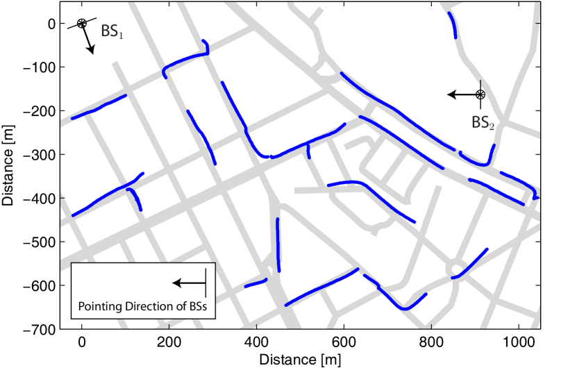
(a) Routes in Evaluation Scenario A.

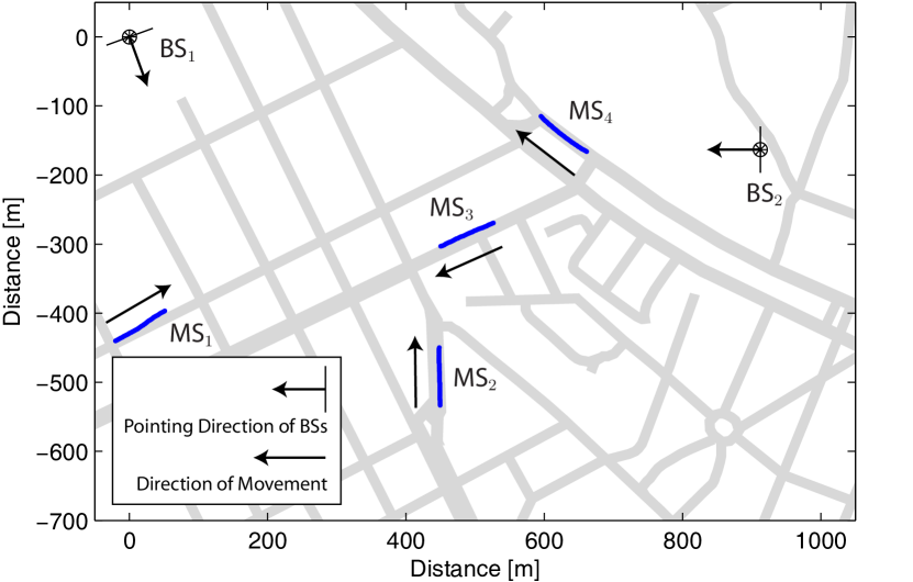
(b) Routes in Evaluation Scenario B.

Figure 2: Downlink evaluation based on measurements in an urban environment. Two four-antenna base stations are serving multiple single-antenna terminals. These terminals are either randomly located on the measured routes marked in Scenario A or move along fixed routes as in Scenario B.

The proposed CVSINR and DVSINR strategies are both suboptimal, but for a given subcarrier scheduling they can achieve asymptotic optimality in terms of multiplexing gain:

Theorem 4.

Let $\mathcal{S}_{c}\subseteq\{1,\ldots,K_{r}\}$ be the terminals scheduled for transmission on subcarrier $c$. If $|\mathcal{S}_{c}\cap\mathcal{C}_{j}|\leq N_{j}$ for all $j$ and $c$, then the CVSINR and DVSINR strategies achieve the multiplexing gain of $\sum_{c=1}^{K_{c}}|\mathcal{S}_{c}|$ (with probability one).

Proof:

The theorem follows by the same approach as in [Bjornson2010c, Theorem 5] and exploits that random channels are linearly independent with probability one. ∎

This means that the weighted sum rate behaves as $(\sum_{c=1}^{K_{c}}|\mathcal{S}_{c}|)\log_{2}(P)+\mathrm{constant}$ at high transmit power $P$. Thus, the absolute performance losses (also called power offsets) of the CVSINR and DVSINR strategies are bounded compared with the optimal solution, and the relative loss goes to zero as $\mathrm{constant}/\log_{2}(P)$ with increasing transmit power.

VI Measurement-Based Performance Evaluation

The theoretical performance of coordinated multicell transmission has been thoroughly studied for single- and multi-carrier systems (see e.g., [6, 12, Zheng2008a, Venturino2010a]). Under Rayleigh fading channels and perfect synchronization, large improvements over single-cell processing have been reported. Especially, cell edge terminals benefit from inter-cell interference coordination. However, results obtained from numerical simulations are highly dependent on the assumptions in the underlying channel models. For example, it is common to model the channel characteristics between a terminal and multiple base stations as uncorrelated, although correlation appears in practice [Jalden2007a]. Along with other idealized assumptions (e.g., on fading distributions and path losses), such channel dependencies may affect the performance of any multicell system.

The purpose of this section is to evaluate the performance of the low-complexity strategies in Section V on realistic multicell scenarios based on channel measurements. We only consider a single subcarrier for computationally reasons (the optimal solution to (P1) can be calculated systematically using [Bjornson2012a]) and since our measurements are flat-fading. However, the subcarriers in weighted sum rate optimization are only coupled by the power constraints and OFDMA systems are known for giving almost flat power allocation over subcarriers [Rhee2000a]. Thus, we expect our single-carrier results to be representative for general OFDMA systems.

The channel data was collected in Stockholm, Sweden, using two base stations with four-element uniform linear arrays (ULAs) with $0.56\lambda$ antenna spacing and one terminal. The terminal had a uniform circular array (UCA) with four directional antennas, but herein we average the signal over its antennas to create a single virtual omni-directional antenna. The system bandwidth was 9.6 kHz at a carrier frequency in the 1800 MHz band. The measurement environment can be characterized as typical European urban with four to six story high stone buildings. Fig. 2 shows the measurement area with roads illustrated in light gray and blue routes showing the GPS coordinates of the terminal locations used for the simulations herein. Further measurement details are available in [Jalden2007a]. The collected channel data is utilized to generate two evaluation scenarios where terminals are moving around in the area covered by both base stations:

• Scenario A: The performance behavior is evaluated over different random terminal distributions. In each snapshot, terminals can be located anywhere on the measured routes in Fig. 2(a) with uniform probability. To create balance, two terminals are placed to have their strongest channel gains ($\|\mathbf{h}_{jk}\|^{2}$) from $\textrm{BS}_{1}$, and the same for $\textrm{BS}_{2}$.

• Scenario B: To study the impact of coordination on individual terminals, four terminals are now placed at certain locations and moved as indicated in Fig. 2(b).

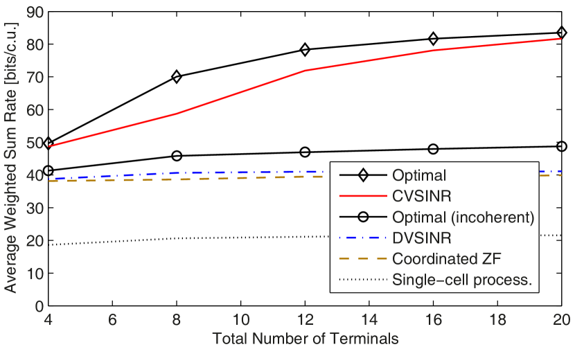
(a) 20 dBm output power per transmitter.

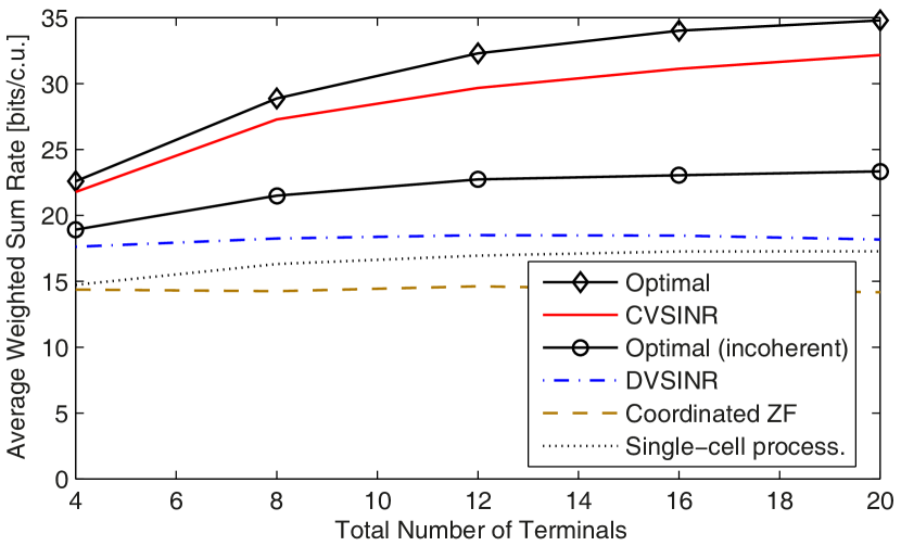
(b) 0 dBm output power per transmitter.

Figure 3: Average weighted sum rate (over random terminal locations) for Scenario A with different number of terminals. The performance is shown for different resource allocation strategies.

In both scenarios, the performance will be evaluated as a function of the output power per base station (in dBm). The noise level is set to $-131$ dBm (i.e., thermal noise and a few dBs of transmitter noise) and the measured path losses from the strongest base station varies between $-37$ dB and $-85$ dB for different terminal locations in Fig. 2.

The performance measure is the weighted sum rate with $\mu_{k}=c_{w}/\mathbb{E}\{\log_{2}(1+\frac{K_{t}}{K_{r}\sigma_{kc}^{2}}\max_{j}P_{j}\|\mathbf{h}_{jk}\|^{2})\}$, where $c_{w}$ is a scaling factor making $\sum_{k=1}^{K_{r}}\mu_{k}=K_{r}$. This represents proportional fairness (with equal power allocation). Six transmission strategies are compared:

1. The optimal solution (calculated using the framework in [Bjornson2012a] and using the optimization software CVX [cvx].).

2. The optimal solution under incoherent interference reception, where base stations cannot cancel out each other’s interference using joint transmission. This case is relevant since very tight synchronization and long cyclic prefixes are necessary to enable coherent interference cancelation over wide areas [Zhang2008a]. We represent it by replacing the SINR in (17) with

   $$\!\!\!\!\!\!\!\!\!\!\!\!\!\!\textrm{SINR}^{\textrm{DL-incoherent}}_{kc}=\frac{\big{|}{\underset{{j\in\mathcal{J}}}{\sum}}\sqrt{p_{jkc}}\mathbf{h}_{jkc}^{H}\mathbf{D}_{jk}\mathbf{v}_{jkc}\big{|}^{2}}{\sigma_{kc}^{2}\!+\!{\underset{{\bar{k}\in\mathcal{I}_{k}}}{\sum}}{\underset{{j\in\mathcal{J}}}{\sum}}\big{|}\sqrt{p_{j\bar{k}c}}\mathbf{h}_{jkc}^{H}\mathbf{C}_{jk}\mathbf{D}_{j\bar{k}}\mathbf{v}_{j\bar{k}c}\big{|}^{2}}.$$ (30)

3. Centralized virtual SINR (CVSINR) strategy, proposed in Section V-A.

4. Distributed virtual SINR (DVSINR) strategy, proposed in Section V-B.

5. Coordinated ZF precoding with single-cell scheduling using ProSched.

6. Single-cell processing as if there is only one cell in the system. The average out-of-cell interference is included in the $\sigma_{kc}^{2}$-terms. The resource allocation is based on the DVSINR strategy (pretending that $K_{t}=1$).

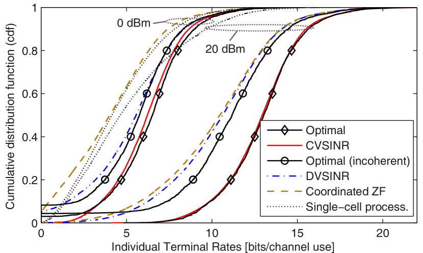
Figure 4: Cumulative distribution function of the individual terminal rates (over random terminal locations) for Scenario A with $K_{r}=4$. The performance is shown for different resource allocation strategies at 0 dBm and 20 dBm output power.

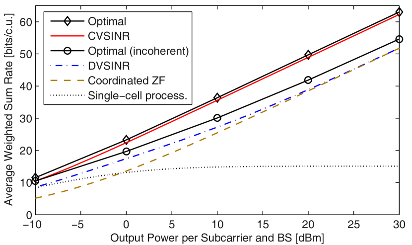
Figure 5: Average weighted sum rate as a function of the output power for Scenario B. The performance is shown for different resource allocation strategies, including the proposed CVSINR and DVSINR strategies.

VI-A Results for Evaluation Scenario A

The scheduling performance is evaluated in Fig. 3 over different random terminal locations, each used for 10 channel realizations. The average weighted sum rate is given as a function of the total number of terminals at 20 dBm and 0 dBm output power per transmitter. The proposed CVSINR strategy provides close-to-optimal performance, especially when the number of terminals increases. The gap to the optimal solution is remarkably small, given that CVSINR is a simple combination of ProSched scheduling and heuristic use of the optimality properties derived in Section IV—further parameter tweaking can certainly reduce the gap. The distributed strategies (DVSINR and coordinated ZF) stabilize on about half the performance of the centralized schemes, representing that only half the number of terminals can be simultaneously accommodated. One might think that this is due to that only one transmitter serves each terminal, but the actual explanation is that (non-iterative) distributed schemes cannot achieve coherent interference cancelation. This is understood by the comparably small difference from Strategy 2 which includes joint transmission but have incoherent interference reception, and it confirms the discussion in Section V-B. All the studied centralized and distributed strategies provide improvements over single-cell processing, and the differences increase rapidly with the output power.

Next, we want to study how multicell coordination impacts the performance of each terminal and we set $K_{r}=4$ to make sure that all six strategies consider the same set of terminals. In Fig. 4, the cumulative distribution functions (cdfs) of the individual terminal rates are given for output powers 0 dBm and 20 dBm. The proposed CVSINR strategy is very close to the optimal solution, in particular at high output power. The difference between the optimal solution and the DVSINR strategy increases with the SNR, but the distributed approach is close to the optimum under incoherent interference, which might be the most reasonable upper bound in practice [Zhang2008a]. Both CVSINR and DVSINR provide great improvements over single-cell processing—especially at high output power. The coordinated ZF scheme performs poorly at low output power, but approaches DVSINR at higher power. To summarize, terminals that move around in the cell clearly benefit from multicell coordination on the average through better statistical properties. In Scenario B, we will however see that terminals that are fixed at certain locations may experience performance degradations.

VI-B Results for Evaluation Scenario B

For Scenario B, the average weighted sum rate (per channel use and over 750 channel realizations) is shown in Fig. 5. Once again, the proposed CVSINR strategy provides close-to-optimal performance. As in Scenario A, there is a clear gap to the distributed approaches, explained by fewer degrees of freedom in the interference cancelation. However, both DVSINR and coordinated ZF achieve the maximal multiplexing gain in certain scenarios (see Theorem 4), while the performance of single-cell processing is bounded at high output power. Observe that the major gain over single-cell processing comes from interference cancelation for terminals in $\mathcal{C}_{j}$; the difference between DVSINR and optimal joint transmission is comparably small ($5-10$ dB).

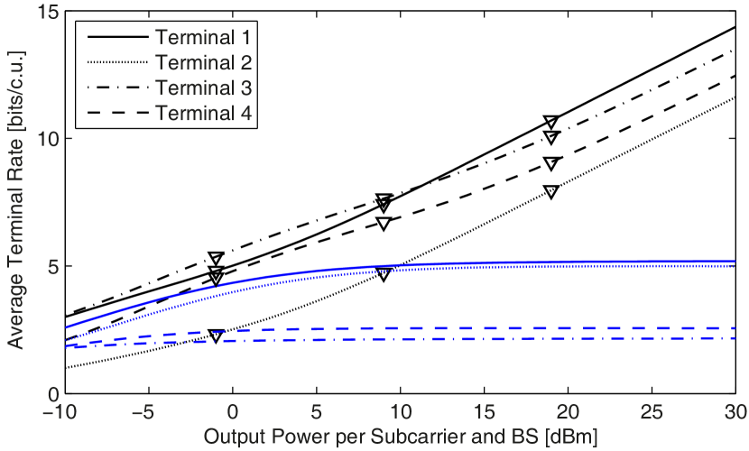
Figure 6: Average individual terminal rates for Scenario B with and without multicell coordination. The proposed DVSINR strategy (triangles) is compared with single-cell processing.

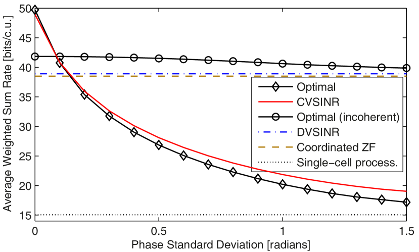
Figure 7: Weighted sum rate for Scenario B as a function of phase standard deviation $\sigma_{kc}$ (at 20 dBm output power). The actual channels are modeled as $\mathbf{h}_{jk}^{\textrm{actual}}=\mathbf{h}_{jk}e^{i\phi_{jk}}$, where $\phi_{jk}\in\mathcal{N}(0,\sigma_{\phi}^{2})$.

Fig. 6 shows the average individual terminal rates for DVSINR (marked with triangles) and single-cell processing. Interestingly, the increased weighted sum rate with multicell coordination does not translate into a monotonic improvement of all terminal rates. Terminal 3 has almost equally strong channels from both base stations and therefore gain substantially from interference coordination. However, Terminal 2 has a very weak link to $\textrm{BS}_{2}$ and sees a decrease in performance for output powers smaller than 10 dBm. This is explained by $\textrm{BS}_{1}$ modifying its precoding to avoid interference at Terminals 3 and 4. Thus, the common claim that multicell coordination improves both the total throughput and the fairness is not necessarily true in practice. However, Scenario A showed that as terminals move around in the whole area, they will on average benefit from multicell coordination.

The analysis has thus far considered perfect base station synchronization, which cannot be guaranteed in practice due to CSI uncertainty, hardware delays, clock drifts, insufficient cyclic prefixes, and minor channel changes. We emulate these mismatches by letting the actual channels be $\mathbf{h}_{jkc}^{\textrm{actual}}=\mathbf{h}_{jkc}e^{i\phi_{jkc}}$ for some random phase deviations $\phi_{jkc}\in\mathcal{N}(0,\sigma_{\phi}^{2})$ (where $\sigma_{\phi}=0$ means perfect synchronization). In Fig. 7, the average weighted sum rate is shown as a function of the phase standard deviation $\sigma_{\phi}$ (at 20 dBm output power). The optimal solution and the CVSINR strategy are very sensitive to synchronization errors as they rely on coherent interference cancelation where interfering signals from different base stations should cancel out perfectly. The DVSINR and coordinated ZF strategies are unaffected by such synchronization errors, and the gap to the optimal schemes based on incoherent interference reception reduces with $\sigma_{\phi}$. We conclude that very tight synchronization is required to gain from centralized multicell coordination with joint transmission.

VII Conclusion

A general multicell OFDMA resource allocation framework was introduced with dynamic cooperation clusters that enables unified analysis of anything from interference channels to ideal network MIMO. Joint precoding and scheduling optimization was considered using arbitrary monotonic utility functions and linear power constraints. This problem is typically non-convex and NP-hard, but we proved three properties of the optimal solution: 1) Optimality of single-stream beamforming; 2) Conditions for full power usage; and 3) A precoding parametrization based on $K_{r}K_{c}+L$ real-valued parameters between zero and one. These properties greatly reduces the search space for optimal resource allocation. To illustrate their usefulness, we proposed the centralized CVSINR strategy and the distributed DVSINR strategy. Both exploited the three optimality properties in conjunction with efficient ProSched subcarrier scheduling.

Contrary to previous work, the multicell performance was evaluated on measured channels in a typical urban macro-cell scenario. Substantial performance gains over single-cell processing were observed for both CVSINR and DVSINR. The former is even close-to-optimal, while the latter performs closely to what can be expected from distributed schemes (since coherent interference cancelation is more or less impossible to achieve). This is remarkable since both CVSINR and DVSINR are just simple applications of the derived optimality properties—further parameter tweaking and adaptation to special scenarios are possible. The performance evaluation also showed that joint transmission is very sensitive to synchronization errors and that multicell coordinated improves the average terminal performance, but that terminals in some parts of the cells can experience performance degradations.

Appendix A Proof of Lemma 4

Using Theorem 1, it is sufficient to consider solutions to (P2) of the form $\mathbf{S}_{kc}=\mathbf{w}_{kc}\mathbf{w}_{kc}^{H}$. Without loss of generality, we can select the phase of $\mathbf{w}_{kc}$ such that $\mathbf{h}_{kc}^{H}\mathbf{D}_{k}\mathbf{w}_{kc}>0$. Under these conditions, the feasibility problem (P2) can be expressed as

$$\begin{array}{cc}\hfill \underset{\{𝐰{}_{kc}\}{}_{k=1,c=1}{}^{K{}_r,K{}_c}}{\mathrm{minimize}}& \mathrm{\hspace{0.17em}\hspace{0.17em}0}\hfill \\ \hfill \mathrm{subject}\mathrm{to}& \sum {}_{k=1}{}^{K{}_r}\sum {}_{c=1}{}^{K{}_c}\mathrm{tr}\{𝐐{}_l𝐒{}_{kc}\}\le q{}_l\forall l,\hfill \\ & \parallel \hfill \\ \hfill \mathrm{⋮}\\ \hfill 𝐡{}_{kc}{}^H𝐂{}_k𝐃{}_{ℐ{}_k(|ℐ{}_k|)}𝐰{}_{ℐ{}_k(|ℐ{}_k|)c}\\ \hfill \sigma {}_{kc}\parallel \le \frac{𝐡{}_{kc}{}^H𝐃{}_k𝐰{}_{kc}}{\sqrt{\gamma {}_{kc}}}\forall k,c.& & & & \end{array}SincetheQoSconstraintsaresecondordercones,andthepowerconstraintsaresemi-definite,thisproblemisconvexandstrongdualityholds\text{<cite class="ltx\_cite ltx\_citemacro\_cite">[<span class="ltx\_ref ltx\_missing\_citation ltx\_ref\_self">Boyd2004a</span>]</cite>}.ToderivetheLagrangedualproblem,werewritetheLagrangianof(\text{<a href="\#A1.E37" title="In Appendix A Proof of Lemma 4 ‣ Optimality Properties, Distributed Strategies, and Measurement-Based Evaluation of Coordinated Multicell OFDMA Transmission" class="ltx\_ref ltx\_font\_italic"><span class="ltx\_text ltx\_ref\_tag">37</span></a>})similarlyto\text{<cite class="ltx\_cite ltx\_citemacro\_cite">[<span class="ltx\_ref ltx\_missing\_citation ltx\_ref\_self">Yu2007a</span>, Proposition 1]</cite>}:\text{(32)32L({wkc}k=1,c=1Kr,Kc,ω,{λc}c=1Kc)=(∑k=1Kr∑c=1Kcλkcσkc2-∑l=1Lωlql)+∑k=1Kr∑c=1KcwkcH(∑l=1LωlQl+¯k∈~Ik∑λ¯kcDkHC¯kHh¯kch¯kcHC¯kDk-λkcγkcDkHhkchkcHDk)wkc.}Minimizingwithrespectto\text{{ }\text{w}\text{\_kc }\_k=1,c=1^K\_r,K\_c}givesafinitesolutiononlyif\text{(33)33(∑l=1LωlQl+¯k∈~Ik∑λ¯kcDkHC¯kHh¯kch¯kcHC¯kDk-λkcγkcDkHhkchkcHDk)⪰0∀k,c,}andtheminimumisachievedby\text{w}\text{\_kc=}\text{0}.Using\text{<cite class="ltx\_cite ltx\_citemacro\_cite">[<span class="ltx\_ref ltx\_missing\_citation ltx\_ref\_self">Yu2007a</span>, Lemma 1]</cite>},thisdualfeasibilityconstraintcanberewrittenas\text{(34)34γkc≥λkchkcHDk(∑lωlQl+¯k∈~Ik∑λ¯kcDkHC¯kHh¯kch¯kcHC¯kDk-λkcγkcDkHhkchkcHDk)†DkHhkc=max¯wkcλkc¯wkcHDkHhkchkcHDk¯wkc¯wkcH(l∑ωlQl+¯k∈~Ik∑λ¯kcDkHC¯kHh¯kch¯kcHC¯kDk)¯wkc}wheretheequalityfollowsfromintroducingmaximizationoveranextravariable\overline{\text{w}}\text{\_kc ∈}\text{C}\text{^N ×1}.ObservethatthismaximizationcorrespondstoalinearMMSEreceiverwithoptimumat\text{(35)35¯wkc∗=λkc(∑l=1LωlQl+¯k∈~Ik∑λ¯kcDkHC¯kHh¯kch¯kcHC¯kDk)†DkHhkc.}Byplugging\text{w}\text{\_kc=}\text{0}into(\text{<a href="\#A1.E32" title="In 37 ‣ Appendix A Proof of Lemma 4 ‣ Optimality Properties, Distributed Strategies, and Measurement-Based Evaluation of Coordinated Multicell OFDMA Transmission" class="ltx\_ref ltx\_font\_italic"><span class="ltx\_text ltx\_ref\_tag">32</span></a>}),weachieveaLagrangedualproblemto(\text{<a href="\#A1.E37" title="In Appendix A Proof of Lemma 4 ‣ Optimality Properties, Distributed Strategies, and Measurement-Based Evaluation of Coordinated Multicell OFDMA Transmission" class="ltx\_ref ltx\_font\_italic"><span class="ltx\_text ltx\_ref\_tag">37</span></a>})and(\text{<a href="\#S3.Ex2" title="In III Problem Formulation ‣ Optimality Properties, Distributed Strategies, and Measurement-Based Evaluation of Coordinated Multicell OFDMA Transmission" class="ltx\_ref ltx\_font\_italic"><span class="ltx\_text ltx\_ref\_tag">P2</span></a>}):\begin{array}{cc}\hfill \underset{𝝎,\{𝝀{}_c\}{}_{c=1}{}^{K{}_c}}{\mathrm{maximize}}& \sum {}_{k=1}{}^{K{}_r}\sum {}_{c=1}{}^{K{}_c}\lambda {}_{kc}\sigma {}_{kc}{}^2-\sum {}_{l=1}{}^L\omega {}_{l}q{}_l\hfill \\ \hfill \mathrm{subject}\mathrm{to}& \lambda {}_{kc}\ge 0,\omega {}_l\ge 0\forall k,c,l,\hfill \\ & \max {}_{\overline{𝐰}{}_{kc}}\text{SINR}{}^{\text{VUL}}{}_{kc}(\overline{𝐰}{}_{1c},\mathrm{\dots },\overline{𝐰}{}_{K{}_{r}c},𝝎,𝝀{}_c)\le \gamma {}_{kc},\forall k,c.\hfill \end{array}Attheoptimum,allSINRconstraintsareactive(otherwisewecouldincreasesome\text{λ}\text{\_kc}andtherebyincreasethecostfunction),thuswereplacethemwithequalityconstraintsandachieve(\text{<a href="\#S4.Ex4" title="In Lemma 4. ‣ IV-C Parametrization of Optimal Precoding Strategies ‣ IV Properties of Optimal Resource Allocation ‣ Optimality Properties, Distributed Strategies, and Measurement-Based Evaluation of Coordinated Multicell OFDMA Transmission" class="ltx\_ref ltx\_font\_italic"><span class="ltx\_text ltx\_ref\_tag">D2</span></a>}).Finally,tofindarelationshipbetweenoptimal\overline{\text{w}}\text{\_kc}and\text{w}\text{\_kc}weconsiderthestationaryprincipleoftheLagrangianin(\text{<a href="\#A1.E32" title="In 37 ‣ Appendix A Proof of Lemma 4 ‣ Optimality Properties, Distributed Strategies, and Measurement-Based Evaluation of Coordinated Multicell OFDMA Transmission" class="ltx\_ref ltx\_font\_italic"><span class="ltx\_text ltx\_ref\_tag">32</span></a>}):\text{(36)360=∂L∂wkc=2(∑l=1LωlQl+¯k∈~Ik∑λ¯kcDkHC¯kHh¯kch¯kcHC¯kDk-λkcγkcDkHhkchkcHDk)wkc.}Bydefiningthescalar\text{d\_kc = }\text{λ}\text{\_kc }\text{h}\text{\_kc^H }\text{D}\text{\_k }\text{w}\text{\_kc /}\text{γ}\text{\_kc},weachieve\text{(37)37wkc=dkc(∑l=1LωlQl+¯k∈~Ik∑λ¯kcDkHC¯kHh¯kch¯kcHC¯kDk)†DkHhkc}andidentify\overline{\text{w}}\text{\_kc}from(\text{<a href="\#A1.E35" title="In 37 ‣ Appendix A Proof of Lemma 4 ‣ Optimality Properties, Distributed Strategies, and Measurement-Based Evaluation of Coordinated Multicell OFDMA Transmission" class="ltx\_ref ltx\_font\_italic"><span class="ltx\_text ltx\_ref\_tag">35</span></a>})(whichisuniqueuptoscaling).\text{Acknowledgement}TheauthorswouldliketothankDr.PerZetterbergforprovidingthechannelmeasurementsandforhisvaluableguidanceontheirdetails.\text{References[1]1}M.JiangandL.Hanzo,\mathrm{`}\mathrm{`}MultiuserMIMO-OFDMfornext-generationwirelesssystems,{}^{\prime \prime }\text{Proc. IEEE},vol.95,no.7,pp.1430--1469,2007.\text{[2]2}D.Gesbert,M.Kountouris,R.Heath,C.-B.Chae,andT.S\text{ä}lzer,\mathrm{`}\mathrm{`}ShiftingtheMIMOparadigm,{}^{\prime \prime }\text{IEEE Signal Process. Mag.},vol.24,no.5,pp.36--46,2007.\text{[3]3}S.Venkatesan,A.Lozano,andR.Valenzuela,\mathrm{`}\mathrm{`}NetworkMIMO:Overcomingintercellinterferenceinindoorwirelesssystems,{}^{\prime \prime }in\text{Proc. IEEE ACSSC’07},2007,pp.83--87.\text{[4]4}S.Parkvall,E.Dahlman,A.Furusk\text{ä}r,Y.Jading,M.Olsson,S.W\text{ä}nstedt,andK.Zangi,\mathrm{`}\mathrm{`}LTE-advanced-evolvingLTEtowardsIMT-advanced,{}^{\prime \prime }in\text{Proc. IEEE VTC’08-Fall},2008.\text{[5]5}S.ShamaiandB.Zaidel,\mathrm{`}\mathrm{`}Enhancingthecellulardownlinkcapacityviaco-processingatthetransmittingend,{}^{\prime \prime }in\text{Proc. IEEE VTC’01-Spring},vol.3,2001,pp.1745--1749.\text{[6]6}H.ZhangandH.Dai,\mathrm{`}\mathrm{`}CochannelinterferencemitigationandcooperativeprocessingindownlinkmulticellmultiuserMIMOnetworks,{}^{\prime \prime }\text{EURASIP J. Wirel. Commun. Netw.},vol.2,pp.222--235,2004.\text{[7]7}M.Karakayali,G.Foschini,andR.Valenzuela,\mathrm{`}\mathrm{`}Networkcoordinationforspectrallyefficientcommunicationsincellularsystems,{}^{\prime \prime }\text{IEEE Wireless Commun. Mag.},vol.13,no.4,pp.56--61,2006.\text{[8]8}H.Weingarten,Y.Steinberg,andS.Shamai,\mathrm{`}\mathrm{`}ThecapacityregionoftheGaussianmultiple-inputmultiple-outputbroadcastchannel,{}^{\prime \prime }\text{IEEE Trans. Inf. Theory},vol.52,no.9,pp.3936--3964,2006.\text{[9]9}P.MarschandG.Fettweis,\mathrm{`}\mathrm{`}Onmulticellcooperativetransmissioninbackhaul-constrainedcellularsystems,{}^{\prime \prime }\text{Ann. Telecommun.},vol.63,pp.253--269,2008.\text{[10]10}O.Simeone,O.Somekh,H.V.Poor,andS.Shamai,\mathrm{`}\mathrm{`}Downlinkmulticellprocessingwithlimited-backhaulcapacity,{}^{\prime \prime }\text{EURASIP J. on Adv. in Signal Process.},2009.\text{[11]11}E.Bj\text{ö}rnsonandB.Ottersten,\mathrm{`}\mathrm{`}Ontheprinciplesofmulticellprecodingwithcentralizedanddistributedcooperation,{}^{\prime \prime }in\text{Proc. WCSP’09},2009.\text{[12]12}A.T\text{ö}lli,M.Codreanu,andM.Juntti,\mathrm{`}\mathrm{`}CooperativeMIMO-OFDMcellularsystemwithsofthandoverbetweendistributedbasestationantennas,{}^{\prime \prime }\text{IEEE Trans. Wireless Commun.},vol.7,no.4,pp.1428--1440,2008.$$ (37)