Max-Planck Institut für Astrophysik, Karl-Schwarzschild-Straße 1, 85748, Garching, Germany
European Southern Observatory, Karl-Schwarzschild-Straße 2, 85748, Garching, Germany
Excellence Cluster Universe, Boltzmannstraße 2, 85748 Garching, Germany
School of Physics, University of Exeter, Stocker Road, Exeter EX4 4QL, UK
INAF-Osservatorio Astrofisico di Arcetri, Largo E. Fermi 5, I-50125 Firenze, Italy
Departamento de Física y Astronomía, Universidad de Valparaíso, Avda. Gran Bretaña 1111, Valparaiso, Chile
Can habitable planets form in clustered environments?
We present observational evidence of environmental effects on the formation and evolution of planetary systems. We combine catalogues of resolved protoplanetary discs (PPDs) and young stellar objects in the solar neighbourhood to analyse the PPD size distribution as a function of ambient stellar density. By running Kolmogorov-Smirnov tests between the PPD radii at different densities, we find empirical evidence, at the confidence level, for a change in the PPD radius distribution at ambient stellar densities . This coincides with a simple theoretical estimate for the truncation of PPDs or planetary systems by dynamical encounters. If this agreement is causal, the ongoing disruption of PPDs and planetary systems limits the possible existence of planets in the habitable zone, with shorter lifetimes at higher host stellar masses and ambient densities. Therefore, habitable planets are not likely to be present in long-lived stellar clusters, and may have been ejected altogether to form a population of unbound, free-floating planets. We conclude that, while highly suggestive, our results should be verified through other methods. Our simple model shows that truncations should lead to a measurable depletion of the PPD mass function that can be detected with ALMA observations of the densest nearby and young clusters.
Key Words.:
Planets and satellites: formation – Protoplanetary disks – (Stars:) circumstellar matter – Stars: kinematics and dynamics – (Galaxy:) open clusters and associations: general1 Introduction
For the past decade, exoplanetary systems are being discovered at a spectacular rate (e.g. Mayor et al. 2004; Borucki et al. 2011). Driven by these discoveries, there is an increasing interest in the global properties of planetary systems, from the epoch of their formation in protoplanetary discs (PPDs) to their long-term stability. While there is a natural focus on internal processes that govern the evolution of such systems (e.g. Lee & Peale 2003; Dullemond & Dominik 2005; Gorti et al. 2009; Morbidelli et al. 2009; Brasser et al. 2009; Blum 2010; Williams & Cieza 2011), it is clear that not all planetary systems form in isolation and environmental effects should be considered as well. Particularly, theoretical studies show that external photoevaporation (Scally & Clarke 2001; Adams et al. 2004, 2006; Fatuzzo & Adams 2008) and dynamical interactions (Bonnell et al. 2001; Pfalzner et al. 2005; Olczak et al. 2006, 2010; Spurzem et al. 2009; Lestrade et al. 2011; Dukes & Krumholz 2012; Parker & Quanz 2012; Bate 2012) can lead to the truncation of PPDs and planetary systems.
While the external photoevaporation of PPDs has been studied observationally (O’dell et al. 1993; Robberto et al. 2008; Rigliaco et al. 2009; Mann & Williams 2010), there is no conclusive evidence of dynamical effects (Eisner & Carpenter 2006; Olczak et al. 2008; Reche et al. 2009). In part, this is likely due to the relatively short lifetimes of PPDs (up to Myr, e.g. Haisch et al. 2001; Hernández et al. 2008; Ercolano et al. 2011; Smith & Jeffries 2012) compared to the time it takes stellar encounters to have an observable effect on the disc population (– Gyr, e.g. Adams 2010). Previous observational studies on the Orion Nebula Cluster (ONC) (e.g. Eisner & Carpenter 2006; Olczak et al. 2008) did aim to find traces of dynamical interactions in the population of PPDs, but lacked a sufficient number of sources and/or suffered from uncertainties on the disc mass measurements.
We address the problem statistically by considering the sizes of PPDs as a function of their ambient stellar density, using samples of PPDs and young stellar objects (YSOs) from the latest infrared surveys. If stellar encounters truncate PPDs by tidally stripping the outskirts of the discs (e.g. Clarke & Pringle 1993; Heller 1995; Hall et al. 1996), this should be observable above some characteristic ambient stellar density ( Adams 2010), because the encounter rate increases with density (e.g. Binney & Tremaine 1987, Eq. 7-61). In this Letter, we find model-independent evidence of a change in the PPD size distribution for ambient stellar surface densities at the confidence level.
2 Protoplanetary discs and their environment
2.1 Data selection
To verify whether a relationship exists between the sizes of PPDs and their ambient stellar surface density, , we combine existing catalogues of PPDs and young stellar objects in star-forming regions (SFRs) of the solar neighbourhood.
The data for the PPDs is taken from circumstellardisks.org (Karl Stapelfeldt, NASA/JPL). This catalogue gathers resolved PPDs that have been confirmed and described in the literature. If a PPD is resolved in different wavelengths (probing different parts of the disc, see e.g. Lada et al. 2006), the catalogue lists the largest measured diameter, implying that the disc radii used in this work are lower limits. About of the PPD radii in our final sample (see below) are measured at wavelengths around , with only of the PPDs (all in low-density regions) being observed at mm wavelengths (see Appendix A). The catalogue contains an estimate for how well-resolved each disc is by listing the number of diffraction-limited beams that fit within its diameter. We only consider the discs for which this value is greater than unity. This provides us with PPD sources from which we exclude those whose host star is classified as a main sequence star, weak-line T-Tauri star, or Class 0 YSO. Sources at distances pc (which covers all our YSOs) are also excluded. These criteria reduce the sample to a total of sources.
To estimate the local ambient surface density of each PPD source, we use publicly available near-infrared data of nearby SFRs (see Table 2 in Appendix A). The ambient surface density of stars around each PPD is estimated as in Casertano & Hut (1985) – see Appendix A for a detailed explanation. The thus-obtained angular ambient surface densities are converted to physical ambient stellar surface densities, , using the distances listed in Table 2. In cases where the listed PPD distance differs from the distance to the region that it is a member of, we adjust the PPD distance and size. Since a low surface density can be due to incomplete YSO coverage, any discs with are omitted from our analysis. Moreover, the minimum PPD radius that can be resolved increases with distance and hence introduces a distance-dependent selection bias. To avoid this, we exclude any PPDs smaller than the smallest radius ( AU) that is resolved in the most distant region of our sample, which is the Orion Nebula Cluster (ONC). The final sample thus contains sources (see Table 1 in Appendix A). Completeness does not affect the densities because the surveys of Table 2 are complete down to the hydrogen-burning limit.
2.2 A simple theoretical estimate for the truncation of discs
To interpret the data, we include a rough theoretical estimate for the expected truncation radii of PPDs as a function of . This is obtained by combining the truncation induced by each particular encounter with the stellar encounter rate. The derivation is presented in detail in Appendix B.
We use the numerical simulations of disc perturbations in clustered environments by Olczak et al. (2006) to obtain the disc radius as a function of the encounter parameters. We convert their expressions for the disc mass loss to a radial truncation assuming that it occurs by stripping the outer disc layers to the Lagrangian point between both stars, and adopting a PPD surface density profile (Olczak et al. 2006). Under these assumptions, we write for the upper limit to the disc radius
| (1) |
where is the pericentre radius at which the perturber passes, the mass of the perturbed system, and the mass of the perturber. This approximation is validated in Appendix B.
The encounter radius is obtained from the impact parameter , encounter velocity , and masses and by accounting for gravitational focussing (see Appendix B). The masses are assumed to follow a Salpeter (1955) type initial mass function in the range 0.1–100 M⊙, and the velocity distribution is taken to be Maxwellian with a velocity dispersion of km s-1, as is typical for SFRs (Hillenbrand & Hartmann 1998; Covey et al. 2006). This enables the derivation of the encounter rate as a function of and (Binney & Tremaine 1987), which for a given age provides the total number of encounters . Because encounters with pericentres at inclination angles with respect to the disc plane affect the disc only mildly, about of the encounters lead to the disc truncation described by Eq. 1 (Pfalzner et al. 2005). We use the probability distribution functions (PDFs) for , , and to calculate the PDF of the ‘most disruptive’ encounter, i.e. the parameter set that gives the smallest disc size, according to Maschberger & Clarke (2008, Eq. A5). We then integrate the product of the disc radius , the PDF of the ‘most disruptive encounter’, and the mass PDF of the perturbed object to obtain the expected disc truncation radius . To compare the theoretical estimate to the observations, we relate the stellar volume density to the surface density as , where pc is a typical radius for the SFRs in our sample (Hillenbrand & Hartmann 1998; Evans et al. 2009).
3 Results
3.1 Evidence for environmental effects
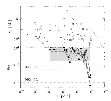
The upper panel of Fig. 1 shows the observed PPD radii versus . The distribution is relatively insensitive to the ambient density until , where it appears truncated at large radii. This is consistent with the simple theoretical approximation from Sect. 2.2, which predicts a truncation at these densities for ages between and Myr (see Fig. 1). The affected PPDs are all in the ONC. If the truncation is interpreted as being due to dynamical interactions, the theoretical curves suggest that youngest sources in the ONC have ages of Myr, which is reasonably consistent with observations (Palla & Stahler 1999; Da Rio et al. 2010; Jeffries et al. 2011). However, this is not a unique explanation, since the truncation might also be due to external photoevaporation by nearby massive stars (e.g. Clarke 2007). It is also important to keep in mind that some fraction of the PPDs at this projected surface density will actually reside in a region of lower volume density, either behind or in front of the high-density core of the ONC. The distribution also shows some evidence of a density-independent upper limit to the PPD radius of AU, which could be related to binarity (Artymowicz & Lubow 1994; Kraus et al. 2012) or be intrinsic (Basu 1998).
To test the statistical significance of the change in the radius distribution, we perform a Kolmogrov-Smirnov (KS) test, which is theory-independent and thus insensitive to model assumptions. It gives the probability that two samples were drawn from the same parent distribution. Starting at the high-density end, we first divide the sample in density bins of objects per bin, which represents a balance between good statistics and enough bins to resolve the regime where the radius distribution changes. The KS test is then carried out comparing radii in a bin at density with those at lower densities (i.e. ). We do not include bins at to avoid low-number statistics in the reference sample. The bottom panel of Fig. 1 shows the results of the test. At intermediate densities, all KS tests give high -values, but for densities higher than there is a pronounced drop. As such, the KS test yields a detection of a change in the PPD radius distribution at the confidence level. Note that this does not change when excluding the largest PPD in the sample (at ). The result also holds within the ONC only (grey line in Fig. 1), when dividing the ONC subsample in two at each density and running a KS test for the radii at both sides of the separation. To check the result, we performed 30,000 Monte Carlo experiments in which the KS test was applied in the same way to distributions of randomly paired radii and surface densities, i.e. erasing any possible correlation. Figure 1 indicates the resulting median and its dispersion, showing that the results obtained for the original sample are unlikely to be due to the adopted statistical method.
3.2 Implications for habitable zone occupancy lifetimes

If the drop of the -value at high densities is indeed caused by dynamical truncation, then the model can be used to give the maximum time during which the habitable zone (HZ) can host a planet or a PPD (‘HZ lifetime’). We calculate as a function of and as in Fig. 1, but without averaging over the host stellar mass to retain the mass dependence. We then compare it to the inner radius of the HZ, , and determine until which age they overlap, as a function of mass and ambient density. The radius depends on the required radiative equilibrium temperature , on the stellar luminosity and on the properties of the planet (i.e. , a proxy for atmospheric thermal circulation, and the Bond albedo , see Kasting et al. 1993; Tarter et al. 2007):
| (2) |
where is the Stefan-Boltzman constant. Following Borucki et al. (2011), we calculate for an Earth-like planet using , , and , which is the maximum temperature that allows for the presence of liquid water when accounting for the greenhouse effect. The luminosity is taken from stellar evolution models at solar metallicity (Marigo et al. 2008). The results are shown in Figure 2 for ambient densities of . The HZ lifetime decreases with density and stellar mass, due to the enhanced encounter rate and the large , respectively. These estimates for the HZ lifetime hold both for PPDs and planetary systems, since dynamical interactions would have comparable effects in both cases (e.g. Olczak et al. 2006; Parker & Quanz 2012).
Figure 2 shows that, based on the Earth’s existence alone, the solar system cannot have formed in a dense () environment, unless the ambient density decreased on a short ( Myr) timescale. Conversely, meteoritic evidence indicates that the young solar system must have endured nearby supernovae (e.g. Cameron & Truran 1977), which provides a lower limit to the product (see the review by Adams 2010). A plausible scenario is thus that the solar system formed in a massive (, ), but unbound association, which dispersed on a short ( Myr) timescale (see e.g. Dukes & Krumholz 2012, although they refer to such a system as a ‘cluster’). Our results seem to disagree with Eisner & Carpenter (2006) who derive the disc fraction in the ONC and find no evidence of disc truncations. However, their conclusion may result from low-number statistics, and PPD mass estimates are more uncertain than radius measurements. On the other hand, our results agree with the studies of Bonnell et al. (2001) and Spurzem et al. (2009), and would explain why no planets have been found in the globular clusters 47 Tuc and NGC 6397 (Gilliland et al. 2000; Nascimbeni et al. 2012), where within the half-mass radius. This implies such a high number of encounters that it is improbable that any bound planets survived, most of them likely to have escaped the cluster due to two-body relaxation (e.g. Kruijssen 2009).
We note that our theoretical estimates are conservative and provide upper limits to the disc sizes, because (1) we do not account for potentially higher ambient densities in the past (e.g. Bastian et al. 2008), (2) we neglect the presence of massive stars at earlier ages of the SFRs, (3) we only consider the most disruptive encounters and ignore the cumulative effect of weak perturbations. Figure 2 thus provides strict upper limits to the HZ lifetimes.
4 Further observational avenues
We present evidence for a change in the PPD radius distribution at ambient stellar densities of at the confidence level, in line with the expected range due to close encounters with other stars on a Myr timescale. These densities are only reached in the densest parts of the ONC, which is not only consistent with the detection of reduced PPD masses in the centre of the region (Mann & Williams 2010), but also with studies concluding that encounters are not important in the ONC as a whole (e.g. Scally & Clarke 2001). Our results demonstrate that the stellar environment can be an important factor in setting the habitability of planetary systems. For instance, the existence of unbound, free-floating planets (see e.g. Bihain et al. 2009; Sumi et al. 2011; Strigari et al. 2012) is a natural outcome of our results. However, a ubiquity of Earth-like planets in the HZ of stars remains likely because a large fraction () of stars forms in unbound associations (see Kruijssen 2012 for a recent review, and observational references therein), of which the density quickly decreases after their formation.

To verify our results, more observations of PPDs in clustered environments are desirable. A fruitful approach would be to probe PPD truncations using disc mass measurements, which would provide much larger samples of PPDs. Figure 3 shows the effect of (only) dynamical encounters on the disc mass function (DMF) using the disc mass loss description from Olczak et al. (2006) (see Appendix C). This will be easily observable in dense and young stellar clusters with ALMA. While the full ALMA array will be able to directly measure disc sizes, we predict that, already from Early Science Cycle 1, the sensitivity will be sufficient to detect the variation of the DMF caused by the truncation (see Fig. 3), which would verify the result of Fig. 1.
Acknowledgements.
We are grateful to the anonymous referee for a thoughtful and constructive report. We thank Cathie Clarke, Michael Meyer, and Christoph Olczak for insightful comments on the manuscript, and David Jewitt, Thomas Maschberger, and Niels Oppermann for helpful discussions. NB is supported by the DFG cluster of excellence ‘Origin and Structure of the Universe’ and HC by the Millennium Science Initiative, Chilean Ministry of Economy, Nucleus P10-022-F.References
- Adams (2010) Adams, F. C. 2010, ARA&A, 48, 47
- Adams et al. (2004) Adams, F. C., Hollenbach, D., Laughlin, G., & Gorti, U. 2004, ApJ, 611, 360
- Adams et al. (2006) Adams, F. C., Proszkow, E. M., Fatuzzo, M., & Myers, P. C. 2006, ApJ, 641, 504
- Andrews & Williams (2005) Andrews, S. M. & Williams, J. P. 2005, ApJ, 631, 1134
- Artymowicz & Lubow (1994) Artymowicz, P. & Lubow, S. H. 1994, ApJ, 421, 651
- Bastian et al. (2008) Bastian, N., Gieles, M., Goodwin, S. P., et al. 2008, MNRAS, 389, 223
- Basu (1998) Basu, S. 1998, ApJ, 509, 229
- Bate (2012) Bate, M. R. 2012, MNRAS, 419, 3115
- Bihain et al. (2009) Bihain, G., Rebolo, R., Zapatero Osorio, M. R., et al. 2009, A&A, 506, 1169
- Binney & Tremaine (1987) Binney, J. & Tremaine, S. 1987, Galactic dynamics (Princeton, NJ, Princeton University Press, 1987, 747 pp.)
- Blum (2010) Blum, J. 2010, Research in Astronomy and Astrophysics, 10, 1199
- Bonnell et al. (2001) Bonnell, I. A., Smith, K. W., Davies, M. B., & Horne, K. 2001, MNRAS, 322, 859
- Borucki et al. (2011) Borucki, W. J., Koch, D. G., Basri, G., et al. 2011, ApJ, 736, 19
- Brasser et al. (2009) Brasser, R., Morbidelli, A., Gomes, R., Tsiganis, K., & Levison, H. F. 2009, A&A, 507, 1053
- Bressert et al. (2010) Bressert, E., Bastian, N., Gutermuth, R., et al. 2010, MNRAS, 409, L54
- Cameron & Truran (1977) Cameron, A. G. W. & Truran, J. W. 1977, Icarus, 30, 447
- Casertano & Hut (1985) Casertano, S. & Hut, P. 1985, ApJ, 298, 80
- Clarke (2007) Clarke, C. J. 2007, MNRAS, 376, 1350
- Clarke & Pringle (1993) Clarke, C. J. & Pringle, J. E. 1993, MNRAS, 261, 190
- Covey et al. (2006) Covey, K. R., Greene, T. P., Doppmann, G. W., & Lada, C. J. 2006, AJ, 131, 512
- Da Rio et al. (2010) Da Rio, N., Robberto, M., Soderblom, D. R., et al. 2010, ApJ, 722, 1092
- Dukes & Krumholz (2012) Dukes, D. & Krumholz, M. R. 2012, ApJ, 754, 56
- Dullemond & Dominik (2005) Dullemond, C. P. & Dominik, C. 2005, A&A, 434, 971
- Eisner & Carpenter (2006) Eisner, J. A. & Carpenter, J. M. 2006, ApJ, 641, 1162
- Ercolano et al. (2011) Ercolano, B., Bastian, N., Spezzi, L., & Owen, J. 2011, MNRAS, 416, 439
- Evans et al. (2003) Evans, II, N. J., Allen, L. E., Blake, G. A., et al. 2003, PASP, 115, 965
- Evans et al. (2009) Evans, II, N. J., Dunham, M. M., Jørgensen, J. K., et al. 2009, ApJS, 181, 321
- Fatuzzo & Adams (2008) Fatuzzo, M. & Adams, F. C. 2008, ApJ, 675, 1361
- Gilliland et al. (2000) Gilliland, R. L., Brown, T. M., Guhathakurta, P., et al. 2000, ApJ, 545, L47
- Gorti et al. (2009) Gorti, U., Dullemond, C. P., & Hollenbach, D. 2009, ApJ, 705, 1237
- Haisch et al. (2001) Haisch, Jr., K. E., Lada, E. A., & Lada, C. J. 2001, ApJ, 553, L153
- Hall et al. (1996) Hall, S. M., Clarke, C. J., & Pringle, J. E. 1996, MNRAS, 278, 303
- Heller (1995) Heller, C. H. 1995, ApJ, 455, 252
- Hernández et al. (2008) Hernández, J., Hartmann, L., Calvet, N., et al. 2008, ApJ, 686, 1195
- Hillenbrand & Hartmann (1998) Hillenbrand, L. A. & Hartmann, L. W. 1998, ApJ, 492, 540
- Jeffries et al. (2011) Jeffries, R. D., Littlefair, S. P., Naylor, T., & Mayne, N. J. 2011, MNRAS, 418, 1948
- Kasting et al. (1993) Kasting, J. F., Whitmire, D. P., & Reynolds, R. T. 1993, Icarus, 101, 108
- Kraus et al. (2012) Kraus, A. L., Ireland, M. J., Hillenbrand, L. A., & Martinache, F. 2012, ApJ, 745, 19
- Kruijssen (2009) Kruijssen, J. M. D. 2009, A&A, 507, 1409
- Kruijssen (2012) Kruijssen, J. M. D. 2012, MNRAS in press, arXiv:1208.2963
- Lada et al. (2006) Lada, C. J., Muench, A. A., Luhman, K. L., et al. 2006, AJ, 131, 1574
- Lee & Peale (2003) Lee, M. H. & Peale, S. J. 2003, ApJ, 592, 1201
- Lestrade et al. (2011) Lestrade, J.-F., Morey, E., Lassus, A., & Phou, N. 2011, A&A, 532, A120
- Mann & Williams (2010) Mann, R. K. & Williams, J. P. 2010, ApJ, 725, 430
- Marigo et al. (2008) Marigo, P., Girardi, L., Bressan, A., et al. 2008, A&A, 482, 883
- Maschberger & Clarke (2008) Maschberger, T. & Clarke, C. J. 2008, MNRAS, 391, 711
- Mayor et al. (2004) Mayor, M., Udry, S., Naef, D., et al. 2004, A&A, 415, 391
- Morbidelli et al. (2009) Morbidelli, A., Brasser, R., Tsiganis, K., Gomes, R., & Levison, H. F. 2009, A&A, 507, 1041
- Nascimbeni et al. (2012) Nascimbeni, V., Bedin, L. R., Piotto, G., De Marchi, F., & Rich, R. M. 2012, A&A, 541, A144
- O’dell et al. (1993) O’dell, C. R., Wen, Z., & Hu, X. 1993, ApJ, 410, 696
- Olczak et al. (2008) Olczak, C., Pfalzner, S., & Eckart, A. 2008, A&A, 488, 191
- Olczak et al. (2010) Olczak, C., Pfalzner, S., & Eckart, A. 2010, A&A, 509, A63
- Olczak et al. (2006) Olczak, C., Pfalzner, S., & Spurzem, R. 2006, ApJ, 642, 1140
- Palla & Stahler (1999) Palla, F. & Stahler, S. W. 1999, ApJ, 525, 772
- Parker & Quanz (2012) Parker, R. J. & Quanz, S. P. 2012, MNRAS, 419, 2448
- Pfalzner et al. (2005) Pfalzner, S., Vogel, P., Scharwächter, J., & Olczak, C. 2005, A&A, 437, 967
- Rebull et al. (2010) Rebull, L. M., Padgett, D. L., McCabe, C.-E., et al. 2010, ApJS, 186, 259
- Reche et al. (2009) Reche, R., Beust, H., & Augereau, J.-C. 2009, A&A, 493, 661
- Rigliaco et al. (2009) Rigliaco, E., Natta, A., Randich, S., & Sacco, G. 2009, A&A, 495, L13
- Robberto et al. (2008) Robberto, M., Ricci, L., Da Rio, N., & Soderblom, D. R. 2008, ApJ, 687, L83
- Robberto et al. (2010) Robberto, M., Soderblom, D. R., Scandariato, G., et al. 2010, AJ, 139, 950
- Salpeter (1955) Salpeter, E. E. 1955, ApJ, 121, 161
- Scally & Clarke (2001) Scally, A. & Clarke, C. 2001, MNRAS, 325, 449
- Smith & Jeffries (2012) Smith, R. & Jeffries, R. D. 2012, MNRAS, 420, 2884
- Spurzem et al. (2009) Spurzem, R., Giersz, M., Heggie, D. C., & Lin, D. N. C. 2009, ApJ, 697, 458
- Strigari et al. (2012) Strigari, L. E., Barnabè, M., Marshall, P. J., & Blandford, R. D. 2012, MNRAS, 423, 1856
- Sumi et al. (2011) Sumi, T., Kamiya, K., Bennett, D. P., et al. 2011, Nature, 473, 349
- Tarter et al. (2007) Tarter, J. C., Backus, P. R., Mancinelli, R. L., et al. 2007, Astrobiology, 7, 30
- Williams & Cieza (2011) Williams, J. P. & Cieza, L. A. 2011, ARA&A, 49, 67
Appendix A Properties of the sample
| Type | Sources | KS |
|---|---|---|
| Herbig Ae or Be | 15 | 3 |
| T-Tauri | 39 | 21 |
| Unknown central star (ONC) | 36 | 35 |
| Young stellar object | 11 | 8 |
After the selection procedure detailed in Sect. 2.1, we list the final PPD sample in Table 1. To assess the heterogeneity of the sample, we show the wavelengths of the radius measurements as a function of ambient stellar density in Fig. 4. The vast majority of sources () were measured in a narrow wavelength range below (i.e near infrared wavelengths) with a spread of and centred at . The remaining sources were measured at millimetre wavelengths. For the ONC sample, of all sources were measured at with very little scatter overall. As shown in Fig. 4, the sources of the total sample measured at millimetre wavelengths all have ambient surface stellar density . Therefore the distribution at densities above this value can be considered to be homogeneous.

| Name | (pc) | Survey | |
|---|---|---|---|
| Lupus I | 20 | 150 | 1 |
| Lupus III | 79 | 150 | 1 |
| Lupus IV | 12 | 150 | 1 |
| Ophiuchus | 297 | 125 | 1 |
| Orion Nebula Cluster | 7759 | 414 | 3 |
| Perseus | 387 | 250 | 1 |
| Serpens | 262 | 415 | 1 |
| Taurus | 249 | 137 | 2 |
The regions from which the YSOs are taken to estimate the ambient density are summarized in Table 2. Using these samples, the ambient surface density of stars around each PPD is estimated as (Casertano & Hut 1985):
| (3) |
where is the rank of the th nearest neighbour, and is the projected angular distance to that neighbour. We use , which is higher than the commonly-used value of (cf. Bressert et al. 2010) and is chosen to improve the statistics of the density estimates. An additional effect of using a higher value of is a slight decrease of the density estimates. This should be kept in mind when comparing our densities those in other work.
Appendix B A simple model for PPD truncations
In this Appendix, we derive the upper limit to the radii of protoplanetary discs (PPDs) due to dynamical encounters. Where appropriate, we emphasize that the derivation is conservative, such that the obtained truncation radius is indeed an upper limit.
Olczak et al. (2006) performed numerical simulations of disc perturbations and provided an expression for the relative disc mass loss due to encounters with other stars (their Eq. 4). If we assume that the mass loss occurs by stripping the outer disc layers and adopt the disc surface density profile of used in their work, then . The expression for from Olczak et al. (2006) is consistent to within a factor of three with the scenario in which a disc is always truncated to the equipotential (Lagrangian) point between both stars. If the disc was already smaller than that radius, it is left relatively unperturbed. For the rough estimate made here, it thus suffices to write for the upper limit to the disc radius
| (4) |
where is the pericentre radius at which the perturber passes, is the mass of the perturbed system and is the mass of the perturber. The approximation of Eq. 4 follows Eq. 4 of Olczak et al. (2006) with reasonable accuracy for initial disc radii up to a few AU (consistent with the parameter space in Fig. 1), encounter distances pc (i.e. ) and mass ratios . We have verified that these conditions are satisfied for the encounters that are expected to determine the disc truncation (see below). Following Binney & Tremaine (1987), the impact parameter and the encounter radius due to gravitational focusing are related as
| (5) |
where is the relative velocity of the encounter. This equation is inverted to derive for each encounter.
The truncation radius of Eq. 4 depends on the variable set , for which we specify probability distribution functions (PDFs). For the masses, we use a Salpeter (1955) type initial mass function in the range 0.1 M⊙–, where depends on age due to stellar evolution. For ages Myr we assume , while at later ages it is set by the Marigo et al. (2008) stellar evolution models at solar metallicity. The mass function is:
| (6) |
which is normalized such that . Assuming a Maxwellian velocity distribution, the total number of encounters per unit velocity and unit impact parameter follows from the encounter rate as (Binney & Tremaine 1987)
| (7) |
where is the local number density of stars, is the age of the region, and is the velocity dispersion. The relative velocity ranges from – and the impact parameter from – (see below). As in Eq. 6, we have normalized such that , by writing and defining as the total number of encounters at age . The factor represents the fraction of encounters that leads to disc mass loss according to Eq. 4. This accounts for the fact that encounters with pericentres at inclination angles with respect to the disc plane cause only weak mass loss and retrograde encounters leave the disc almost unperturbed (Pfalzner et al. 2005).
Given a sequence of encounters, the truncation of the PPD is set by the most disruptive encounter (Scally & Clarke 2001, although see Olczak et al. 2006), i.e. . If we assume that are uncorrelated, implying that the region is not mass-segregated, the PDF of the most disruptive encounter becomes
| (8) |
where represent the PDFs for the lowest , lowest and highest , respectively. Following the method of Maschberger & Clarke (2008, Eq. A5), these three PDFs are defined as
| (9) | |||||
where are the distribution functions for and , with and , again normalized to unity in both cases. In Eqs. B, , and indicate variable limits, and and indicate fixed limits. The fixed limit represents the maximum impact parameter, which is given by the typical interstellar separation (the factor was chosen for consistency with Scally & Clarke 2001). It should be noted that while this is a physically motivated choice, it only weakly influences the result since the most likely most disruptive encounter will typically be at . Assuming an age of Myr, for surface densities of stars pc-2 we find that always peaks at impact parameters pc (i.e. ), whereas for pc-2 the most likely most disruptive encounter always has , which after averaging over the mass function to account for the distribution of gives . This validates the use of the approximation in Eq. 4.
By combining the Eqs. 6 and 8, the total PDF is
| (10) |
It should be noted that we did not include the mass of the perturbed object in the PDF of the most likely most disruptive encounter (Eq. 8), but instead average over the mass PDF itself. The reason is that the stars in Fig. 1 span a range of masses, and a ‘typical’ relation between the truncation radius and ambient density is preferable.
Combining the previous equations gives a theoretical estimate for the typical truncation radius as a function of the ambient density, velocity dispersion and age:
| (11) |
where indicates the complete phase space, i.e. 0.1 M⊙– in mass, 0– in velocity and 0– in impact parameter. This expression provides the expected radius after the ‘most likely most disruptive encounter’, averaged over the stellar mass function to account for the unknown mass of the perturbed system.
Appendix C Evolution of the disc mass function
To calculate the evolution of the disc mass function (DMF), we assume that the initial disc mass is related to the host stellar mass as
| (12) |
where is a constant. We adopt , which is in good agreement with observations (Andrews & Williams 2005) and sufficiently accurate for the order-of-magnitude estimate made in Sect. 4. Using a Salpeter (1955) stellar initial mass function (cf. Eq. 6), the initial DMF is
| (13) |
For each host stellar mass, we calculate the characteristics of the most likely most disruptive encounter as in Appendix B, using quantities that are appropriate for NGC 3603 (i.e. Myr, , and pc). Given a certain encounter, the disc mass loss is calculated using the expression from Olczak et al. (2006, Eq. 4), which provides as a function of the host stellar mass , the mass of the perturber , the pericentre distance and the disc radius . To account for the dependence of on the radius, it is calculated for all radii from the observed sample at ambient densities (see Fig. 1), including those with AU since the corresponding regions are all nearby and hence the detection limit is less stringent. At these densities the encounter rate is so low that the observed disc radii can be interpreted as ‘initial’ radii. The obtained values of are then averaged to remove the dependence on , and integrated (see Eq. 10) in the same way as in Eq. 11. This provides the expected relative mass loss as a function of host stellar mass ,111Note that contrary to our Lagrangian approximation of Eq. 4, the disc mass loss of the Olczak et al. (2006) equation does not increase monotonically with decreasing pericentre distance – for very close encounters (typically ) the disc mass loss is reduced. In such cases, the most disruptive encounter is not the closest encounter, and we account for this by adjusting to the value where peaks. and hence the final disc mass is approximately
| (14) |
The final DMF is then given by
| (15) | |||||