Ion chains in high-finesse cavities

Abstract

We analyze the dynamics of a chain of singly-charged ions confined in a linear Paul trap and which couple with the mode of a high-finesse optical resonator. In these settings the ions interact via the Coulomb repulsion and are subject to the mechanical forces due to scattering of cavity photons. We show that the interplay of these interactions can give rise to bistable equilibrium configurations, into which the chain can be cooled by cavity-enhanced photon scattering. We characterize the resulting equilibrium structures by determining the stationary state in the semiclassical limit for both cavity field and crystal motion. The mean occupation of the vibrational modes at steady state is evaluated, showing that the vibrational modes coupled to the cavity can be simultaneously cooled to low occupation numbers. It is also found that at steady state the vibrations are entangled with the cavity field fluctuations. The entanglement is quantified by means of the logarithmic negativity. The spectrum of the light at the cavity output is evaluated and the features signaling entanglement are identified.

I Introduction

High-finesse resonators are fundamental elements in quantum-optical setups: The strong coupling between single photons and single atoms allows one to achieve remarkable levels of control J. M. Raimond and Haroche (2001); Haroche_book ; Walther_2006 ; Kimble ; Rempe which offer promising perspectives for quantum technological applications Ritter_2012 . In presence of many atoms, multiple scattering of cavity photons induces an effective atom-atom interaction, which in a single-mode cavity is infinitely ranged Domokos_Ritsch_J0SAB_2003 and can cool the atoms into self-organized patterns CARL_Theory ; CARL_Exp ; Domokos_Ritsch_2002 ; Chan:03 ; Black:03 ; Hemmerich:Science2012 . When the scattering processes are prevailingly coherent, the coupling with the cavity field gives rise to a conservative periodic potential in which ultracold atoms can spatially order Domokos_EPJD ; Esslinger . In this setting it has been shown that a quantum gas of bosonic atoms can exhibit supersolidity Esslinger .

Most experiments realized so far employed gases of neutral atoms. The interaction is there essentially due to the cavity-mediated potential, while collisions at ultralow temperatures can be described by a contact interaction Stringari_RMP . The scenario is quite different when the particles coupling with the resonator are singly-charged ions Herskind et al. (2009); Albert et al. (2012). In this case, the long-range Coulomb repulsion is dominant, while the mechanical forces associated with multiple scattering of a cavity photon are usually a small perturbation. Nevertheless, the mechanical effects due to the cavity field can become significant close to a structural instability.

Figure 1: (color online) The dipolar transitions of ions forming a chain strongly couple with one mode of a high-finesse optical cavity. The photon-mediated interaction between the ions gives rise to multistable structural configurations and to quantum correlations between photonic and mechanical fluctuations, which can be revealed by measuring the intensity and spectrum of the field at the cavity output.

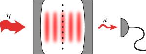
In Ref. Cormick_2012 we analyzed the equilibrium configurations and dynamics of an ion chain close to the linear-zigzag instability Fishman et al. (2008) and confined inside a high-finesse optical resonator. We showed that linear and zigzag arrays are bistable for certain strengths of the laser pumping the cavity. For these regimes we argued that the chain is cooled into one of the configurations by cavity-enhanced photon scattering, exhibiting steady-state entanglement between photonic and vibrational fluctuations. In the present work we characterize the stationary state of the ion chain in detail, focusing on the configuration in Fig. 1. We derive a comprehensive theoretical model which allows us to find the regime in which the chain exhibits bistable structures. The steady state of cavity and vibrational excitations is determined within a semiclassical approximation and the spectrum of light at the cavity output is evaluated. It is shown that motional and field fluctuations are entangled in the parameter regime where bistability is found. The entanglement is studied as a function of the pump strength by means of the logarithmic negativity Vidal and Werner (2002), and its signatures are identified in the spectrum of the light at the cavity output.

This work is organized as follows. In Sec. II the theoretical model of the system is introduced. In Sec. III.1 we describe the semiclassical treatment of the problem, and in Sec. III.2 the equilibrium configurations of the crystal and cavity mode are analyzed as a function of the system parameters. Section III.3 is devoted to the effect of the cavity field on the structural stability. The equations governing the dynamics of the fluctuations of cavity field and motion about their equilibrium values are derived in Sec. III.4, and their solution is discussed in Sec. III.5. In Sec. IV the stationary state of the fluctuations is characterized. The mean excitation number of the different vibrational modes due to cavity cooling is reported in Sec. IV.1, the spectrum of the light at the cavity output is given in Sec. IV.2, and the entanglement between cavity and motional fluctuations is determined in Sec. IV.3. The conclusions are drawn in Sec. V, while the appendices provide details of the calculations relevant to Sec. III.5 and Sec. IV.2.

II Ion chains in a quantum potential

II.1 The model

We consider $N$ ions of mass $m$ and charge $q$ confined by a harmonic potential. We assume for simplicity that the motion of the ions is restricted to the $x-y$ plane, and denote the frequencies of the harmonic trap by $\omega_{x}$ and $\omega_{y}$. In absence of coupling to other physical objects, their dynamics is determined by Hamiltonian

$$H_{\rm ions}=\!\sum_{j=1}^{N}\Bigg{[}\frac{\mathbf{p}_{j}^{2}}{2m}+V_{\rm trap}(\mathbf{r}_{j})+\!\!\!\sum_{k=j+1}^{N}\!\!\!V_{\rm Coul}(|\mathbf{r}_{j}-\mathbf{r}_{k}|)\Bigg{]}\,,$$ (1)

where the operators $\mathbf{r}_{j}$ and $\mathbf{p}_{j}$ denote the position and momentum of the center of mass of the $j$-th ion in the $x-y$ plane. $H_{\rm ions}$ includes the kinetic energy, the trap potential

$$V_{\rm trap}(\mathbf{r}_{j})=\frac{m}{2}(\omega_{x}^{2}x_{j}^{2}+\omega_{y}^{2}y_{j}^{2})\,,$$ (2)

and the Coloumb repulsion

$$V_{\rm Coul}(|\mathbf{r}_{j}-\mathbf{r}_{k}|)=\frac{q^{2}}{4\pi\epsilon_{0}}\frac{1}{\left|\mathbf{r}_{j}-\mathbf{r}_{k}\right|}\,.$$ (3)

At sufficiently low temperatures, which can be achieved by means of Doppler cooling, the ions crystallize at the equilibrium positions determined by the trap potential and by the Coulomb repulsion Dubin_RMP99 . In this regime, if $\omega_{x}$ exceeds a critical value $\omega_{crit}$ (which depends on $\omega_{y}$ and $N$), the ions form a linear array along the $y$ direction Birkl et al. (1992); Birkl_PRL92 ; Dubin_PRL_1993 ; Morigi_2004 . For $\omega_{x}$ below $\omega_{crit}$ but sufficiently close to it, the Coulomb repulsion pushes the ions away from the $y$ axis and the new equilibrium configuration has the geometry of a zigzag Birkl et al. (1992); Birkl_PRL92 ; Dubin_PRL_1993 ; James_PRL_2000 ; Morigi_2004 ; Piacente_PRB_2004 ; Fishman et al. (2008).

In this article we assume that the ion chain is placed inside an optical resonator as shown in Fig. 1, with $\omega_{x}>\omega_{crit}$. A dipolar transition of the ions, formed by the ground state $|{g}\rangle$ and the excited state $|{e}\rangle$ at transition frequency $\omega_{0}$, strongly couples with a cavity mode at frequency $\omega_{c}$, which in turn is pumped by a laser at frequency $\omega_{p}$. The Hamiltonian describing the system dynamics, composed by the cavity mode and the ions’ internal and external degrees of freedom, reads

$$H=H_{\rm cav}+H_{\rm el}+H_{\rm ions}+H_{\rm JC}\,,$$ (4)

where

$$H_{\rm cav}=-\hbar\Delta_{c}a^{\dagger}a-{\rm i}\hbar(\eta^{*}a-\eta a^{\dagger})$$ (5)

is the Hamiltonian for the cavity mode in the reference frame rotating with the laser frequency, with $a$ and $a^{\dagger}$ the annihilation and creation operators of a cavity photon, $\Delta_{c}=\omega_{p}-\omega_{c}$ the detuning between laser and cavity-mode frequency, while the frequency $\eta$ gives the strength of the pumping by the external laser. The term

$$H_{\rm el}=-\hbar\Delta_{0}\sum_{j=1}^{N}|e\rangle_{j}\langle e|$$ (6)

accounts for the internal atomic dynamics, with $\Delta_{0}=\omega_{p}-\omega_{0}$ the detuning of the pump from the dipolar transition. Finally, the dipolar coupling between the cavity and the particles reads

$$H_{\rm JC}=\hbar\sum_{j=1}^{N}g(\mathbf{r}_{j})(\sigma_{j}a^{\dagger}+\sigma^{\dagger}_{j}a)$$ (7)

and describes the absorption of a photon accompanied by the excitation of the atom $j$, given by the raising operator $\sigma^{\dagger}_{j}=|e\rangle_{j}\langle g|$, and the emission with corresponding atomic de-excitation by the lowering operator $\sigma_{j}$. Frequency $g(\mathbf{r}_{j})$ is the coupling strength between the cavity mode and the ion at position ${\bf r}_{j}$. It is modulated by the amplitude of the cavity field at the position of the atom and is here assumed to take the form

$$g(\mathbf{r})=g_{0}\cos(kx)e^{-y^{2}/(2w^{2})}\,,$$ (8)

where $g_{0}$ is the maximum value that the function $|g(\mathbf{r})|$ can take, $k$ is the modulus of the cavity wave vector $\mathbf{k}$ pointing along the $x$ axis, and $w$ is the width of the Gaussian transverse profile of the mode, with $kw\gg 1$.

In addition, the coupling to the modes of the electromagnetic field external to the resonator gives rise to cavity losses at rate 2$\kappa$ (we neglect here photon absorption at the cavity mirrors) and to spontaneous decay of the atomic transition at rate $\gamma$. The incoherent effects are included in the dynamics using Heisenberg-Langevin equations for the operators Gardiner and Collett (1985); Szirmai et al. (2010). For instance, the equations of motion for the operators $a$ and $\sigma_{j}$ read:

$$\dot{a}=\frac{1}{{\rm i}\hbar}[a,H]-\kappa a+\sqrt{2\kappa}\,a_{\rm in}(t)$$ (9)

$$\dot{\sigma_{j}}=\frac{1}{{\rm i}\hbar}[\sigma_{j},H]-\frac{\gamma}{2}\sigma_{j}+\sqrt{\gamma}\,\sigma_{j,\rm in}(t)\,,$$ (10)

with input noise $a_{\rm in}$ and $\sigma_{j,\rm in}(t)$ for field and atom, respectively. Denoting by $\zeta_{\rm in}(t)=a_{\rm in}(t),\,\sigma_{j,\rm in}(t)$, the input noise operators have vanishing expectation value, $\langle\zeta_{\rm in}(t)\rangle=0$, and correlations satisfying the relation

$$\langle[\zeta_{\rm in}(t^{\prime}),\zeta_{\rm in}^{\dagger}(t^{\prime\prime})]\rangle=\delta(t^{\prime}-t^{\prime\prime})\,.$$ (11)

The state of the electromagnetic field outside the cavity is assumed to be thermal with mean number of photons $\bar{n}(\omega_{c})\approx 0$ at frequency $\omega_{c}$, such that

$$\langle\zeta_{\rm in}^{\dagger}(t^{\prime})\zeta_{\rm in}(t^{\prime\prime})\rangle=0\,.$$ (12)

The equations of motion for $a^{\dagger}$ and $\sigma_{j}^{\dagger}$ are the Hermitian conjugate of Eq. (9) and Eq. (10), respectively. The ions’ motion is affected by other sources of noise such as patch potentials in the electrodes. A specific model for the noise on the motion will be introduced in Section III.4.

II.2 The quantum potential

In this paper we characterize structural transitions induced by the coupling of the ion chain with the cavity field. We consider the situation in which the linear chain in free space is stable, namely, $\omega_{x}>\omega_{crit}$, but close to the mechanical instability, and we study the effect of the strong coupling with the cavity field on the structural stability. We focus on the regime in which the detuning of the laser pump with respect to the atom, $\Delta_{0}$, determines the fastest time scale, such that $|\Delta_{0}|\gg\gamma,\kappa,|\Delta_{c}|,g_{0}\sqrt{\bar{n}}$, with $\bar{n}$ the mean intracavity photon number. In this case, the excited state of the atoms can be adiabatically eliminated from the equations of motion for cavity and ions’ external motion, leading to the effective interaction

$$H_{\rm int}=\hbar\,a^{\dagger}a\,U_{0}(\mathbf{r}_{1},\ldots,\mathbf{r}_{N})\,,$$ (13)

where $U_{0}$ reads

$$U_{0}(\mathbf{r}_{1},\ldots,\mathbf{r}_{N})=\sum_{j=1}^{N}\frac{g^{2}(\mathbf{r}_{j})}{\Delta_{0}}\,,$$ (14)

and weighs the nonlinear coupling between motion and cavity mode. Under this condition, the Hamiltonian governing the dynamics of cavity field and external degrees of freedom of the ions now reads $H=H_{\rm ions}+H_{\rm cav}+H_{\rm int}$. Frequency $U_{0}$ is the shift of the cavity frequency due to the ions inside the resonator, and conversely it is the mechanical potential exerted on these ions by a single cavity photon Domokos_Ritsch_2002 ; Maschler and Ritsch (2005); Larson et al. (2008). Hamiltonian $H_{\rm int}$ thus can be interpreted as a quantum potential for the atoms, being its amplitude dependent on the number of intracavity photons. This term gives rise to mechanical effects that, for strong coupling, can be significant even at the single-photon level. Parameter $U_{0}$ also scales photon losses due to spontaneous emission. In fact, for a given set of ions’ positions the cavity decay rate reads $\kappa_{\rm eff}=\kappa+U_{0}\gamma/(2\Delta_{0})$. In the following we shall restrict to the regime in which the cavity-ion interaction is mainly dispersive and spontaneous emission can be thus neglected.

III Stationary state

In this section we determine the stationary state of the coupled system, in the regime in which the relevant degrees of freedom are the external motion of the ions and the cavity field, which are coupled via the effective potential in Eq. (13).

III.1 The semiclassical limit

We perform the study in the semiclassical limit, assuming that the fluctuations about the mean values of field and atomic variables are sufficiently small to justify the treatment. To this aim, we decompose the operators as a sum of mean values and fluctuations according to the prescription

$$\begin{array}[]{l}a=\bar{a}+\delta a\,,\\ \mathbf{r}_{j}=\bar{\mathbf{r}}_{j}+\delta\mathbf{r}_{j}\,,\\ \mathbf{p}_{j}=\bar{\mathbf{p}}_{j}+\delta\mathbf{p}_{j}\,,\end{array}$$ (15)

where $\langle a\rangle=\bar{a}$, $\langle\mathbf{r}_{j}\rangle=\bar{\mathbf{r}}_{j}$, and $\langle\mathbf{p}_{j}\rangle=\bar{\mathbf{p}}_{j}$, while the expectation value of the fluctuations $\delta a,\delta\mathbf{r}_{j},\delta\mathbf{p}_{j}$ vanishes. The mean values satisfy the equations of motion

$$\frac{\partial~{}}{\partial t}\bar{a}=({\rm i}\Delta_{\rm eff}-\kappa)\bar{a}+\eta\,,$$ (16)

$$\frac{\partial~{}}{\partial t}\bar{\mathbf{r}}_{j}=\frac{\bar{\mathbf{p}}_{j}}{m}\,,$$ (17)

$$\frac{\partial~{}}{\partial t}\bar{\mathbf{p}}_{j}=-\nabla_{j}H_{\rm ions}-\hbar|\bar{a}|^{2}\nabla_{j}U_{0}\,,$$ (18)

with $\nabla_{j}$ the gradient with respect to the spatial coordinates of the $j$-th particle (evaluated at the equilibrium positions $\bar{\mathbf{r}}_{1},\ldots,\bar{\mathbf{r}}_{N}$), while

$$\Delta_{\rm eff}=\Delta_{c}-U_{0}(\bar{\mathbf{r}}_{1},\ldots,\bar{\mathbf{r}}_{N})\,.$$ (19)

In order to determine the classical equilibrium values we require that the quantities $\bar{a}$, $\bar{\mathbf{r}}_{j}$ and $\bar{\mathbf{p}}_{j}$ correspond to stationary solutions of the dynamical equations, namely $\partial_{t}\bar{a}=0$, $\partial_{t}\bar{\mathbf{r}}_{j}=0$, and $\partial_{t}\bar{\mathbf{p}}_{j}=0$.

The coupled dynamics of the quantum fluctuations of field and motion are governed by the Heisenberg-Langevin equations Gardiner and Collett (1985); Szirmai et al. (2010), which are found substituting the decomposition (15) into Eq. (9) and into the Heisenberg equations of motion for the center-of-mass variables, and using that the mean values are the stationary solutions. The equations read

$$\delta\dot{a} =({\rm i}\Delta_{\rm eff}-\kappa)\delta a-{\rm i}\bar{a}\sum_{k}(\delta\mathbf{r}_{k}\nabla_{k})U_{0}+\sqrt{2\kappa}\,a_{\rm in}\,,$$ (20)

$$\dot{\delta\mathbf{r}_{j}} =\frac{\delta\mathbf{p}_{j}}{m}\,,\phantom{\sum_{k}}$$ (21)

$$\dot{\delta\mathbf{p}_{j}} =-\sum_{k}(\delta\mathbf{r}_{k}\nabla_{k})\left(\nabla_{j}H_{\rm ions}+\hbar|\bar{a}|^{2}\nabla_{j}U_{0}\right)$$

$$\quad\,-\hbar\left({\bar{a}}^{*}\delta a+\bar{a}\delta a^{\dagger}\right)\nabla_{j}U_{0}\,,$$ (22)

where the derivatives in the expressions above are evaluated at the equilibrium positions. With no loss of generality, we choose the phase of $\eta$ such that $\bar{a}$ is real.

III.2 Equilibrium configurations

We first focus on the equilibrium configuration found by setting Eqs. (16)-(18) equal to zero. From Eq. (16) the equilibrium value of the cavity field amplitude reads

$$\bar{a}=\frac{\eta}{\kappa-{\rm i}\Delta_{\rm eff}}\,,$$ (23)

and depends on the positions of the ions. Setting Eq. (17) to zero gives $\bar{\mathbf{p}}_{j}=0$, and finally from Eq. (18) one finds that the equilibrium positions of the ions must be minima of an effective potential of the form

$$V_{\rm tot}=V_{\rm trap}+V_{\rm Coul}+V_{\rm eff}\,,$$ (24)

where the term

$$V_{\rm eff}=\frac{\hbar|\eta|^{2}}{\kappa}\arctan\left(-\frac{\Delta_{\rm eff}}{\kappa}\right)$$ (25)

is due to the coupling with the cavity field. The back-action of the cavity field on the ions, in particular, enters in Eq. (25) via the parameter $\Delta_{\rm eff}$, Eq. (19), and scales with $U_{0}$. Whether cavity back-action is relevant to the dynamics can be determined by means of the dimensionless parameter

$$\mathcal{C}=\frac{g_{0}^{2}N_{\rm eff}}{\kappa|\Delta_{0}|}\,,$$ (26)

where $N_{\rm eff}$ is the effective number of ions that couple to the field mode, defined as:

$$N_{\rm eff}=\sum_{j=1}^{N}e^{-\bar{y}_{j}^{2}/w^{2}}.$$ (27)

Parameter (26) can be identified with the cooperativity Kimble . For $\mathcal{C}\gtrsim 1$ the potential in Eq. (25) gives rise to an effective long-range force between the ions. On the other hand, in the limit $\mathcal{C}\ll 1$ the effect of the ions on the field is negligible. Then, the mean value of the cavity field is determined by external parameters, so that $\bar{a}=\eta/(\kappa-i\Delta_{c})$ and Eq. (13) is well approximated by a classical potential of the form:

$$V_{\rm opt}=\frac{\hbar\,|\eta|^{2}}{\kappa^{2}+\Delta_{c}^{2}}\,\sum_{j=1}^{N}\frac{g^{2}(\mathbf{r}_{j})}{\Delta_{0}}\,,$$ (28)

which overlaps to the trap and Coulomb potential.

In this paper we analyze the case when the string is orthogonal to the cavity-mode wave vector, as in Fig. 1, corresponding to the limit $\omega_{x}\gg\omega_{y}$. The formalism developed so far, however, is valid for any structure that the ions can take. It can be applied, hence, also for the specific case in which the ions form a string which is parallel to the cavity axis. In our model, this case corresponds to setting $\omega_{y}\gg\omega_{x}$ so that the equilibrium configuration has values $y_{j}=0$ for $j=1,,\ldots,N$. For small cooperativity, $\mathcal{C}\ll 1$, the equilibrium positions along $x$ correspond to minima of the total potential:

$$V_{\rm FKM}=\sum_{j=1}^{N}\Bigg{[}\frac{m}{2}\omega_{x}^{2}x_{j}^{2}+\sum_{k=j+1}^{N}\frac{q^{2}}{4\pi\epsilon_{0}}\frac{1}{\left|x_{j}-x_{k}\right|}\\ +\frac{\hbar\,|\eta|^{2}}{\kappa^{2}+\Delta_{c}^{2}}\frac{g_{0}^{2}}{\Delta_{0}}\,\cos^{2}(kx_{j})\Bigg{]}\,,$$ (29)

and can be mapped to a Frenkel-Kontorova model García-Mata et al. (2007); Pruttivarasin et al. (2011). Upon varying the depth of the optical potential, this model exhibits a classical transition between sliding and pinned phases, which has been proposed to study friction Benassi et al. (2011), and a quantum transition between a pinned instanton glass and a sliding phonon gas García-Mata et al. (2007). If, instead, the effective cooperativity $\mathcal{C}$ is larger than unity, the term associated to the optical potential introduces also an additional, infinitely-ranged interaction between the particles, giving rise to dynamics which are largely unexplored to date.

III.3 Multistability

We shall assume that the string is orthogonal to the cavity-mode wave vector, as in Fig. 1. Such a scenario can be realized, for instance, with the setups of Refs. Keller et al. (2004); Stute et al. (2012). In this case the optical potential generates a transverse force, which is symmetric about the chain axis when the chain is at a node or antinode of the cavity standing wave.

We first consider small cooperativities, $\mathcal{C}\ll 1$. If all ions are illuminated by the cavity mode, close to the linear-zigzag mechanical instability the optical potential shifts the critical value of the transverse trap frequency $\omega_{x}$ with respect to the free-space value $\omega_{crit}$. If only a part of the chain is illuminated, at a value $\omega_{x}>\omega_{crit}$ a local structural distortion will appear with the form of a zigzag chain. Let us assume that the equilibrium positions of the ions in the linear array are located at an antinode of the cavity mode. For blue-detuned pumps, with $\Delta_{0}>0$, the light field pushes the particles away from the antinode and a mechanical instability thus appears at frequencies $\omega_{x}$ larger than $\omega_{crit}$, while a red-detuned pump field has the opposite effect. We note that these generic considerations, which are valid for the secular potential of a Paul trap, can also be applied when the micromotion is taken into account. In fact, the plane containing the zigzag array can be chosen to be such that micromotion is in the direction perpendicular to the plane and therefore has no effect on the problem under study.

III.3.1 Multistable structures

The dynamical behaviour of the system is significantly modified at large cooperativities, $\mathcal{C}\gtrsim 1$, where the cavity-mediated interaction between the ions becomes relevant. This property introduces an additional nonlinearity. For definiteness, from now on we take $\Delta_{c}=0$, $\Delta_{0}>0$, and we restrict to the case when $\omega_{x}>\omega_{crit}$ so that in the absence of pumping the particles form a linear array along $x=0$, coinciding with an antinode of the cavity field. Therefore, the effective detuning $|\Delta_{\rm eff}|$ is maximum when the chain is in the linear configuration. For a fixed pumping strength $\eta\neq 0$, the intracavity field intensity increases if the equilibrium positions are shifted to a zigzag. This optical nonlinearity can lead to bistable linear and zigzag configurations, in contrast to the continuous linear-zigzag transition in free space. This can be better understood by analyzing the effective potential $V_{s}$ of the zigzag mode. We start from the knowledge that the zigzag mode is the soft mode of the linear-zigzag transition in free space and that an effective, Landau potential for the soft mode can be derived, whose equilibrium solutions are either the linear or the zigzag configurations Fishman et al. (2008). We then study how the effective potential is modified by the coupling with the cavity, thereby discarding the coupling with the other vibrational modes that may arise due to the cavity field. We first consider the simplest limit assuming that the ions of the linear array are equidistant. In this case the zigzag mode amplitude reads $x_{s}=\sum_{j}(-1)^{j}x_{j}/\sqrt{N}$, while the zigzag amplitude, equal to twice the transverse equilibrium displacement of the ions from the $x=0$ axis, is $b=2x_{s}/\sqrt{N}$. Denoting by $\omega_{s}=\sqrt{\omega_{x}^{2}-\omega_{crit}^{2}}$ the frequency of the soft mode in free space and above the critical point, the potential $V_{s}$ can be written as

$$V_{s}=\frac{m\omega_{x}^{2}}{k^{2}}\left\{\frac{\vartheta}{2}\left(\frac{kb}{2}\right)^{2}+2P\arctan\left[\mathcal{C}\cos^{2}\left(\frac{kb}{2}\right)\right]\right\}\,,$$ (30)

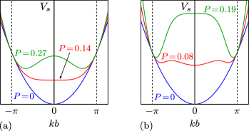
where we assumed that the ions are uniformly illuminated by the cavity field. The first term on the right-hand side of Eq. (30) describes the harmonic potential for the soft mode in free space, with $\vartheta=N\omega_{s}^{2}/\omega_{x}^{2}$. The second term corresponds to the optical potential, proportional to the dimensionless power $P=|\eta|^{2}\omega_{R}/(\kappa\omega_{x}^{2})$, with $\omega_{R}=\hbar k^{2}/(2m)$ the recoil frequency. The form of the potential $V_{s}$ is shown in Fig. 2 for different values of $\mathcal{C}$ and $P$. The stability of the linear configuration is determined by $\mathcal{C}$ and by the ratio $P/\vartheta$ and corresponds to the presence of a minimum at $b=0$. For $P=0$ the cavity mode is in the vacuum state and the linear array is stable. The soft mode becomes unstable when the optical power is increased above the threshold value $P=\vartheta(1+\mathcal{C}^{2})/(4\mathcal{C})$. For large cooperativities, there are parameter regimes for which both linear and zigzag configurations are stable, as illustrated by the appearance of three minima in Fig. 2(b) for intermediate values of the pump power.

Figure 2: (color online) Potential $V_{s}$ of the zigzag mode, Eq. (30), as a function of the zigzag amplitude $b$ (in units of $1/k$) for different pumping powers $P$ (in units of $P_{0}=\kappa\omega_{x}^{2}/\omega_{R}$). The dashed lines indicate the nodes of the cavity mode at $kb=\pm\pi$. The cooperativity is (a) $\mathcal{C}=0.5$ and (b) $\mathcal{C}=3$. The coupling of the ions with the field is assumed to be homogeneous and $\vartheta=N\omega_{s}^{2}/\omega_{x}^{2}=0.22$.

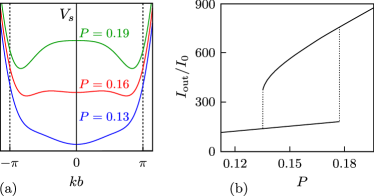
These results are based on the assumption that the interparticle distance is uniform. Such model can be realized in a ring trap Birkl et al. (1992) or in a multipolar radiofrequency trap Okada et al. (2007); Champenois et al. (2010), and it approximates a chain in an axial anharmonic trap Lin et al. (2009). For a chain in a linear Paul trap, however, the interparticle distance varies Dubin:1997 , and neither the coupling of the ions to the cavity nor the corresponding amplitude of the soft mode are uniform along the chain DeChiara_NJP:2010 . Figure 3(a) displays $V_{s}$ for a chain of 60 ions in a harmonic trap, where the central region of the chain couples to the cavity mode with $N_{\rm eff}\sim 5.7$. Here, for certain values of the pumping strength the potential $V_{s}$ also exhibits three minima, corresponding to stable linear and zigzag arrays. We note that close to the instability the equilibrium positions in the zigzag configuration are very similar in geometry to the soft mode of the linear chain.

III.3.2 Intensity of the light at the cavity output

The bistable behaviour can be detected by monitoring the mean value of the intensity $I_{\rm out}$ of the field at the cavity output. This is found from the mean value of the field at the cavity output, $a_{\rm out}=\sqrt{2\kappa}a+a_{\rm in}$ and reads

$$I_{\rm out}=2\kappa|\bar{a}|^{2}\,.$$ (31)

Figure 3(b) displays $I_{\rm out}$ as a function of the pump intensity. The lower branch corresponds to the light at the cavity output when the ions form a linear array, and the upper branch to a zigzag array. The presence of two different values of the output intensity for a given pump power indicates bistable equilibrium configurations of the ions’ structure.

Figure 3: (color online) (a) Same as Fig. 2 but for a chain in a linear Paul trap. A chain of 60 ⁴⁰Ca⁺ ions is taken with interparticle distance 4.3 $\mu$m in the central region. The ions are coupled to a cavity mode with wavelength 866 nm and transverse width $w=14\,\mu$m ($N_{\rm eff}\simeq 5.7$). (b) Intensity $I_{\rm out}$ at the cavity output as a function of $P$. Here, the intensity is in units of $I_{0}=I_{\rm out}(P_{0})$, and for a configuration minimizing $V_{\rm tot}$, numerically found using linear and zigzag chains as initial guesses. The other parameters are $\omega_{y}=2\pi~{}\times$ 0.1 MHz, $\omega_{x}=2\pi~{}\times$ 2.26 MHz (the critical value is $\omega_{crit}\simeq 2\pi~{}\times$ 2.216 MHz), $\Delta_{c}=0$, $\Delta_{0}=2\pi~{}\times$ 500 MHz, $\kappa=2\pi~{}\times$ 0.5 MHz, $g_{0}=2\pi~{}\times$ 9.4 MHz, $\gamma=2\pi~{}\times$ 10 MHz, resulting in $\mathcal{C}=2$.

III.3.3 Discussion

The bistability we predict is a consequence of the dependence of the optical potential on the positions of the atoms within the standing-wave field. In the thermodynamic limit, if the region of the chain interacting with the cavity mode is finite, the effect of this coupling is a localized defect in the chain. For a finite system, nevertheless, forces acting on few ions can generate arrays close to zigzag configurations due to the long-range Coulomb repulsion Baltrusch et al. (2011); Li and Lesanovsky (2012).

The observed bistable behaviour shares several analogous features with textbook optical bistability Lugiato . The nonlinear dynamics here studied, however, are solely due to the interplay between the dispersive optomechanical coupling of the ions’ external motion with the cavity field and the long-range Coulomb interaction, for configurations in which the net force over the ions vanishes. The nonlinear dependence on the ion positions enters via the Coulomb repulsion and the detuning $\Delta_{\rm eff}$, Eq. (19), in the cavity-induced term of the total potential in Eq. (24). Therefore, bistability in this case is not necessarily found for the configurations where the mean amplitude of the field in Eq. (23) exhibits local maxima, which would correspond to configurations where $\Delta_{\rm eff}$ vanishes. This is a major difference with bistability effects in the optomechanical coupling between neutral atoms and cavity fields Hemmerich ; StamperKurn ; Ritter ; Larson:2009 , where the strong coupling with the cavity gives rise to the most relevant nonlinearity. We note that optomechanical bistability, for media constituted by neutral quantum gases, can be associated with different quantum phases of ultracold atomic gases of bosons Larson et al. (2008); Meystre . Analogously, in our case bistability is associated with different classical structures.

III.4 Quantum fluctuations

We now analyze the dynamics of the fluctuations of the system observables about the equilibrium values close to the linear-zigzag instability, where multistability due to the strong coupling with the cavity mode is observed. We restrict to the case when these fluctuations are sufficiently small that the system admits a linearized description. This requires the validity of the Lamb-Dicke approximation Stenholm_1986 , namely, the displacements from the equilibrium positions have to be smaller than the light wavelength (therefore, this treatment is not valid in the very close vicinity of the structural transition or at high temperatures).

For convenience we introduce the normal modes of the crystal, that characterize the dynamics of the ions when the coupling with the quantum fluctuations of the cavity field can be neglected. We hence write the displacements of the ions as:

$$\delta x_{j}=\sum_{n}M_{jn}^{(x)}q_{n}\,,\quad\delta y_{j}=\sum_{n}M_{jn}^{(y)}q_{n},\\$$ (32)

with $M_{jn}^{(x,y)}$ the element of the orthogonal matrix relating the local coordinates $\delta x_{j}$, $\delta y_{j}$ with the normal-mode coordinates $q_{n}$. The normal-mode coordinates diagonalize Eqs. (21)-(III.1) when the cavity fluctuations $\delta a$ are set to zero. We note that this is not equivalent to setting the cavity field to zero, since we define the normal modes taking into account the optical potential determined by the mean value of the field.

We denote by $b_{n}$ and $b_{n}^{\dagger}$ the bosonic operators annihilating and creating, respectively, an energy quantum (phonon) of the normal mode at frequency $\omega_{n}$. They are defined through the equations $q_{n}=\sqrt{\hbar/(m\omega_{n})}Q_{n}$ and $p_{n}=\sqrt{\hbar m\omega_{n}}P_{n}$, with

$$Q_{n}=\frac{b_{n}+b_{n}^{\dagger}}{\sqrt{2}},\quad~{}P_{n}={\rm i}\frac{b_{n}^{\dagger}-b_{n}}{\sqrt{2}}\,.$$ (33)

The dynamical equations for motional modes and photonic fluctuations take then the form:

$$\delta\dot{a}=({\rm i}\Delta_{\rm eff}-\kappa)\delta a-{\rm i}\bar{a}\sum_{n}c_{n}(b_{n}+b_{n}^{\dagger})+\sqrt{2\kappa}\,a_{\rm in}\,,$$ (34)

$$\dot{b}_{n}=-({\rm i}\omega_{n}+\Gamma_{n})b_{n}-{\rm i}\bar{a}c_{n}(\delta a+\delta a^{\dagger})+\sqrt{2\Gamma_{n}}\,b_{{\rm in},n}\,,$$ (35)

which also includes the effect of a noise source heating the vibrational mode $n$ at rate $\Gamma_{n}$. The corresponding Langevin force is described by the input noise operator $b_{{\rm in},n}$, with $\langle b_{{\rm in},n}\rangle=0$ and Gardiner and Collett (1985):

$$\langle b_{{\rm in},n}^{\dagger}(t^{\prime})\,b_{{\rm in},n^{\prime}}(t^{\prime\prime})\rangle=\bar{N}_{n}\,\delta_{nn^{\prime}}\,\delta(t^{\prime}-t^{\prime\prime})\,.$$ (36)

Here, $\bar{N}_{n}=\bar{N}(\omega_{n})$ is the mean excitation number of an oscillator of frequency $\omega_{n}$ at the temperature of the considered environment . These terms introduce a simple model simulating the heating observed in an ion trap Häffner et al. (2008); Wineland et al. (1998); James_PRL98 ; Henkel_1999 .

The coefficients $c_{n}$ in Eq. (34)-(35) give the coupling strength between motional and cavity field fluctuations. They read

$$c_{n}=\sqrt{\frac{\hbar}{2m\omega_{n}}}\sum_{j}\left[M_{jn}^{(x)}\partial_{x_{j}}+M_{jn}^{(y)}\partial_{y_{j}}\right]U_{0}\,,$$ (37)

where the derivatives are evaluated at the equilibrium positions $\bar{\mathbf{r}}_{j}$. They vanish when the equilibrium positions $\bar{\mathbf{r}}_{j}$ are located at field nodes. If the particles are instead at antinodes, the coupling is determined by the derivatives in $y$ direction, which are assumed to be much smaller than those along $x$ (since $kw\gg 1$). As we assume that when the ions form a linear chain they lie at an antinode, the coupling between vibrations and field fluctuations is much stronger in the zigzag configuration than for the linear array.

III.5 Solution of the linearized coupled evolution of fluctuations

We now solve the linear inhomogeneous system of differential equations (34)-(35). Following a standard procedure, we look for the solution of the homogeneous system and for a particular solution of the inhomogeneous equations Vitali_2008 ; Tufarelli et al. (2012). We first introduce dimensionless quadrature operators for field and ions’ motion,

$$X_{a}=\begin{pmatrix}Q_{a}\\ P_{a}\end{pmatrix}\,,\quad X_{n}=\begin{pmatrix}Q_{n}\\ P_{n}\end{pmatrix}\,,$$ (38)

with the field quadratures

$$Q_{a}=\frac{\delta a+\delta a^{\dagger}}{\sqrt{2}},\quad P_{a}=-{\rm i}\>\frac{\delta a-\delta a^{\dagger}}{\sqrt{2}}\ ,$$ (39)

while $Q_{n}$ and $P_{n}$ are defined in Eq. (33). We then arrange them together in a column vector,

$$\vec{X}=\begin{pmatrix}X_{a}\\ X_{1}\\ X_{2}\\ \vdots\\ X_{N}\end{pmatrix}\,,$$ (40)

and rewrite Eqs. (34)-(35) in the compact form

$$\frac{d\vec{X}}{dt}=M\vec{X}+\vec{X}_{\rm in}(t)\,.$$ (41)

Here, $\vec{X}_{\rm in}$ contains the input noise operators, while

$$M=\begin{pmatrix}M_{a}&A_{1}&A_{2}&\ldots&A_{N}\\ A_{1}&M_{1}&0&\ldots&0\\ A_{2}&0&M_{2}&\dots&0\\ \vdots&\vdots&\vdots&\ddots&\vdots\\ A_{N}&0&0&\ldots&M_{N}\end{pmatrix}\,,$$ (42)

where

$$M_{a}=-\kappa\,\mathbb{I}-{\rm i}\,\Delta_{\rm eff}\,\sigma_{y}\,,$$ (43)

$$M_{n}=-\Gamma_{n}\,\mathbb{I}+{\rm i}\,\omega_{n}\,\sigma_{y}\,,$$ (44)

$$A_{n}=-\bar{a}\,c_{n}(\sigma_{x}-{\rm i}\,\sigma_{y})\,,$$ (45)

and $\sigma_{x,y,z}$ the Pauli matrices.

For each specific set of coefficients, the solution can be found by diagonalizing $M$. The time evolution of the eigenvector of $M$ with eigenvalue $\lambda$ will follow an exponential function, which is decreasing (increasing) if the real part $\Re(\lambda)$ is negative (positive), and oscillating if $\lambda$ is purely imaginary. Therefore, the stability of the system requires that there are no eigenvalues with positive real parts . For a stable system, the values of $-\Re(\lambda)$ determine the rates with which excitations decay. In particular, if the cavity is the only environment the trace of $M$ is $-2\kappa$, which equals the sum of all the eigenvalues of the system. This shows that the total cooling rate due to the coupling with the cavity cannot exceed $2\kappa$, so that the cooling of a higher number of modes can only come at the price of lower cooling rates for each mode.

The eigenvalues $\lambda$ of $M$ satisfy the equation

$$\Delta_{\rm eff}^{2}+(\kappa+\lambda)^{2}=-4\Delta\bar{a}^{2}\sum_{n}\frac{c_{n}^{2}\omega_{n}}{\omega_{n}^{2}+(\lambda+\Gamma_{n})^{2}}\,,$$ (46)

whose derivation is given in Appendix A. The solutions are found numerically, but some of their properties can be inferred from the form of the equations like, for instance, that complex eigenvalues come always in complex-conjugated pairs. In Appendix A it is also shown that, if $\Delta_{\rm eff}<0$ (the case where multistable configurations are found in Sec. III.3), the condition of stability corresponds to the inequality

$$\Delta_{\rm eff}^{2}+\kappa^{2}\geq-4\Delta_{\rm eff}\,\bar{a}^{2}\sum_{n}\frac{c_{n}^{2}\omega_{n}}{\omega_{n}^{2}+\Gamma_{n}^{2}}\,,$$ (47)

which has been found assuming that the equilibrium positions $\bar{\mathbf{r}}_{j}$ correspond to minima of the effective potential as determined by Eqs. (24)-(25), so $\omega_{n}>0$ for all normal modes of the crystal.

For the cases we analyze in this paper the system of equations is diagonalizable, so that $M=TDT^{-1}$ with $T$ a non-singular matrix and $D$ the diagonal matrix containing the eigenvalues. The solution of Eq. (41) takes the form

$$\vec{X}(t)=Te^{D(t-t_{0})}T^{-1}\vec{X}(t_{0})+\int_{t_{0}}^{t}dt^{\prime}\,Te^{D(t-t^{\prime})}T^{-1}\vec{X}_{\rm in}(t^{\prime})\,,$$ (48)

and will be used in order to evaluate the stationary state of the system.

IV Cooling and stationary entanglement

Figure 4: (color online) Equilibrium configurations in a chain of 4 ions as a function of the pump power $P$. The plots display the value of the $x$ coordinate (in units of $1/k$) of each of the ions as a function of $P$ (in units of $P_{0}=\kappa\omega_{x}^{2}/\omega_{R}$). The cooperativity is $\mathcal{C}=0.3$ (left panels) and $\mathcal{C}=3$ (right panels). The vertical dotted lines in the right panels indicate the limits of the bistability region. In (a) and (b) the chain is centered with respect to the cavity axis, while in (c) and (d) it is displaced by 1.1 $\mu$m in $y$ direction with respect to the cavity center. The arrow in (b) indicates the value of $P$ for the eigenmodes shown in Fig. 5. The ions are labelled from $A$ to $D$, with $A$ and $D$ corresponding to the chain edges. The other parameters are $\Delta_{c}=0$, $\Delta_{0}=2\pi~{}\times$ 500 MHz, $\kappa=2\pi~{}\times$ 0.5 MHz, $\gamma=2\pi~{}\times$ 10 MHz, $\omega_{y}=\kappa=2\pi~{}\times$ 1 MHz, $\omega_{x}=2\pi~{}\times$ 2.12 MHz (the critical value is $\omega_{crit}=2\pi~{}\times$ 2.04 MHz). The width $w$ of the Gaussian mode is equal to the distance between the central ions, which is 4.1 $\mu$m in the linear array.

Figure 5: Schematic representation of the motional modes (ordered by increasing frequency) for the parameters of Fig. 4(b) with $P=0.074~{}P_{0}$ and in the zigzag configuration ($U_{0}$ is 1/5 of its value for the linear chain). The positions are not to scale. The modes that couple to the cavity mode are indicated by a double circle.

The tools developed so far are now employed to characterize the steady state of the ion chain coupled with the cavity mode. We consider the parameter regime for which multistable solutions are found, corresponding to the choice of detunings identified in Sec. III.3, namely, $\Delta_{c}=0$, $\Delta_{0}\gg\gamma$, so that $\Delta_{\rm eff}<0$. In this regime, photon scattering cools the normal modes coupled to the resonator field, thus providing an instance of cavity cooling Vuletić and Chu (2000). As we will show, the strong coupling between field and motional fluctuations leads to distinct signals at the cavity output. A peculiar feature of the stationary state is the entanglement between light and crystalline vibrations, which is found for large enough cooperativity and close to the structural instability.

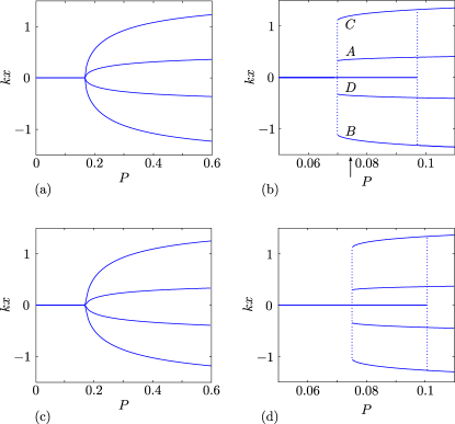
The analytical results presented in this Section are valid for a chain of an arbitrary number $N$ of ions. In order to facilitate the interpretation of the results, the plots will be evaluated for a chain of $N=4$ ions. Figure 4 displays the equilibrium positions along the $x$ axis for different values of the cooperativity and as a function of the pump power $P$. In the right panels one clearly observes bistable regions when the cooperativity is sufficiently large.

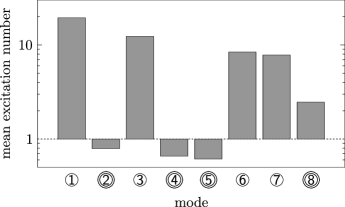
In the following, cooling and entanglement are discussed for two exemplary configurations: in the first configuration, which we will denote by “symmetric configuration”, the chain is centered with respect to the cavity axis. The corresponding equilibrium positions as a function of $P$ are displayed in the upper plots of Fig. 4. In this case, due to the symmetry under reflection about the center of the chain, some vibrational modes are decoupled from the cavity mode. These are, for the zigzag chain, the modes labeled by 1, 3, 6, 7 in Fig. 5. In the second case, which we denote by “asymmetric configuration”, the chain is slightly displaced in $y$ direction. The equilibrium positions of this configuration as a function of $P$ are shown in the lower plots of Fig. 4. In this second case the symmetry is broken and all motional modes can couple to (and thus be cooled by) the cavity field.

IV.1 Stationary state of the fluctuations

We now study the stationary state of the system composed by the cavity fluctuations and the ions’ vibrations about their classical equilibrium values. In general, the knowledge of the density matrix is required. If the initial state is assumed to be Gaussian, it is Gaussian at all times for the noise and dynamics we consider and is hence fully characterized by the first and second moments of the observables $Q_{a},P_{a}$ and $Q_{n},P_{n}$ composing the vector $\vec{X}$ of Eq. (40). For input operators and an initial state with zero mean value, the state is completely described by the covariance matrix A. Ferraro and Paris (2005), whose elements in this case read $C_{\alpha\beta}=\langle X_{\alpha}X_{\beta}+X_{\beta}X_{\alpha}\rangle$, where $\alpha,\beta$ run over all the components of vector $\vec{X}$. The covariance matrix at steady state can be computed using Eq. (48) in the limit $t\to\infty$.

With these results at hand it is straightforward to evaluate the total kinetic energy, mean mode populations, and squeezing. Figure 6 displays the stationary mean occupation number $\langle b^{\dagger}_{n}b_{n}\rangle$ of the $n$-th motional mode for a zigzag chain in the symmetric configuration for parameters for which a bistable configuration is found in Fig. 4(b). Here, it is assumed that the initial state is thermal with temperature $T=1$ mK. The modes which are cooled by photon scattering are the ones in Fig. 5 labeled by 2, 4, 5, 8. At steady state most of them are significantly colder than the uncoupled ones, with mean excitation number smaller than unity. We note that the mode with the highest frequency is colder than the initial temperature but still at a significantly higher temperature than the other modes coupling with the cavity fluctuations. Indeed, this mode corresponds mostly to motion in the $y$ direction, thus weakly coupled to the cavity field.

Figure 6: Mean excitation number $\langle b^{\dagger}_{n}b_{n}\rangle$ for each of the motional modes in Fig. 5. The dotted line indicates the value $\langle b^{\dagger}_{n}b_{n}\rangle=1$ (the vertical axis is in logarithmic scale).

IV.2 Spectrum of light at the cavity output

Information about the dynamical properties of the system in the stationary state can be extracted from the spectrum of the field at the cavity output. Such measurement has been performed, for instance, in Ref. Brahms . Here, we determine the spectrum of the field scattered by the ions at the steady state of the cavity cooling dynamics. We denote by $S(\nu)\propto\langle\tilde{a}_{\rm out}(\nu)^{\dagger}\tilde{a}_{\rm out}(\nu)\rangle$ the component of the spectrum at frequency $\nu=\omega-\omega_{p}$, with $\tilde{a}_{\rm out}$ the Fourier transform of the field at the cavity output, $a_{\rm out}=a_{\rm in}+\sqrt{2\kappa}\,a$. Using that $a=\bar{a}+\delta a$, the quantum component of the spectrum reads

$$S(\nu)=\frac{\langle\delta\tilde{a}(\nu)^{\dagger}\delta\tilde{a}(\nu)\rangle}{\bar{a}^{2}}\,,$$ (49)

where $\delta\tilde{a}(\nu)$ is the Fourier transform of $\delta a$, $\delta\tilde{a}(\nu)^{\dagger}$ is the Hermitian conjugate of $\delta\tilde{a}(\nu)$, and we omit the Rayleigh peak at $\nu=0$, i.e., $\omega=\omega_{p}$, which corresponds to the classical part Bienert et al. (2004). For the setup we consider, when the ions form a linear string they are at an antinode of the cavity field and the coupling of the vibrational modes to the cavity is negligible in the Lamb-Dicke regime (see Sec. III.4). Therefore, for the linear chain the steady-state spectrum exhibits only the Rayleigh peak. When the chain forms a zigzag, the spectrum of the field at the cavity output reads

$$S(\nu)=S_{0}(\nu)\Bigg{\{}\frac{4\kappa\,|\theta(\nu)|^{2}\,\bar{a}^{2}}{\kappa^{2}+(\nu-\Delta_{\rm eff})^{2}}\\ +\sum_{n}c_{n}^{2}\Gamma_{n}\left[\frac{N_{n}}{\Gamma_{n}^{2}+(\omega_{n}-\nu)^{2}}+\frac{N_{n}+1}{\Gamma_{n}^{2}+(\omega_{n}+\nu)^{2}}\right]\Bigg{\}}\,,$$ (50)

and shows the appearance of Fourier components at the frequency of the vibrational modes coupling with the cavity. Expression (50) has been derived by formally integrating Eq. (35) for the evolution of $b_{n}(t)$, replacing in the evolution of the field fluctuations given by Eq. (34), and solving the corresponding system in Fourier space. An alternative form is provided in Appendix B. We now discuss the individual terms on the right-hand side of Eq. (50). The first term inside the curly brackets is the contribution due to the coupling of the quantum vacuum with the cavity field fluctuations, where

$$\theta(\nu)=\sum_{n}\frac{c_{n}^{2}\,\omega_{n}}{\omega_{n}^{2}+(\gamma_{n}-i\nu)^{2}}\,$$ (51)

is a consequence of the coupling with the vibrational modes. The other terms inside the curly brackets are due to the thermal noise on the vibrational modes, and their contribution scales with the corresponding strength of the coupling with the cavity-field fluctuations. The common prefactor reads

$$S_{0}(\nu)=\frac{2}{\kappa^{2}+(\nu+\Delta_{\rm eff})^{2}}\left|1+\frac{4\theta(\nu)\,\Delta_{\rm eff}\,\bar{a}^{2}}{(\kappa-i\nu)^{2}+\Delta_{\rm eff}^{2}}\right|^{-2}\,.$$ (52)

This function becomes a Lorentz curve when ${\mathcal{C}}\ll 1$. This functional behaviour is strongly modified when the cooperativity is increased: Then, motional and quantum noise do not simply add up, but nonlinearly mix to determine the spectral properties of the output field. Figures 7(a) and (b) display the spectra for a chain of four ions in the symmetric configuration, and for two different values of the cooperativity. Note that the Rayleigh peak is not shown. The spectral lines observed in Fig. 7(a) correspond to the sidebands of the normal modes which couple to the cavity field fluctuations. As $\mathcal{C}$ is increased, Fig. 7(b), the spectral lines change the relative heights, width, and shape. We note the asymmetry in the spectra with respect to $\nu=0$: This is due to the (weak) coupling of the ions’ motion to the thermal bath. The broadening at large cooperativity is a consequence of the vacuum input noise and indicates the rate at which the cavity cools the corresponding vibrational mode Bienert et al. (2004). It is accompanied by the appearance of Fano-like resonances which result from the dispersive effect of the cavity back-action and are a signature of quantum interference in the fluctuations of motion and field Fano (1961). This interference is due to quantum correlations established by the dynamics described in Eqs. (34)-(35), and is reminescent of dynamics studied in optomechanical systems Pirandola et al. (2003). For comparison, Figs. 7(c) and (d) show the spectrum for the case in the asymmetric configuration: There, all vibrational modes couple with the cavity field and peaks corresponding to each of the eight motional modes can be identified.

Figure 7: (color online) Spectrum $S(\nu)$ of the field at the cavity output at steady-state for a zigzag of four ions (the Rayleigh peak is not shown). $S(\nu)$ is evaluated from Eq. (50) and reported in units of $\omega_{y}^{-1}$, while $\nu$ is in units of $\omega_{y}$. The upper (lower) panels refer to the symmetric (asymmetric) configuration, where in the asymmetric case the chain is displaced with respect to the cavity axis by 0.28 times the distance between the central ions. The parameters are the same as in Fig. 4 except for (a) $\mathcal{C}=0.3$ and $P=0.54$; (b) $\mathcal{C}=3$ and $P=0.074$; (c) $\mathcal{C}=0.3$ and $P=0.62$; (d) $\mathcal{C}=3$ and $P=0.084$ (the values of $P$ are such that $U_{0}$ is 1/5 of the value it takes when the ions form a linear array). The motion is assumed to couple to a thermal bath at temperature 1mK and thermalization rate $\Gamma_{n}=100$ s^-1 for all modes.

IV.3 Entanglement

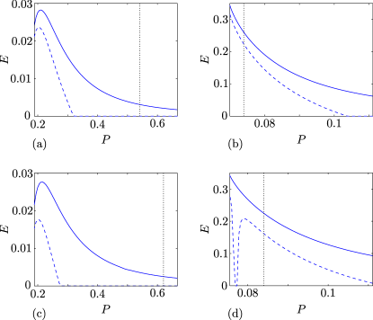
The optomechanical coupling between a cavity mode and an ultracold atomic ensemble has been demonstrated to give rise to non-classical light Brooks . We now show that in our system this coupling generates stationary entanglement between the field fluctuations and the vibrations of the ions about their equilibrium positions. We analyze the presence of entanglement in the system across bipartitions, as quantified by the logarithmic negativity Vidal and Werner (2002). Figure 8 displays the logarithmic negativity for the zigzag chain of four ions as a function of the pumping power. The plots show the entanglement of the cavity field with the whole set of motional modes and with the zigzag mode only, and correspond to the cases in Fig. 4 for pumping powers $P$ at which the zigzag chain is a stable configuration. One clearly observes that quantum correlations between field and vibrations are particularly important for large cooperativity and close to the mechanical instability of the zigzag chain. Besides, correlations are mostly built between the cavity and the zigzag mode, as one can also infer from the broadening of the corresponding spectral peak in Figs. 7(b) and (d), indicating the strong coupling with the cavity field. The results for the asymmetric setup are qualitatively similar to the symmetric case, except that the entanglement between cavity and zigzag mode is smaller. In particular, in Fig. 8(d) one observes that it vanishes for a value of the power that corresponds to an avoided level crossing between two vibrational modes. The plots on the right pannels correspond to an effective cooperativity which is ten times as large as in the left pannels.

A systematic comparison of how entanglement scales with the cooperativity requires to set some criteria. A naive comparison between the values of entanglement as the cooperativity is increased shows that -for the powers $P$ shown in Fig. 8- entanglement is approximatively an order of magnitude larger when the effective cooperativity is increased by the same amount. However, such comparison has some drawbacks. For instance, the transverse equilibrium positions of the ions are different, and for large cooperativity there are no solutions corresponding to zigzags with arbitrarily small amplitude. In addition, our treatment becomes invalid when the Lamb-Dicke approximation does not apply. A possible comparison is then to consider the entanglement between light and vibrations when the ions are at the same equilibrium positions but for different cooperativities. An example is given by the vertical dotted lines in the left and right plots of Fig. 8, which indicate the values of $P$ at which the same equilibrium structures are found at different values of the cooperativity. In this case, we again verify that entanglement increases with the cooperativity. In particular, for the same transverse equilibrium displacements, increasing the cooperativity by a factor of ten can increase the logarithmic negativity by almost two orders of magnitude.

Figure 8: (color online) Entanglement between field and motional fluctuations as a function of pumping power $P$. The entanglement is given by the logarithmic negativity. The continuous line shows the entanglement between the cavity fluctuations and the whole set of vibrational modes, the dashed line the entanglement between the cavity and the zigzag mode only. The parameters are the same as in Fig. 4 for (a)-(d), respectively, but the results here refer only to zigzag configurations and within the Lamb-Dicke regime. The dotted vertical lines indicate the values for which the spectra in Fig. 7 are evaluated.

V Conclusions

An ion chain strongly coupled with the mode of a high-finesse resonator exhibits bistability in the structural properties. Bistability emerges from the interplay between the Coulomb repulsion and the mechanical effects of the cavity mode, which mediates a long-range interaction between the ions coupling with it. Bistable configurations, with coexistence of the linear and the zigzag chain, are found for a range of values of the intensity of the laser driving the cavity and determining the mean value of intracavity photons, and are associated with histeretical behaviour of the intensity of the field at the cavity output. We have studied the quantum fluctuations about one of the bistable configurations, in a setup in which the vibrations of the linear chain weakly couple with the cavity fluctuations while the zigzag maximizes the mechanical coupling with the field. For the zigzag chain, we have found that the cavity field cools the vibrational modes coupled with the field fluctuations and becomes entangled with them. This entanglement is a stationary property of the system, which is hence cooled into a nonclassical state of light and vibrations. We identify signatures of this behaviour in the spectral features of the light at the cavity output when the photons are emitted by the scattering events at the steady state of the cavity cooling dynamics.

The analysis has been performed in the semiclassical limit, assuming that the crystal ground state is classical and the mean intracavity photon number is large. Nevertheless, in the strong coupling regime one could observe structural changes at the single photon level. A further interesting outlook is to explore the dynamics of the coupling between the cavity photons and the chain close to the linear-zigzag quantum phase transition Shimshoni . Here, novel quantum states of matter and light are expected with properties yet to be determined.

Appendix A Stability conditions for the fluctuations

In this Appendix we analyze the stability of the linear system (41) governing the evolution of the fluctuations. Stability is guaranteed by the negativity of the real parts of all eigenvalues of the matrix $M$ defined in Eq. (42). An equation for the eigenvalues can be derived generalizing the procedure in Ullersma (1966); the assumption on how the input noise acts on the motional modes in (35) is not crucial for the derivation. We look for solutions of $M\vec{X}=\lambda\vec{X}$, which implies:

$$A_{n}X_{a}+M_{n}X_{n}=\lambda X_{n}\quad\forall n\,,$$ (53)

$$M_{a}X_{a}+\sum_{n}A_{n}X_{n}=\lambda X_{a}\,.$$ (54)

The matrices $M_{n}$ are diagonal and have eigenvalues $-\Gamma_{n}\pm{\rm i}\omega_{n}$. If $\lambda=-\Gamma_{n}\pm{\rm i}\omega_{n}$, then Eq. (53) implies that either $c_{n}=0$ or $X_{a}=0$. In the first case, the mode is decoupled from the evolution of the rest of the system; such modes will be ignored in the following. The second case can only arise if all the modes that couple to the cavity have the same eigenvalues $-\Gamma_{n}\pm{\rm i}\omega_{n}$; in this case, it is possible to find linear combinations of these modes that get decoupled. This can be solved by redefining the modes, and from now on we only deal with modes for which $c_{n}$ does not vanish and which have non-degenerate eigenvalues $-\Gamma_{n}\pm{\rm i}\omega_{n}$. Then, the eigenvalues $\lambda$ of $M$ cannot equal $-\Gamma_{n}\pm{\rm i}\omega_{n}$, and the matrix $\lambda\mathbb{I}-M_{n}$ can be inverted so that Eq. (53) gives:

$$X_{n}=(\lambda\mathbb{I}-M_{n})^{-1}X_{a}\quad\forall n\,.$$ (55)

Plugging this in Eq. (54), one obtains the generalized eigenvalue equation:

$$\left[M_{a}+\sum_{n}A_{n}(\lambda\mathbb{I}-M_{n})^{-1}A_{n}\right]X_{a}=\lambda X_{a}\,.$$ (56)

In order to find non-zero solutions for this equation (which means modes in which the cavity degrees of freedom are involved) the eigenvalues $\lambda$ have to satisfy:

$$\det\left[M_{a}-\lambda\mathbb{I}+\sum_{n}A_{n}(\lambda\mathbb{I}-M_{n})^{-1}A_{n}\right]=0\,,$$ (57)

leading to the condition Eq. (46). Decomposing the eigenvalues in real and imaginary parts, $\lambda=\alpha+{\rm i}\beta$, Eq. (46) can be split in its real and imaginary parts:

$$\Delta_{\rm eff}^{2}+(\kappa+\alpha)^{2}-\beta^{2} =-4\Delta_{\rm eff}\bar{a}^{2}\sum_{n}\frac{c_{n}^{2}\omega_{n}~{}[\omega_{n}^{2}+(\alpha+\Gamma_{n})^{2}-\beta^{2}]}{[\omega_{n}^{2}+(\alpha+\Gamma_{n})^{2}-\beta^{2}]^{2}+4\beta^{2}(\alpha+\Gamma_{n})^{2}}\,,$$ (58)

$$(\kappa+\alpha)\beta =4\Delta_{\rm eff}\bar{a}^{2}\beta\sum_{n}\frac{c_{n}^{2}\omega_{n}~{}(\alpha+\Gamma_{n})}{[\omega_{n}^{2}+(\alpha+\Gamma_{n})^{2}-\beta^{2}]^{2}+4\beta^{2}(\alpha+\Gamma_{n})^{2}}\,.$$ (59)

We first consider the real eigenvalues, with $\beta=0$. Since $c_{n}$ is real and $\omega_{n}$, $\Gamma_{n}$ are non-negative, Eq. (58) implies that for $\Delta_{\rm eff}>0$, when the pump is above the effective resonance of the cavity, there can be no such solutions. On the other hand, when $\Delta_{\rm eff}<0$, stability conditions can be found for the solutions observing that in the region $\alpha>0$, the left-hand-side in Eq. (58) is increasing, going to infinity as $\alpha\to\infty$, while the right-hand-side is decreasing, with zero as limit. This leads to the following necessary condition for stability:

$$\Delta_{\rm eff}^{2}+\kappa^{2}\geq-4\Delta_{\rm eff}\,\bar{a}^{2}\sum_{n}\frac{c_{n}^{2}\omega_{n}}{\omega_{n}^{2}+\Gamma_{n}^{2}}\quad(\Delta_{\rm eff}<0)\,,$$ (60)

which reduces to the one found in Ullersma (1966) when $\kappa=\Gamma_{n}=0$. If this condition is not satisfied, there is exactly one real positive eigenvalue, corresponding to an unstable mode.

We now turn to the complex eigenvalues, for which $\beta\neq 0$. For $\Delta_{\rm eff}<0$, the two sides of Eq. (59) can only have the same sign if the following condition is satisfied:

$$\alpha\in(\min\{-\kappa,-\Gamma_{n}\},\max\{-\kappa,-\Gamma_{n}\})\quad(\Delta_{\rm eff}<0)$$ (61)

(we are actually interested in the case $\kappa>\Gamma_{n}$, so that the lower limit is $-\kappa$). This means that the damping rates for each of the collective modes are within the interval determined by the loss rates of the modes composing the system (this holds only for the complex eigenvalues; the purely real ones need not obey this condition). It also proves that if $\Delta_{\rm eff}<0$ the condition (60) is necessary and sufficient to have no eigenvalues with positive real parts. For $\Delta_{\rm eff}>0$, one finds instead:

$$\alpha\in\mathbb{R}\setminus[\min\{-\kappa,-\Gamma_{n}\},\max\{-\kappa,-\Gamma_{n}\}]\quad(\Delta_{\rm eff}>0)\,.$$ (62)

Thus, if the only environment corresponds to cavity losses (i.e. $\Gamma_{n}=0~{}\forall\,n$), the real parts of the eigenvalues must be either below $-\kappa$ or above 0. Taking into account that in this case the trace of $M$ is $-2\kappa$, for every pair of complex eigenvalues with real part smaller than $-\kappa$ there must also be eigenvalues with real parts larger than zero, namely unstable solutions. Since for $\Delta_{\rm eff}>0$ there are no purely real eigenvalues, this indicates that the cavity provides a heating mechanism for at least one mode (but this cavity heating can be compensated by a cooling environment for the motion to keep the system stable).

Appendix B Alternative form of the spectrum at the cavity output

As an alternative to the procedure in Section IV.2, the steady-state spectrum can be calculated in terms of the matrices $D$ and $T$ introduced in Section III.5 for the diagonalization of the problem. This is done by Fourier-transforming the solution (48) for the evolution of the cavity fluctuations in terms of the collective eigenvectors with $t_{0}\to-\infty$, and the resulting expression is:

$$S(\nu)=\frac{\bar{a}^{2}}{2\pi}\Bigg{\{}2\kappa\left|\left(\tilde{T}\frac{1}{D+i\nu}\tilde{T}^{-1}\right)_{\!\delta a,\delta a^{\dagger}}\,\right|^{2}\\ +\sum_{n}2\Gamma_{n}(\bar{N}_{n}+1)\left|\left(\tilde{T}\frac{1}{D+i\nu}\tilde{T}^{-1}\right)_{\!\delta a,b_{n}^{\dagger}}\,\right|^{2}\\ +\sum_{n}2\Gamma_{n}\bar{N}_{n}\left|\left(\tilde{T}\frac{1}{D+i\nu}\tilde{T}^{-1}\right)_{\!\delta a,b_{n}}\,\right|^{2}\Bigg{\}}$$ (63)

where $\tilde{T}$ is the matrix performing the transformation from the creation and annihilation operators $\{\delta a,\delta a^{\dagger},b_{1},b_{1}^{\dagger},\ldots,b_{N},b_{N}^{\dagger}\}$ into the basis of collective eigenvectors; $\tilde{T}$ can be obtained from $T$ in a straightforward way using the definitions (33) and (39). It is apparent in (63) that the eigenvalues of the collective evolution correspond to poles of $S$ in the complex plane. However, this expression only looks simpler than (50) at the expense of hiding the complexity in the matrices $D,~{}\tilde{T}$.

References

- (1)
- J. M. Raimond and Haroche (2001) M. B. J. M. Raimond and S. Haroche, Rev. Mod. Phys. 73, 565 (2001).
- (3) S. Haroche and J. M. Raimond, Exploring the Quantum: Atoms, Cavities, and Photons. Oxford University Press (2006).
- (4) H. Walther, B. T. H. Varcoe, B. G. Englert, and T. Becker, Rep. Prog. Phys. 69, 1325 (2006).
- (5) H.J. Kimble, in Cavity Quantum Electrodynamics, edited by P.R. Berman (Academic Press, New York, 1994), p. 203.
- (6) P. W. H. Pinkse, T. Fischer, P. Maunz, and G. Rempe, Nature 404 365 (2000); C. J. Hood, T. W. Lynn, A. C. Doherty, A. S. Parkins, and H. J. Kimble, Science 287, 1447 (2000).
- (7) A. D. Boozer, A. Boca, R. Miller, T. E. Northup, and H. J. Kimble, Phys. Rev. Lett. 98 , 193601 (2007); S. Ritter, C. Nölleke, C. Hahn, A. Reiserer, A. Neuzner, M. Uphoff, M. Mücke, E. Figueroa, J. Bochmann, and G. Rempe, Nature 484, 195 (2012).
- (8) P. Domokos and H. Ritsch, J. Opt. Soc. Am. B 20, 1098 (2003).
- (9) R. Bonifacio and L. de Salvo, Nucl. Instrum. Methods Phys. Res., Sect. A 341, 360 (1994); R. Bonifacio, L. De Salvo, L. M. Narducci, and E. J. D’Angelo, Phys. Rev. A 50, 1716 (1994).
- (10) D. Kruse, C. von Cube, C. Zimmermann, and Ph. W. Courteille, Phys. Rev. Lett. 91, 183601 (2003); C. von Cube, S. Slama, D. Kruse, C. Zimmermann, Ph. W. Courteille, G. R. M. Robb, N. Piovella, and R. Bonifacio, Phys. Rev. Lett. 93, 083601 (2004).
- (11) P. Domokos and H. Ritsch, Phys. Rev. Lett. 89, 253003 (2002).
- (12) H. W. Chan, A. T. Black, and V. Vuletić, Phys. Rev. Lett. 90, 063003 (2003).
- (13) A. T. Black, H. W. Chan, and V. Vuletić, Phys. Rev. Lett. 91, 203001 (2003).
- (14) M. Wolke, J. Klinner, H. Keßler, and A. Hemmerich, Science 337, 75 (2012).
- (15) D. Nagy, G. Szirmai, and P. Domokos, Eur. Phys. J. D 48, 127 (2008).
- (16) K. Baumann, C. Guerlin, F. Brennecke, and T. Esslinger, Nature 464, 1301 (2010).
- (17) F. Dalfovo, S. Giorgini, L. P. Pitaevskii, and S. Stringari, Rev. Mod. Phys. 71, 463 (1999).
- Herskind et al. (2009) P. F. Herskind, A. Dantan, J. P. Marler, M. Albert, and M. Drewsen, Nature Phys. 5, 494 (2009).
- Albert et al. (2012) M. Albert, J. P. Marler, P. F. Herskind, A. Dantan, and M. Drewsen, Phys. Rev. A 85, 023818 (2012).
- (20) C. Cormick and G. Morigi, Phys. Rev. Lett. 109, 053003 (2012).
- Fishman et al. (2008) S. Fishman, G. De Chiara, T. Calarco, and G. Morigi, Phys. Rev. B 77, 064111 (2008).
- Vidal and Werner (2002) G. Vidal and R. F. Werner, Phys. Rev. A 65, 032314 (2002).
- (23) D. H. E. Dubin and T. M. O’Neil, Rev. Mod. Phys. 71, 87 (1999).
- Birkl et al. (1992) G. Birkl, S. Kassner, and H. Walther, Nature (London) 357, 310 (1992).
- (25) I. Waki, S. Kassner, G. Birkl, and H. Walther, Phys. Rev. Lett. 68, 2007 (1992).
- (26) D. H. E. Dubin, Phys. Rev. Lett. 71, 2753 (1993).
- (27) G. Morigi and S. Fishman, Phys. Rev. Lett. 93, 170602 (2004).
- (28) D. G. Enzer, M. M. Schauer, J. J. Gomez, M. S. Gulley, M. H. Holzscheiter, P. G. Kwiat, S. K. Lamoreaux, C. G. Peterson, V. D. Sandberg, D. Tupa, A. G. White, R. J. Hughes, and D. F. V. James, Phys. Rev. Lett. 85, 2466 (2000).
- (29) G. Piacente, I. V. Schweigert, J. J. Betouras, and F. M. Peeters, Phys. Rev. B 69, 045324 (2004).
- Gardiner and Collett (1985) C. W. Gardiner and M. J. Collett, Phys. Rev. A 31, 3761 (1985).
- Szirmai et al. (2010) G. Szirmai, D. Nagy, and P. Domokos, Phys. Rev. A 81, 043639 (2010).
- Maschler and Ritsch (2005) C. Maschler and H. Ritsch, Phys. Rev. Lett. 95, 260401 (2005).
- Larson et al. (2008) J. Larson, B. Damski, G. Morigi, and M. Lewenstein, Phys. Rev. Lett. 100, 050401 (2008).
- García-Mata et al. (2007) I. García-Mata, O. V. Zhirov, and D. L. Shepelyansky, Eur. Phys. Jour. D 41, 325 (2007).
- Pruttivarasin et al. (2011) T. Pruttivarasin, M. Ramm, I. Talukdar, A. Kreuter, and H. Häffner, New Journal of Physics 13, 075012 (2011).
- Benassi et al. (2011) A. Benassi, A. Vanossi, and E. Tosatti, Nature Comm. 2, 236 (2011).
- Keller et al. (2004) M. Keller, B. Lange, K. Hayasaka, W. Lange, and H. Walther, Nature (London) 431, 1075 (2004).
- Stute et al. (2012) A. Stute, B. Casabone, P. Schindler, T. Monz, P. O. Schmidt, B. Brandstätter, T. E. Northup, and R. Blatt, Nature 485, 482 (2012).
- Okada et al. (2007) K. Okada, K. Yasuda, T. Takayanagi, M. Wada, H. A. Schuessler, and S. Ohtani, Phys. Rev. A 75, 033409 (2007).
- Champenois et al. (2010) C. Champenois, M. Marciante, J. Pedregosa-Gutierrez, M. Houssin, M. Knoop, and M. Kajita, Phys. Rev. A 81, 043410 (2010).
- Lin et al. (2009) G.-D. Lin, S.-L. Zhu, R. Islam, K. Kim, M.-S. Chang, S. Korenblit, C. Monroe, and L.-M. Duan, Europhys. Lett. 86, 60004 (2009).
- (42) D. H. E. Dubin, Phys. Rev. E 55, 4017 (1997).
- (43) G. De Chiara, A. Del Campo, G. Morigi, M. B. Plenio, and A. Retzker, New J. Phys. 12, 115003 (2010).
- Baltrusch et al. (2011) J. D. Baltrusch, C. Cormick, G. De Chiara, T. Calarco, and G. Morigi, Phys. Rev. A 84, 063821 (2011).
- Li and Lesanovsky (2012) W. Li and I. Lesanovsky, Phys. Rev. Lett. 108, 023003 (2012).
- (46) R. Bonifacio and L. A. Lugiato, Phys. Rev. Lett. 40, 1023 (1978); L. A. Lugiato, Theory of Optical Bistability, Progress in Optics 21, pp. 69-216 (1984).
- (47) B. Nagorny, Th. Elsässer, and A. Hemmerich, Phys. Rev. Lett. 91, 153003 (2003); Th. Elsässer, B. Nagorny, and A. Hemmerich, Phys. Rev. A 69, 033403 (2004).
- (48) S. Gupta, K. L. Moore, K. W. Murch, and D. M. Stamper-Kurn, Phys. Rev. Lett. 99, 213601 (2007); T.P. Purdy, D.W.C. Brooks, T. Botter, N. Brahms, Z.-Y. Ma, and D.M. Stamper-Kurn, Phys. Rev. Lett. 105, 133602 (2010).
- (49) F. Brennecke, S. Ritter, T. Donner, and T. Esslinger, Science 322, 235 (2008); S. Ritter, F. Brennecke, K. Baumann, T. Donner, C. Guerlin, and T. Esslinger, Appl. Phys. B 95, 213 (2009).
- (50) J. Larson, G. Morigi, and M. Lewenstein, Phys. Rev. A 78, 023815 (2008).
- (51) W. Chen, K. Zhang, D. S. Goldbaum, M. Bhattacharya, and P. Meystre, Phys. Rev. A 80, 011801 (2009).
- (52) S. Stenholm, Rev. Mod. Phys. 58, 699 (1986).
- Häffner et al. (2008) H. Häffner, C. Roos, and R. Blatt, Phys. Rep. 469, 155 (2008).
- Wineland et al. (1998) D. J. Wineland, C. Monroe, W. M. Itano, D. Leibfried, B. E. King, and D. M. Meekhof, J. Res. Natl. Inst. Stand. Tech. 103, 259 (1998).
- (55) D. F. V. James, Phys. Rev. Lett. 81, 317 (1998).
- (56) C. Henkel, M. Wilkens, Europhys. Lett. 47, 414 (1999).
- (57) D. Vitali, P. Cañizares, J. Eschner, and G. Morigi, New J. Phys. 10, 033025 (2008).
- Tufarelli et al. (2012) T. Tufarelli, A. Retzker, M. B. Plenio, and A. Serafini, New J. Phys. 14, 093046 (2012).
- Vitali et al. (2007) D. Vitali, S. Gigan, A. Ferreira, H. R. Böhm, P. Tombesi, A. Guerreiro, V. Vedral, A. Zeilinger, and M. Aspelmeyer, Phys. Rev. Lett. 98, 030405 (2007).
- Paternostro et al. (2006) M. Paternostro, S. Gigan, M. S. Kim, F. Blaser, H. R. Böhm, and M. Aspelmeyer, New J. Phys. 8, 107 (2006).
- Vuletić and Chu (2000) V. Vuletić and S. Chu, Phys. Rev. Lett. 84, 3787 (2000).
- A. Ferraro and Paris (2005) S. O. A. Ferraro and M. G. A. Paris, Gaussian states in quantum information, Bibliopolis, Napoli (2005).
- (63) N. Brahms, T. Botter, S. Schreppler, D.W.C. Brooks, and D.M. Stamper-Kurn, Phys. Rev. Lett. 108, 133601 (2012).
- Bienert et al. (2004) M. Bienert, W. Merkel, and G. Morigi, Phys. Rev. A 69, 013405 (2004).
- Wilson-Rae et al. (2008) I. Wilson-Rae, N. Nooshi, J. Dobrindt, T. J. Kippenberg, and W. Zwerger, New J. Phys. 10, 095007 (2008).
- Fano (1961) U. Fano, Phys. Rev. 124, 1866 (1961).
- Pirandola et al. (2003) S. Pirandola, S. Mancini, D. Vitali, and P. Tombesi, Phys. Rev. A 68, 062317 (2003).
- (68) D.W.C. Brooks, T. Botter, T.P. Purdy, S. Schreppler, N. Brahms, and D.M. Stamper-Kurn, Nature 488, 476 (2012).
- (69) E. Shimshoni, G. Morigi, and S. Fishman, Phys. Rev. Lett. 106, 010401 (2011).
- Ullersma (1966) P. Ullersma, Physica 32, 27 (1966).