Trajectory trapping and the evolution of drift turbulence beyond the quasilinear stage

Abstract

Test modes on turbulent magnetized plasmas are studied taking into account the ion trapping that characterizes the $\mathbf{E}\times\mathbf{B}$ drift in the background turbulence. We show that trappyng provides the physical mechanism for the formation of large scale potential structures (inverse cascade) observed in drift turbulence. Trapping combined with the motion of the potential with the diamagnetic velocity determines ion flows in opposite directions, which reduce the growth rate and eventually damps the drift modes. It also determine transitory zonal flow modes in connection with compressibility effect due to the polarization drift in the background turbulence.

Keywords: plasma turbulence, nonlinear processes, structure generation.

1 Introduction

The evolution of turbulence in magnetically confined plasmas is a complex problem that is not yet completely understood besides the huge amount of work on this topic ([1] and the references there in). Low-frequency drift type turbulence, which has significant influence on the magnetic confinement of high temperature plasmas, is extensively studied especially in connection with fusion research (see e.g. [2], [3], [4]). Most of the studies that go beyond the quasilinear stage are based on numerical simulations or on simplified models. They show a complex nonlinear evolution with generation of large scale structures, increase of order and appearance of zonal flow modes ([5], [6]) that leads to the nonlinear damping of turbulence.

The stochastic particle advection that appears in turbulent plasmas due to the $\mathbf{E}\times\mathbf{B}$ (or electric) drift determined by the fluctuating potential can produce trajectory trapping or eddying around contour lines of the potential. Trapping has a strong effect on the statistics of particle trajectories. Analytical methods adequate to the study of particle stochastic advection in the presence of trapping were developed only in the last decade ([7], [8] and the references therein). They permitted to understand that trapping determines strong departure from the characteristics of Gaussian advection processes. The aim of this paper is to contribute to the understanding of the effects of trajectory trapping on the evolution of drift turbulence. These are the first analytical results on this complex problem that are in agreement with numerical simulations.

Test particle trajectories are strongly related to plasma turbulence. Plasma dynamics is basically described by the Vlasov-Maxwell system of equations, which represents the conservation laws for the electron and ion distribution functions along particle trajectories coupled with the constraints imposed by Maxwell equations. Analytical studies of plasma turbulence based on trajectories were initiated by Dupree [9], [10] and developed especially in the years seventies [1]. These methods do not account for trajectory trapping and thus they apply to the quasilinear regime or to unmagnetized plasmas. A very important problem that has to be understood is the effect of the non-standard statistical characteristics of the test particle trajectories on the evolution of turbulence in magnetized plasmas. A Lagrangian approach is developed, which extends the Lagrangian methods of the type of [10], [11], [12] to the nonlinear regime characterized by trapping.

We study linear modes on turbulent plasma with the statistical characteristics of the potential considered known. Drift turbulence in hot magnetized plasmas is considered. Analytical expressions are derived, which approximate the growth rates and the frequencies of the test modes as functions of the characteristics of the background turbulence. They provide an image of turbulence evolution.

We show that there is a sequence of processes, which appear at different stages of evolution as transitory effects and that the drift turbulence has an oscillatory (intermittent) evolution. A different perspective on important aspects of the physics of drift type turbulence in the strongly non-linear regime is deduced. The main role in these processes is shown to be played by ion trapping.

The paper is organized as follows. The dispersion relation for the drift modes on turbulent plasmas is deduced in Section 2. It is shown that the effects of the background turbulence are contained in a function of time that enters in the ion propagator. It is an average over the stochastic ion trajectories in the background turbulence. The statistical methods for evaluating this function are shortly presented in Section 3. The next three Sections present the effects of the turbulence on the test modes for quasilinear turbulence, weak nonlinear regime (when the fraction of trapped ions is small) and strong nonlinear regime (with strong trapping). The evolution of the drift turbulence is discussed at each stage. The summary of results and the conclusions are presented in Section 8.

2 Test modes in turbulent plasmas

Drift waves and instabilities are low-frequency modes generated in non-uniform magnetically confined plasmas. Depending on the particular conditions, there are several types of drift modes. Since the aim of this work is to understand the effects of trapping on the evolution of turbulence, we consider a simple confining geometry, the plane plasma slab, in which the magnetic field is straight and uniform. Plasma has low $\beta$, which means that the perturbation of the magnetic field is negligible (electrostatic approximation).

The magnetic field is along $z$ axis ($\mathbf{B}=B\mathbf{e}_{z})$ and plasma is non-uniform in one direction taken along $x$ axis. For simplicity, the equilibrium temperatures are uniform and only the density $n_{0}(x)$ is $x$-dependent. The characteristic length of density variation $L_{n}=n_{0}/\left|dn_{0}/dx\right|$ is much larger than the wave length of the drift modes.

We start from the basic description of this (universal) drift turbulence provided by the drift kinetic equation in the collisionless limit. Electron kinetic effects produce the dissipation mechanism to release the energy and, combined with finite Larmor of the ions, make drift waves unstable. The latter consist of the polarization drift velocity and of the modification of the electric drift velocity due to the gyro-average of the potential on the ion orbits. Both effects determine the decrease of mode frequency below the diamagnetic frequency, which makes the growth rate positive. Beside this, the polarization drift has a more complex influence determined by its nonzero divergence. We neglect here the modification of the potential and consider the effects of the polarization drift. The reason is that, as shown below, the background turbulence in the nonlinear regime eliminates the effects of the finite Larmor radius on the frequency. Thus, this approximation that determines sensible simplifications of the calculations has negligible influence on the phenomenology of  drift turbulence evolution in the nonlinear regime.

The drift kinetic equations for the perturbation $\delta f^{\alpha}$ of the distribution function of the guiding centers $f^{\alpha}(\mathbf{x},z,v_{z},t)=F^{\alpha}(v_{z})\ n_{0}(x)+\delta f^{\alpha}(\mathbf{x},z,v_{z},t)$ for electrons and ions is

$$\partial_{t}\delta f^{\alpha}+\mathbf{u}_{\perp}\cdot\mathbf{\nabla}\delta f^{\alpha}+v_{z}\partial_{z}\delta f^{\alpha}-\frac{e_{\alpha}}{m_{\alpha}}\left(\partial_{z}\phi\right)\partial_{v_{z}}\delta f^{\alpha}=F^{\alpha}(v_{z})\ \partial_{y}\phi\ \partial_{x}n_{0}$$ (1)

where $\alpha$ represents the species ($\alpha=e,i),$ $\phi$ is the potential, $\mathbf{x}=\left(x,y\right),$ $F^{\alpha}(v_{z})$ is the Maxwell distribution,$\ v_{z}$ is the velocity along the magnetic field and $e_{\alpha},$ $m_{\alpha}$ are the charge and mass of the particles. The perpendicular velocity is $\mathbf{u}_{\perp}=-\mathbf{\nabla}\phi\times\mathbf{e}_{z}/B.$

The perturbed densities $\delta n^{\alpha}$ are obtained by integrating the distribution function $\delta f^{\alpha}$ over the velocities $v_{z}$ and $\mathbf{v}_{\perp}$. Poisson equations, which is approximated by the quasi-neutrality condition $\delta n^{e}=\delta n^{i},$ closes the system.

The instabilities are usually studied on quiescent plasmas by introducing in Eq. (1) a wave type potential $\phi=\delta\phi$ where

$$\delta\phi(x,y,z,t)=\phi_{k\omega}\exp\left(ik_{x}x+ik_{y}y+ik_{z}z-i\omega t\right).$$ (2)

Linearizing the equations, the frequency $\omega$ and the growth rate $\gamma$ are determined from the quasineutrality condition, which is the dispersion relation for the drift waves.

This model of modes developing on quiescent plasma is not realistic because drift instabilities appear for a large range of wave numbers and produce a turbulent potential. Test mode models consider a turbulent plasma with given statistical characteristics of the background potential $\phi_{b}(\mathbf{x},z,t)$ and a small perturbation $\delta\phi,~{}\phi=\phi_{b}+\delta\phi.$ The growth rates and the frequencies of the test modes are determined as functions of the statistical characteristics of the background potential $\phi_{b}$ by linearizing Eq. (1) around the background potential.

The aim of the present study is to determine the effects of the turbulence on test modes and in particular the influence of trajectory trapping or eddying produced by the electric drift. The dispersion relation of the drift waves in quiescent plasma ($\phi_{b}=0)$ is review in subsection 2.1 in order to have a comparison basis for the effects appearing in turbulent plasmas. The dispersion relation for turbulent plasmas is determined in subsection 2.2, where we show that the background potential modifies the propagator of the modes through trajectory distribution and also by a compressibility effect produced by the polarization drift.

2.1 Drift modes in quiescent plasmas

We begin with the electrons and show that their response is the same in quiescent and turbulent plasmas because actually they do not ”see” the turbulence due to the fast decorrelation produced by the motion along the magnetic field.

Electrons are dominated by the parallel motion for the small frequency fluctuations with $\omega\ll k_{z}v_{Te}.$ The density of electrons can be written as

$$f^{e}\left(\mathbf{x},z,\mathbf{v},t\right)=n_{0}(x)F_{M}^{\alpha}\exp(\frac{e\phi}{T_{e}})+h^{e}$$ (3)

where the first term is the adiabatic response obtained from the parallel terms in Eq. (1) and the non-adiabatic term $h^{e}$ is the solution of

$$\partial_{t}h^{e}-\frac{\mathbf{\nabla}\phi\times\mathbf{e}_{z}}{B}\cdot\mathbf{\nabla}h^{e}+v_{z}\partial_{z}h^{e}-\frac{e_{\alpha}}{m_{\alpha}}\left(\partial_{z}\phi\right)\partial_{v_{z}}\delta f^{\alpha}$$

$$= n_{0}F_{M}^{e}\left(V_{\ast e}\partial_{y}+\partial_{t}\right)\frac{e\phi}{T_{e}},$$

where the diamagnetic velocity

$$V_{\ast e}=-\frac{T_{e}}{en_{0}B}\frac{\partial n_{0}}{\partial x_{1}}=c_{s}\frac{\rho_{s}}{L_{n}}$$

was introduced and the condition $e\phi/T_{e}<1$ that holds for the drift waves was used. $T_{e}$ is the electron temperature, $c_{s}=\sqrt{T_{e}/mi},$ $\rho_{s}=c_{s}/\Omega_{i}$ is the Larmor radius and $\Omega_{i}=eB/m_{i}$ is ion cyclotron frequency.

Due to the large electron velocity $v_{z},$ the perpendicular drift can be neglected in electron trajectories as well as the parallel acceleration which produces velocity variations that are negligible compared to the thermal velocity. The trajectories are not influenced by the potential and consequently electron equation for drift waves can be approximated by the linear one

$$\partial_{t}h^{e}+v_{z}\partial_{z}h^{e}=n_{0}F_{M}^{e}\left(V_{\ast e}\partial_{y}+\partial_{t}\right)\frac{e\phi}{T_{e}}.$$ (5)

The solution is obtained by using the method of characteristics. The right hand side of Eq. (5) is integrated along the trajectory, which is approximated by $z(\tau)=z-v_{z}(t-\tau).$ For the potential (2) it is

$$h^{e}=\frac{e\phi_{k\omega}}{T_{e}}n_{0}F_{M}^{e}\frac{\omega-k_{y}V_{\ast e}}{v_{z}k_{z}-\omega}\exp\left(i\mathbf{k}.\mathbf{x}+ik_{z}z-i\omega t\right).$$ (6)

The perturbation of the electron density is obtained by integrating $f^{e}$ over velocities. The integral aver $v_{z},$ which is singular, is determined in the complex $\omega$ plane by the pole of  the singularity (the principal value is negligible) [see, for example, [13], page 457]. One obtains

$$\delta n^{e}=n_{0}(x)\frac{e\phi_{k\omega}}{T_{e}}\left(1+i\sqrt{\frac{\pi}{2}}\frac{\omega-k_{y}V_{\ast e}}{\left|k_{z}\right|v_{Te}}\right)\exp\left(i\mathbf{k}.\mathbf{x}+ik_{z}z-i\omega t\right),$$ (7)

which hold for both quiescent and turbulent plasmas.

The ion response is influenced by finite Larmor radius effects: the polarization drift determined by the time variation of the electric field and the modification of the potential by the gyro-average. These effects combined with the non-adiabatic response of the electrons destabilize the drift waves. In order to concentrate on the nonlinear effects produced by trajectory trapping, we make an additional simplification, which has the advantage of simplifying the analytical expressions: we neglect the change of the potential by the gyro-average and take the same potential in the ion and electron equations. The reason is that the turbulence evolves in the nonlinear stage to correlation lengths much larger than the ion Larmor radius and the effect of potential gyro-average becomes negligible. As we are interested in this paper by effects that appear beyond the quasilinear stage, this simplification does not affect the results.

The polarization drift

$$\mathbf{u}_{p}=\frac{m_{i}}{eB^{2}}\partial_{t}\mathbf{E}_{\perp}$$ (8)

is much smaller than the electric drift (by a factor $\omega/\Omega_{i},$ where) and actually it has negligible effect on ion trajectories. The polarization drift is important in the ion equation due to its divergence

$$\mathbf{\nabla}_{\perp}\cdot\mathbf{u}_{p}=-\frac{m_{i}}{eB^{2}}\partial_{t}\Delta\phi,$$ (9)

which leads to the perturbation of the ion density. We consider perturbation with small parallel wave numbers $\omega/k_{z}\gg v_{Ti}$ and the parallel motion can be neglected in Eq. (1) for the ions. The linearized equation with the potential (2) is

$$\partial_{t}\delta f^{i}=-n_{0}\frac{eF_{M}^{i}}{T_{e}}V_{\ast e}\partial_{y}\delta\phi-n_{0}F_{M}^{i}\mathbf{\nabla\cdot u}_{p}$$ (10)

The solution is

$$\delta f^{i}(\mathbf{x},t,\mathbf{v)}=-n_{0}\frac{eF_{M}^{i}}{T_{e}}\delta\phi\left[k_{y}V_{\ast e}-\frac{T_{e}m_{i}}{e^{2}B^{2}}\omega k_{\perp}^{2}\right]\Pi^{i}$$ (11)

where $k_{\perp}=\sqrt{k_{x}^{2}+k_{y}^{2}}.$ The propagator $\Pi^{i}$ is defined by

$$\Pi^{i}=i\int_{-\infty}^{t}d\tau\exp\left(i\mathbf{k\cdot}\left(\mathbf{x}(\tau)-\mathbf{x}\right)(\tau)-i\omega(\tau-t)\right)$$ (12)

with the integral taken along ion trajectories. In the linearized case $\Pi^{i}=-1/\omega$. The perturbation of the ion density is obtained by integrating over velocities

$$\delta n^{i}(\mathbf{x},t,\mathbf{v)}=n_{0}\frac{e\delta\phi}{T_{e}}\frac{1}{\omega}\left[k_{y}V_{\ast e}-\omega k_{\perp}^{2}\rho_{s}^{2}\right].$$ (13)

The quasineutrality condition leads to the dispersion equation

$$\frac{1}{\omega}\left[k_{y}V_{\ast e}-\omega k_{\perp}^{2}\rho_{s}^{2}\right]=1+i\sqrt{\frac{\pi}{2}}\frac{\omega-k_{y}V_{\ast e}}{\left|k_{z}\right|v_{Te}}$$ (14)

and to the well known solution for drift instability

$$\overline{\omega} = \frac{\overline{k}_{y}}{1+\overline{k}_{\perp}^{2}},$$ (15)

$$\overline{\gamma} = \gamma_{0}\overline{\omega}\left(\overline{k}_{y}-\overline{\omega}\right),$$ (16)

where $\overline{k}_{i}=k_{i}\rho_{s},$ $\overline{\omega}=\omega L_{n}/c_{s},$ $\overline{\gamma}=\gamma L_{n}/c_{s},$ $\gamma_{0}=\sqrt{\pi/2}(c_{s}/L_{n})/\left|k_{z}\right|v_{Te}.$

As seen in the above equations, the drift instability is determined by the nonadiabatic response of the electrons, which leads to $\gamma>0$ if $\omega<k_{y}V_{\ast e},$ condition ensured by the finite Larmor radius of the ions. This conditions is fulfilled by all values of $k_{\perp}$ and thus all the modes are unstable. The wave number domain of unstable modes is very large, and the maximum growth rate is for $\omega=k_{y}V_{\ast e}/2,$ which corresponds to $k_{\perp}\rho_{s}=1$. The growth rate is quadratic in $k_{y}$ and thus the most unstable modes have the largest values of $k_{y}$ compatible with the above condition. These are the characteristics of the linear (universal) drift instability on quiescent plasmas.

The solution in the zero Larmor radius limit is $\omega=k_{y}V_{\ast e},$ $\gamma=0,$ which represents the stable drift waves. For an arbitrary initial condition $\phi_{0},$ this solution is

$$\phi(x,y,z,t)=\phi_{0}(x,y\mathbf{-}V_{\ast e}t,z).$$ (17)

Thus, the basic effect produced by the plasma when a potential appears is to displace it with the diamagnetic velocity.

2.2 Dispersion relation in turbulent plasma

We consider a turbulent plasma with given statistical characteristics of the stochastic potential $\phi_{b}(\mathbf{x},t).$ The potential is taken as the zero order solution (17), obtained when the polarization drift is neglected. It consists of the motion of the potential with the diamagnetic velocity. The modification of potential shape and amplitude appear due to polarization drift on a larger time scale of the order $1/\gamma.$ This approximation is confirmed by the numerical simulations (see for instance [14] where the Eulerian correlation of the potential obtained from numerical simulation of the trapped electron mode turbulence evidences the motion of the potential with the diamagnetic velocity). The test mode studies of turbulence are based on this time scale separation, which permits a sequential approach. Starting from a potential that is a zero order solution (17) it is possible to determine the frequency and the growth rate of test modes as function of the statistical characteristics of the potential. They provide information on the tendency in the evolution of the potential, which is used to determine the test mode properties later in the evolution, and so on.

The main statistical characteristics of the background turbulence are the amplitude $\beta$ of the potential fluctuations, their correlation lengths $\lambda_{x},$ $\lambda_{y}$ and correlation time $\tau_{c}.$ These parameters appear in the Eulerian correlation (EC) of the potential defined by

$$E(\mathbf{x},t)\equiv\left\langle\phi_{b}(\mathbf{x}^{\prime},t^{\prime})\phi_{b}(\mathbf{x}^{\prime}+\mathbf{x},t^{\prime}+t)\right\rangle,$$ (18)

where $\left\langle{}\right\rangle$ is the statistical average or the space average. This function is the Fourier transform of the spectrum. The amplitude of the stochastic electric drift is $V=\sqrt{V_{x}^{2}+V_{y}^{2}},$ where $V_{x}=\beta/B\lambda_{y},$ $V_{y}=\beta/B\lambda_{x}.$ These parameters define the time of flight (or the eddying time) $\tau_{fl}=\lambda_{x}/V_{x}=\lambda_{x}\lambda_{y}B/\beta,$ which is the characteristic time for trajectory trapping.

The electron response to a perturbation with $\delta\phi$ of the background potential $\phi_{b}$ is given by Eq. (7), as shown in Section 2.1.

In order to determine ion response, we define the operator of derivation along ion trajectories (where the parallel motion is neglected)

$$\emph{O}^{i}\equiv\partial_{t}-\frac{\nabla\phi_{b}\times\mathbf{b}}{B}\cdot\nabla$$ (19)

The equation for the distribution function is

$$\emph{O}^{i}f^{i}+f^{i}\mathbf{\nabla\cdot u}_{p}=0.$$ (20)

The distribution

$$f_{0}^{i}=n_{0}(x)F_{M}^{i}\left(1+\frac{e\phi_{b}(\mathbf{x-V}_{\ast e}t)}{T_{e}}\right)$$ (21)

represents the approximate equilibrium because $\emph{O}^{i}f_{0}^{i}=0$ and the term $\mathbf{\nabla\cdot u}_{p}\ll 1~{}$is of the order $V/\lambda\Omega_{i}\tau_{c}.$ The divergence of the polarization drift has the dimension of $t^{-1}$ and it introduces a characteristic time, which is of the order $\tau_{p}=\tau_{c}\left(\Omega_{i}\tau_{fl}\right)$ thus much larger than the correlation time of the potential. It means that for time much smaller than this the remaining term is negligible and the ion distribution function can be approximated by (21).

Perturbing the potential with $\delta\phi,$ the operator is perturbed by

$$\delta\emph{O}^{i}=\left(1/B\right)\left(-\mathbf{\nabla}\delta\phi\times\mathbf{e}_{z}\right)\cdot\nabla$$

and a change of the distribution function appears $f^{i}=f_{0}^{i}+h.$ The linearized equation in this perturbation is

$$\emph{O}^{i}h+\delta\emph{O}^{i}f_{0}^{i}+h\mathbf{\nabla\cdot u}_{p}+f_{0}^{i}\mathbf{\nabla\cdot}\delta\mathbf{u}_{p}=0.$$ (22)

Since the background potential remains small compared with the kinetic energy $e\phi_{b}/T_{e}<<1,$ the equilibrium distribution function in the second and forth term can be approximated by $n_{0}(x)F_{M}^{i}$

$$\emph{O}^{i}h+h\mathbf{\nabla\cdot u}_{p}=-in_{0}(x)F_{M}^{i}\frac{e\delta\phi}{T_{e}}\left(k_{y}V_{\ast e}-\omega\rho_{s}^{2}k_{\perp}^{2}\right).$$ (23)

This equations shows that the right side term is not influenced by the turbulence (it is the same as for quiescent plasmas (10)). The effects of the background potential appear in the trajectories (in the operator of derivation along trajectories) and in the second term which accounts for the divergence of the polarization drift produced by the turbulence.

The formal solution is

$$h(\mathbf{x},v,t)=-n_{0}(x)F_{M}^{i}\frac{e\delta\phi}{T_{e}}\left(k_{y}V_{\ast e}-\omega\rho_{s}^{2}k_{\perp}^{2}\right)\Pi^{i}$$ (24)

where the propagator is

$$\Pi^{i}=i\int_{-\infty}^{t}d\tau\exp\left[i\mathbf{k\cdot}\left(\mathbf{x}(\tau)-\mathbf{x}\right)-i\omega\left(\tau-t\right)\right]\exp\left[-\int_{\tau}^{t}\mathbf{\nabla\cdot u}_{p}\left(\mathbf{x}(\tau)\right)\right]$$ (25)

and the integrals are along ion trajectories obtained from

$$\frac{d\mathbf{x}(\tau)}{d\tau}=-\frac{\nabla\phi(\mathbf{x-V}_{\ast e}t)\times\mathbf{e}_{z}}{B},$$ (26)

with the condition at $\tau=t,$ $\mathbf{x}(t)=\mathbf{x.}$

The ion response (the propagator) is averaged over the stochastic trajectories

$$\overline{\Pi}^{i}=i\int_{-\infty}^{t}d\tau\ M(\tau;t)\ \exp\left[-i\omega\left(\tau-t\right)\right]$$ (27)

where $M$ is the average

$$M(\tau;t)\equiv\left\langle\exp\left[i\mathbf{k\cdot}\left(\mathbf{x}(\tau)-\mathbf{x}\right)+\frac{m_{i}}{eB^{2}}\int_{\tau}^{t}d\tau^{\prime}\partial_{\tau^{{}^{\prime}}}\Delta\phi\left(\mathbf{x}(\tau^{\prime})\right)\right]\right\rangle.$$ (28)

The last term in the argument of the exponential accounts for the compressibility effects in the background turbulence produced by the polarization drift. This term has zero average, but as shown below, its correlation with the displacements

$$L_{i}(\tau)=\frac{m_{i}}{eB^{2}}\int_{\tau}^{t}d\tau^{\prime\prime}\int_{\tau}^{t}d\tau^{\prime}\left\langle v_{i}\left(\mathbf{x}(\tau^{\prime\prime})\right)~{}\partial_{\tau^{\prime}}\Delta\phi\left(\mathbf{x}(\tau^{\prime})\right)\right\rangle.$$ (29)

is not zero and it can play a role in the evolution of the turbulence.

The ion density is

$$\delta n^{i}(\mathbf{x},v,t)=-n_{0}(x)\frac{e\delta\phi}{T_{e}}\left(k_{y}V_{\ast e}-\omega\rho_{s}^{2}k_{\perp}^{2}\right)\overline{\Pi}^{i}$$ (30)

and the dispersion relation for test modes on turbulent plasma is

$$-\left(k_{y}V_{\ast e}-\omega\rho_{s}^{2}k_{\perp}^{2}\right)\overline{\Pi}^{i}=1+i\sqrt{\frac{\pi}{2}}\frac{\omega-k_{y}V_{\ast e}}{\left|k_{z}\right|v_{Te}}$$ (31)

since the electron density perturbation is the same as in quiescent plasma.

Thus, the effects of the background turbulence appear in the function of time $M(\tau;t)$ defined in Eq. (28), which determines the ion propagator. In the case of quiescent plasmas $M=1.$ This function imbeds all the effects of the background turbulence. It depends implicitly on the background potential through the statistical characteristics of the trajectories (26), which determine the average, and explicitly through the compressibility term $L_{i}$.

This function and its evolution is estimated in the next sections.

The polarization drift has an essential role. It destabilizes the drift waves but it also has a more complex effect through the background turbulence which is a weakly incompressible environment for the test modes due to $\mathbf{u}_{p}.$ As shown below, the latter effect is important in the strongly nonlinear regime.

3 Test particles in turbulent plasma

The $\mathbf{E}\times\mathbf{B}$ drift in turbulent plasmas can determine trajectory trapping or eddying. It is permanent in the case of static electric fields and appears due the Hamiltonian character of the motion with the potential $\phi$ as conserved Hamiltonian. When this motion is weakly perturbed by slow time variation of the potential or by other components of the motion, trapping persists for finite time intervals determined by the strength of the perturbation [15]-[17].

Semi-analytical statistical methods (the decorrelation trajectory method DTM [7] and the nested subensemble approach NSA [8]) have been developed for the study of test particle stochastic advection. A series of studies ([8] and the references there in) have shown that trapping strongly influences the statistics of trajectories leading to memory effects, quasi-coherent behavior and non-Gaussian distribution. The trapped trajectories have quasi-coherent behavior and they form structures similar to fluid vortices. The diffusion coefficients decrease due to trapping and their scaling in the parameters of the stochastic field is modified [18]-[25]. Anomalous diffusion regimes and even sub-diffusion or super-diffusion can appear due to trajectory trapping.

DTM and NSA reduce the problem of determining the statistical behavior of the stochastic trajectories to the calculation of weighted averages of some smooth, deterministic trajectories determined from the Eulerian correlation (EC) of the stochastic field. These methods are in agreement with the statistical consequences of the invariance of the potential. NSA is the development of DTM as a systematic expansion that validates DTM and obtains much more statistical information.

The main idea is to study the stochastic equation (26) in subensembles of realizations of the stochastic field. First the whole set of realizations $R$ is separated into subensembles $(S1)$ that contain all realizations with given values of the potential and of the velocity in the starting point of the trajectories. Then each subensemble $(S1)$ is separated into subensembles $(S2)$ that correspond to fixed values of the second derivatives of the potential. By continuing this procedure up to an order $n$, a system of nested subensembles is constructed. The stochastic (Eulerian) potential and velocity in a subensemble are Gaussian fields but nonstationary and nonhomogeneous, with space- and time-dependent averages and correlations. The correlations are zero in $\mathbf{x=0}$, $t=0$ and increase with distance and time. The average potential and the average velocity in a subensemble are determined by the Eulerian correlation of the potential by conditional averages (see [8] for details). The stochastic equation (26) is studied in each highest-order subensemble. Neglecting trajectory fluctuations, the average trajectory $\mathbf{X}(t;Sn)$ is obtained from an equation that has the structure of the equation of motion (26), but with the stochastic potential replaced by the subensemble average potential which is determined by the EC of the potential. This approximation is acceptable because it is performed in the subensemble where trajectories are similar as they are super-determined. In addition to the necessary and sufficient initial condition $\mathbf{x}(t)=\mathbf{x,}$ supplementary initial conditions are imposed by the subensemble definition. The strongest condition is the initial potential, which is a conserved quantity in the static case and determines comparable trajectory sizes in a subensemble. Moreover, the amplitude of the velocity fluctuations in subensembles, the source of the trajectory fluctuations, is zero in the starting point of the trajectories and reaches the value corresponding to the whole set of realizations only asymptotically.

The statistical quantities are obtained as weighted averages of these trajectories $\mathbf{X}(t;Sn)$ or of the functions of these trajectories. The weighting factor is the probability that a realization belongs to the subensemble $(Sn),$ and is analytically determined.

NSA is quickly convergent because the mixing of periodic trajectories, which characterizes this nonlinear stochastic process, is directly described at each order. Results obtained in the first order (DTM) for the diffusion coefficient $D(t)$ are essentially not modified in the second order [8]. Second-order NSA is important because it provides detailed statistical information on trajectories, which contributes to the understanding of the trapping process.

The EC of the potential is modelled according to the frequency and the growth rates of drift modes in quiescent plasma (15)-(16). This equations show that the maximum of $\gamma$ corresponds to $k_{\perp}\rho_{s}=1,$ with larger $k_{y}$ (of the order of $\rho_{s}^{-1})$ and smaller $k_{x}.$ The growth rate is zero for $k_{y}=0.$ Thus, the spectrum of the drift type turbulence is zero along the line $k_{y}=0,$ which means that the integral of the EC along $y$ must be zero. It has two peaks at $k_{y}=\pm k_{0},k_{x}=0.$ A simple correlation with these properties that also includes anisotropy is

$$E = \beta^{2}e(x,y)f(y)$$ (32)

$$e(x,y) = \exp\left(-\frac{x^{2}}{2\delta}-\frac{y^{2}}{2}\right)$$

$$f(y) = \cos k_{0}y-y\frac{\sin k_{0}y}{k_{0}}$$

where $\beta$ is the amplitude of the fluctuations of the potential, $\ \delta=\lambda_{x}^{2}/\lambda_{y}^{2},$ the distances are normalized with $\lambda=\lambda_{y}$ and $k_{0}$ with $\lambda^{-1}.$ This correlation also accounts for the existing of dominant waves in the stochastic potential. This correlation has negative values along $y$ (one negative minimum for $k_{0}=0,$ and oscillatory behavior for large $k_{0}).$

Starting from the EC (32), the statistics of ion trajectories is determined, then the averaged ion propagator, the growth rate and the frequency of the drift modes are estimated. These quantities show how the correlation evolves.

The distribution of displacements obtained from Eqs. (26) strongly depends on the ordering of the characteristic tines of the stochastic process. The longest characteristic time is the parallel time of the ions $\tau_{\parallel i}=\lambda_{\parallel}/v_{Ti},$ which actually leads to negligible parallel motion. The motion of the potential along $y$ with the diamagnetic velocity defines the diamagnetic time $\tau_{\ast}=\lambda_{y}/V_{\ast e}.$ The correlation time of the potential $\tau_{c}$ is the characteristic time for the change of the shape of the potential $\tau_{c}\cong\gamma^{-1},$which is larger than the diamagnetic time ($\tau_{c}>\tau_{\ast}).$ The time of flight (or eddying time) is defined by $\tau_{fl}=\lambda_{x}/V_{x}=B\lambda_{x}\lambda_{y}/\beta$. Trajectory trapping appears when $\tau_{fl}$ is the smallest of these characteristic times. The trapping parameter for drift turbulence is

$$K_{\ast}=\tau_{\ast}/\tau_{fl}=V_{y}/V_{\ast e}=\beta/(\lambda_{x}V_{\ast e}B)$$

and this process appears when $K_{\ast}>1.$

The average propagator (27) is calculated in the next sections using simplified models that include the main characteristics of the probability of displacements. It is so possible to capture the complicated nonlinear effects of strong turbulence in rather simple analytical expressions. The results can easily be improved by taking into account the statistics of test particles obtained with the nested subensemble method. This significantly more complicated approach that relies on numerical calculation of the averages does not change qualitatively the results. We consider that the simple analytical expressions derived in the next sections give a more clear image on the complex nonlinear processes that appear in the drift turbulence evolution beyond the quasi-linear stage.

4 Ion diffusion and damping of large k modes

For small amplitude of the background potential, the time of flight is larger than the decorrelation time and trapping does not appear. The smallest characteristic time that influence the ion motion corresponds to the potential motion with the diamagnetic velocity, which travels over the correlation length faster than the ions. The characteristic times ordering is

$$\tau_{\parallel e}<\tau_{\ast}<\tau_{c}<\tau_{fl}<\tau_{\parallel i}.$$ (33)

This corresponds to small amplitude background turbulence with $\beta/B\lambda_{x}\ll V_{\ast e},$ which does not produce trajectory trapping. The EC of the turbulence is given by (32) that corresponds to the growth rates of the drift modes.

The diffusion coefficients determined for this quasilinear regime for a frozen potential that moves with $V_{\ast e}$ and has the EC (32) are completely different from those obtained for an EC that is a decaying function of the distance. In the latter case, the transport along the average velocity is diffusive with $D_{y}=V_{y}^{2}\tau_{\ast}=V_{y}^{2}\lambda_{y}/V_{\ast e}$ and the perpendicular transport is subdiffusive with the decay of the diffusion coefficient given by the EC of the potential $D_{x}(t)\sim\left|\partial_{y}E(V_{\ast e}t)\right|/V_{\ast e}.$The EC (32) determines similar subdiffusion along $x$ and subdiffusion along $y$ also. The potential change on the longer time scale $\tau_{c}$ leads to diffusive transport but with very small diffusion coefficients on both directions, much smaller than for a monotonically decaying potential. The dependence of the diffusion coefficients on $\tau_{c}$ is different on the two directions: $D_{x}$ increases while $D_{y}$ decreases when $\tau_{c}$ increases. The distribution of the displacements is Gaussian, as is the velocity.

The function (28) calculated with the Gaussian distribution is given by

$$M(\tau;t)=\exp\left[-\frac{k_{i}^{2}\left\langle\left(x_{i}(\tau)-x_{i}\right)^{2}\right\rangle}{2}+ik_{i}L_{i}\right]$$ (34)

where the quadratic term in the divergence of the polarization drift was neglected. The quantity $L_{i}(\tau)$ defined in Eq. (29) is a Lagrangian correlation that has the dimension of a length and represents the correlation of the compressibility term with ion trajectories in the background turbulence.

The trajectories (the characteristics) have displacements until decorrelation by potential motions that are small compared to the correlation length and can be neglected. This strongly simplifies the estimation of the compressibility term $L_{i}$ because the Lagrangian correlation in (29) can be approximated by the corresponding Eulerian correlations. The correlation in $L_{x}$ is

$$\left\langle v_{x}\left(\mathbf{x}(\tau^{\prime\prime})\right)~{}\partial_{\tau^{\prime}}\Delta\phi\left(\mathbf{x}(\tau^{\prime})\right)\right\rangle \cong \left\langle\partial_{x}\phi\left(\mathbf{x}-\mathbf{V}_{\ast e}\left(t-\tau^{\prime\prime}\right)\right)~{}\partial_{\tau^{\prime}}\Delta\phi\left(\mathbf{x}-\mathbf{V}_{\ast e}\left(t-\tau^{\prime}\right)\right)\right\rangle$$

$$= \frac{1}{V_{\ast e}}\partial_{\tau^{\prime\prime}}\partial_{\tau^{\prime}}\Delta E\left(\mathbf{V}_{\ast e}\left(\tau^{\prime\prime}-\tau^{\prime}\right)\right)$$

which integrated over time gives

$$L_{x}(\tau)=\frac{2}{BV_{\ast e}}\left(\Delta E\left(\mathbf{0}\right)-\Delta E\left(\mathbf{V}_{\ast e}\left|t-\tau\right|\right)\right),$$ (35)

which is finite because the Laplacean of the EC is symmetrical and finite in zero. This function of time starts from zero at time $\tau=t$ and saturates in a time $t-\tau$ of the order of$\ \tau_{\ast}$ at the value $2\Delta E\left(\mathbf{0}\right)/BV_{\ast e}.\$The other component $L_{y}$ is zero because it contains one or three derivatives at $x$ for $x=0,$ which are zero.

Thus in the quasilinear case

$$M = \exp\left[-k_{i}^{2}D_{i}(t-\tau)+ik_{1}\frac{m_{i}}{eB^{3}}\frac{2}{V_{\ast e}}\Delta E\left(\mathbf{0}\right)\right]$$ (36)

$$= \exp\left[-k_{i}^{2}D_{i}(t-\tau)-i2k_{1}\frac{V^{2}}{\Omega_{i}V_{\ast e}}\right],$$

which shows that the compressibility determines a constant term proportional with the square of the amplitude of the stochastic velocity determined by the background turbulence. This is very small due to $\Omega_{i}$ and to the condition $V\ll V_{\ast e}$ imposed for this regime.

The propagator is

$$\overline{\Pi}^{i}=-\exp\left[-i2k_{1}\frac{V^{2}}{\Omega_{i}V_{\ast e}}\right]\frac{1}{\omega+ik_{i}^{2}D_{i}}$$ (37)

and the ion density perturbation

$$\delta n^{i}(\mathbf{x},v,t)=n_{0}(x)\frac{e\delta\phi}{T_{e}}A\frac{k_{y}V_{\ast e}-\omega\rho_{s}^{2}k_{\perp}^{2}}{\omega+ik_{i}^{2}D_{i}}$$ (38)

where

$$A=\exp\left[-i2k_{1}\frac{V^{2}}{\Omega_{i}V_{\ast e}}\right]\approx 1-i2k_{1}\frac{V^{2}}{\Omega_{i}V_{\ast e}}.$$ (39)

This factor produced by the polarization drift is very close to unity.

The dispersion relations is

$$\frac{k_{y}V_{\ast e}-\omega\rho_{s}^{2}k_{\perp}^{2}}{\omega+ik_{i}^{2}D_{i}}A=1+i\sqrt{\frac{\pi}{2}}\frac{\omega-k_{y}V_{\ast e}}{\left|k_{z}\right|v_{Te}}$$

and its solution is

$$\overline{\omega}=\frac{\overline{k}_{y}}{1+\overline{k}_{\perp}^{2}},$$ (40)

$$\overline{\gamma}=\gamma_{0}\overline{\omega}\left(\overline{k}_{y}-\overline{\omega}\right)-\overline{k}_{i}^{2}\overline{D}_{i}-2\overline{k}_{1}\overline{\omega}\frac{V^{2}}{\rho_{s}c_{s}},$$ (41)

where $\overline{D}_{i}=D_{i}/(\rho_{s}V_{\ast e}).$ Thus the frequency is not influenced by the background turbulence when it has small amplitude. The latter determines new terms in the growth rate.

The main effect is produced by ion trajectory diffusion in the background turbulence, which determine the damping of the modes with large $k$ (the second term in $\gamma).$ This is the well known result of Dupree, which is recovered here. An additional effect is obtained from the compressibility, which determines the asymmetrical increase of the modes (contribution to the growth of the modes with $k_{1}k_{2}<0$ and to the decay of those with $k_{1}k_{2}>0).$ This effect is small because the ratio of the third term to the first term in Eq. (40) is of the order $\left(1/\Omega_{i}\tau_{\parallel e}\right)\left(V^{2}/V_{\ast e}^{2}\right)\ll 1$.

The frequency and the growth rate of the modes on turbulent plasma with small amplitude show that the most unstable modes are, as in quiescent plasma, those with $\omega\cong k_{y}V_{\ast e}/2,$ which have wave numbers of the order of $\rho_{s}^{-1}$ ($\overline{k}_{\perp}^{2}\cong 1).$ Their interaction with the background turbulence is weak, except for the large $k$ modes, which decay and eventually are damped due to ion diffusion.

This means that EC of the turbulence evolves in this quasilinear stage by increasing its amplitude $\beta$ without major change of its shape.

5 Trajectory structures and large scale correlations

The increase of the amplitude $\beta$ of the stochastic potential determines the change of the ordering of the characteristic times (33). When $V$ becomes larger than the velocity of the potential $V_{\ast e}$ (or  $\beta>V_{\ast e}\lambda_{y}B$), the time of flight is smaller that the decorrelation time $\tau_{\ast}$

$$\tau_{\parallel}^{e}\ll\tau_{fl}<\tau_{\ast}\ll\tau_{c}\ll\tau_{\parallel}^{i}.$$ (42)

In these conditions ion trapping or eddying appears. As we have shown this strongly influences the statistics of trajectories. The distribution of the trajectories is not more Gaussian due to trapped trajectories that form quasi-coherent structures. At this stage the trapping is weak in the sense that the fraction of trapped trajectories $n_{tr}$ is much smaller than the fraction $n_{f}$ of free trajectories.

The probability of displacements $P(\mathbf{x},t)$ was obtained using the nested subensemble method. It has a pronounced peaked shape compared to the Gaussian probability. The contribution of the trapped particles to the probability $P(\mathbf{x},t)$ at time $t$ appears in the narrow peak in $r=0$, which remains invariant after formation. The time invariance of this central part of the probability is due to the vortical motion of the trapped particles. It shows that vortical structures appear due to trapping. The size of the vortical structure depends on the strength of the decorrelation mechanism that releases the trapped particles. The free particles, for which the motion is essentially radial, determines the larger distance part of the probability, which continuously extends. The probability of displacements until decorrelation ($\tau<\tau_{\ast})$ is modeled by

$$P(x,y,\tau)=n_{tr}G(\mathbf{x};\mathbf{S})+n_{f}G(\mathbf{x};\mathbf{S}^{\prime})$$ (43)

where $G(\mathbf{x};\mathbf{S})$ is the 2-dimensional Gaussian distribution with dispersion $\mathbf{S}=(S_{x},S_{y}).$ The first term describes the trapped trajectories. We have considered for simplicity their distribution as a Gaussian function but with small (fixed) dispersion that represents the average size of the structures. The shape of this function does not change much the estimations. The free trajectories are described by the second term in Eq. (43). They have dispersion that grows linearly in time: $S_{i}^{\prime}\left(\tau\right)=S_{i}+2D_{i}\left(t-\tau\right),$ $i=x,y$. The initial value $S_{i}^{\prime}\left(t\right)=S_{i}$ is an effect of trapping. It essentially means that the trajectories are spread over a surface of the order of the size of the trajectory structures when they are released by a decorrelation mechanism.

The compressibility term $L_{i}$ will be calculated in the next section. As shown there, it is negligible in these conditions.

The average propagator is

$$\overline{\Pi}^{i}=-\frac{1}{\omega+ik_{i}^{2}D_{i}}\mathcal{F},$$ (44)

where the factor $\mathcal{F}$ is determined by the average size $\sqrt{S_{i}}$ of the trapped trajectory structures

$$\mathcal{F\equiv}\exp\left(-\frac{1}{2}k_{i}^{2}S_{i}\right).$$ (45)

The dispersion relation (31) is

$$\frac{\left(k_{y}V_{\ast e}-\omega\rho_{s}^{2}k_{\perp}^{2}\right)}{\omega+ik_{i}^{2}D_{i}}\mathcal{F}=1+i\sqrt{\frac{\pi}{2}}\frac{\omega-k_{y}V_{\ast e}}{\left|k_{z}\right|v_{Te}}$$ (46)

with the solution

$$\overline{\omega}=\frac{\mathcal{F}\overline{k}_{y}}{1+\mathcal{F}\overline{k}_{\perp}^{2}}$$ (47)

$$\overline{\gamma}=\gamma_{0}\overline{\omega}\left(\overline{k}_{y}-\overline{\omega}\right)-\overline{k}_{i}^{2}\overline{D}_{i}.$$ (48)

Thus the effect of trajectory trapping appears in the frequency while the growth rate is not modified (the small compressibility term was neglected). The trajectory trapping determines the decrease of the frequency. The value of $k_{\perp}$ corresponding to the maximum of $\gamma$ (at $\overline{\omega}=$ $\overline{k}_{y}/2)$ is displaced from values $\overline{k}_{\perp}\cong 1$ to $\overline{k}_{\perp}\cong 1/\overline{s}$ where $\overline{s}=\sqrt{S_{x}+S_{y}}/\rho_{s}.$ For $\overline{s}\gg 1$ $\left(S_{i}\gg\rho_{s}^{2}\right),$ the frequency (47) is $\overline{\omega}\cong\mathcal{F}\overline{k}_{y},$ which shows that the finite Larmor radius effects become negligible in the presence of trapping when the size of the vortical structures is larger than $\rho_{s}.$

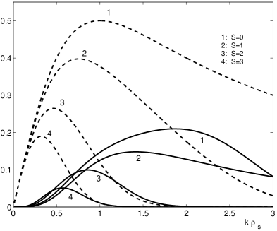
Figure 1: The frequencies (dashed curves) and the growth rates of drift modes for several values of the size of trajectory structures

The growth rate of the drift modes for different values of the size $\overline{s}$ of the trajectory structures is shown in Figure 1. This shows that the range of the wave numbers for the unstable test modes is displaced toward small $k_{\perp}.$ This determines a further increase of the size of trajectory structures. The diffusive term in (48) lead to the damping of the modes with $\overline{k}_{\perp}\gg 1/\overline{s}.$

This means that EC of the turbulence evolves in this weakly nonlinear stage by increasing its amplitude $\beta$ and by increasing the correlation length and the average wave number $k_{0}$ (32). The vortical structures of ion trajectories produced by trapping determine this processes.

6 Ion flows and turbulence attenuation

The evolution of the potential determines the increase of the fraction of trapped ions. This determines an average flux of the trapped particles that move with the potential $n_{tr}V_{\ast e}.$ As the $\mathbf{E}\times\mathbf{B}$ drift has zero divergence, the probability of the Lagrangian velocity is time invariant, i. e. it is the same with the probability of the Eulerian velocity. The average Eulerian velocity is zero and thus the flux of the trapped ions that move with the potential has to be compensated by a flux of the free particles. These particles have an average motion in the opposite direction with a velocity $V_{f}$ such that

$$n_{tr}V_{\ast e}+n_{f}V_{f}=0.$$ (49)

The NSA shows that the probability of the displacements splits in two components that move in opposite direction. The peak of trapped ions moves with the velocity $V_{\ast e}$ while the free ions move in the opposite direction with a velocity that increases with the increase of the fraction of trapped ions. The distribution of trapped ions is almost frozen while that of free ions has a continuously growing width. Thus, opposite ion flows are generated by the moving potential in the presence of trapping. A simple approximation that includes the main features of the distribution is

$$P(x,y,t)=n_{tr}G(x,y-V_{\ast e}t;S_{x},S_{y})+n_{f}G(x,y-V_{f}t;S_{x}^{\prime},S_{y}^{\prime}).$$ (50)

where two Gaussian functions were used as in Eq. (43) but taking into account the ion flows (49). The average velocity of the free ions is $V_{f}=-nV_{\ast e},~{}$where $n=n_{tr}/n_{f}.$ The separation of the distribution and the existence of ion flows in drift type turbulence are confirmed by numerical simulations [14].

The compressibility term $L_{i}$ (29) is determined for trapped and free particles with the DTM. It can be written as

$$L_{x}=-\frac{V_{\ast e}}{\Omega_{i}B^{2}}\int_{\tau}^{t}d\tau^{\prime\prime}\int_{\tau}^{t}d\tau^{\prime}\left\langle\partial_{y}\phi\left(\mathbf{x}(\tau^{\prime\prime})\right)~{}\partial_{y}\Delta\phi\left(\mathbf{x}(\tau^{\prime})\right)\right\rangle.$$

A nonzero value is obtained for $L_{x}$ essentially because the potential and the Laplacean of the potential are correlated in a stochastic field: the maxima of the potential statistically coincide with the minima of the Laplacean. It follows that the derivatives of these functions along the same directions are also correlated and the derivatives on different directions are not. Indeed, one obtains from Eq. (32)

$$\left\langle\partial_{x}\phi\left(\mathbf{x}\right)~{}\partial_{y}\Delta\phi\left(\mathbf{x}\right)\right\rangle = -\partial_{x}\partial_{y}\Delta E(\mathbf{0})=0$$ (51)

$$\left\langle\partial_{y}\phi\left(\mathbf{x}\right)~{}\partial_{y}\Delta\phi\left(\mathbf{x}\right)\right\rangle = -\partial_{y}^{2}\Delta E(\mathbf{0})=-\frac{\beta^{2}}{\lambda^{4}}c,$$ (52)

where

$$c=\left(\frac{k_{0}^{2}+3}{\delta}+15+10~{}k_{0}^{2}+k_{0}^{4}\right)$$ (53)

The corresponding Lagrangian correlations are determined with the DTM. The component $L_{y}$ is zero for both trapped and free ions due to the symmetry of the correlation (51). $L_{x}$ is different for free and trapped trajectories. In the first case there is a relative motion of the free ions and of the potential with the velocity $V_{\ast e}/n_{f}$ (obtained from (49)), which determines rapid decorrelation. The estimation done for the quasilinear turbulence also holds in these conditions and $L_{x}$ for free ions is approximated by Eq. (35) with $V_{\ast e}$ replaced by $V_{\ast e}/n_{f},~{}$and thus it is negligible. For the trapped trajectories, $L_{x}$ is much larger than in the quasilinear case. It can be determined with the DTM, which shows that the following estimation holds.

$$L_{x}(\tau,t)=-\frac{V_{\ast e}}{\Omega_{i}B^{2}}\int_{\tau}^{t}d\tau^{\prime\prime}\int_{\tau}^{t}d\tau^{\prime}C_{x}\left(\left|\tau^{\prime\prime}-\tau^{\prime}\right|\right),$$

$$C_{x}\left(\left|\tau^{\prime\prime}-\tau^{\prime}\right|\right)=\left\langle\partial_{y}\phi\left(\mathbf{x}(\tau^{\prime\prime})-V_{\ast e}(t-\tau^{\prime\prime})\right)~{}\partial_{y}\Delta\phi\left(\mathbf{x}(\tau^{\prime})-V_{\ast e}(t-\tau^{\prime})\right)\right\rangle.$$

The integral is calculated by changing the integration variable $\tau^{\prime\prime}$ to $\theta=\tau^{\prime\prime}-\tau^{\prime}$

$$L_{x}(\tau,t)=-\frac{2V_{\ast e}}{\Omega_{i}B^{2}}\int\limits_{0}^{t-\tau}d\theta C_{x}\left(\left|\theta\right|\right)\left(t-\tau-\theta\right),$$

which integrated by parts gives

$$L_{x}(\tau,t)=-\frac{2V_{\ast e}}{\Omega_{i}B^{2}}\int\limits_{0}^{t-\tau}d\theta~{}\emph{J}\left(\theta\right)$$

where

$$\emph{J}\left(\theta\right)=\int\limits_{0}^{\theta}d\tau C_{x}\left(\tau\right).$$

This function saturates after the decorrelation time $\tau_{d}$ at $\emph{J}\left(\theta\right)=C_{x}\left(0\right)\tau_{d}.$ In these conditions of strong turbulence, the decorrelation time for the $C_{x}$ is, as for the correlation of the stochastic $\mathbf{E\times B}$ velocity, the time of flight $\tau_{fl}.$ Thus

$$L_{x}(\tau,t)\cong a\left(t-\tau\right),\ \ \ a=2\partial_{y}^{2}\Delta E(\mathbf{0})\frac{\tau_{fl}V_{\ast e}}{\Omega_{i}B^{2}},$$ (54)

where $a$ has the dimension of a velocity. This type of Lagrangian correlation corresponds to the decorrelation by mixing.

Thus, the compressibility of the background turbulence is correlated with the displacements along $x$ and influences the propagator for the trapped ions. The function $M$ (28) that accounts for the effects of the background turbulence is determined using Eqs. (50) and (54)

$$M = n_{f}\exp\left[-\frac{k_{i}^{2}}{2}\left(S_{i}^{2}+2D_{i}(t-\tau)\right)-ik_{y}V_{f}(t-\tau)\right]+$$ (55)

$$n_{tr}\exp\left[-\frac{k_{i}^{2}}{2}S_{i}^{2}-ik_{y}V_{\ast e}(t-\tau)+ik_{x}a(t-\tau)\right].$$

The average propagator (27) becomes in these conditions

$$\overline{\Pi}^{i}=-\mathcal{F}\left[\frac{n_{f}}{\omega-k_{y}V_{f}}+\frac{n_{tr}}{\omega-k_{y}V_{\ast e}+k_{x}a}-ik_{i}^{2}D_{i}\frac{n_{f}}{\left(\omega-k_{y}V_{f}\right)^{2}}\right]$$ (56)

where the fact that the diffusion term is small was used.

The dispersion relation is

$$\mathcal{F}~{}\left(k_{y}V_{\ast e}-\omega k^{2}\rho_{s}^{2}\right)\left[\frac{n_{f}}{\omega-k_{y}V_{f}}+\frac{n_{tr}}{\omega-k_{y}V_{\ast e}+k_{x}a}-i\frac{k_{i}^{2}D_{i}n_{f}}{\left(\omega-k_{y}V_{f}\right)^{2}}\right]$$ (57)

$$= 1+i\sqrt{\frac{\pi}{2}}\frac{\omega-k_{y}V_{\ast e}}{\left|k_{z}\right|v_{Te}}$$

The compressibility term $k_{x}a$ competes with the term $\omega-k_{y}V_{\ast e}$ that is of the order $k_{y}V_{\ast e}$. Its effect is measured by the ratio

$$r=\frac{k_{x}a}{k_{y}V_{\ast e}}=2c\sqrt{\frac{\alpha}{k_{0}^{2}+3}}\frac{k_{x}}{k_{y}}\frac{\rho_{s}}{\lambda}\frac{V}{c_{s}}$$ (58)

where $c$ is the normalized correlation (53). For a typical plasma with $c_{s}=10^{6}m/s,$ $\beta=150V,$ $B=3T,$ $\lambda=10^{-2}m,$ $\rho_{s}=2~{}10^{-3},$ one obtains $V/c_{s}=5~{}10^{-3}.$ The correlation $c\geq 20$, which leads to $r\cong 0.05$ for $k_{y}\cong k_{x}.$ It means that the compressibility term can be neglected for modes with $k_{y}$ larger or of the order of $k_{x}$ and that it is important for modes with $k_{y}\rightarrow 0.$

The solution of the dispersion relation is determined for the two cases: $k_{y}\gtrsim k_{x}$  that corresponds to drift modes and $k_{y}=0,$ which are modes with different characteristics called zonal flow modes.

6.1 Drift modes

Neglecting the compressibility term $\left(a=0\right)$, the real part of the dispersion relation (57) is

$$\mathcal{F}\left(\overline{k}_{y}-\overline{\omega}_{d}\overline{k}_{\perp}^{2}\right)\left[\overline{\omega}_{d}+\left(n-1\right)\overline{k}_{y}\right]=\left(\overline{\omega}_{d}+n\overline{k}_{y}\right)\left(\overline{\omega}_{d}-\overline{k}_{y}\right),$$ (59)

where the suscript was introduced in $\overline{\omega}_{d}$ to account for drift type modes. Taking $\overline{\omega}_{d}=\overline{\omega}_{0}+\overline{\delta}(n,k),$ where $\overline{\omega}_{0}=\mathcal{F}\overline{k}_{y}/\left(1+\mathcal{F}\overline{k}_{\perp}^{2}\right)$ is the frequency (47) in the absence of ion flows $(n=0),$ the equation becomes

$$\overline{\delta}\left[\overline{\delta}+\overline{\omega}_{0}+\left(n-1\right)\overline{k}_{y}\right]=\frac{n\overline{k}_{y}^{2}}{1+\mathcal{F}\overline{k}_{\perp}^{2}},$$ (60)

where Doppler shift with the velocity of the trapped and free ions appears in the parenthesis in the left side term, $\omega_{0}-k_{y}V_{f}-k_{y}V_{\ast e}=k_{y}V_{\ast e}\left[\overline{\omega}_{0}+\left(n-1\right)\overline{k}_{y}\right].$ The solutions are the two intersections of the parabola in the left hand side of Eq. (60) with the horizontal line at the level $n\overline{k}_{y}^{2}/\left(1+\mathcal{F}\overline{k}_{\perp}^{2}\right).$ The condition $\overline{\delta}=0$ for $n=0$  chooses one of the two solutions, namely on the branch of the parabola that passes through the origin. This leads to $\overline{\delta}<0$ if $\overline{\omega}_{0}+\left(n-1\right)\overline{k}_{y}<0$ and $\overline{\delta}>0$ if $\overline{\omega}_{0}+\left(n-1\right)\overline{k}_{y}>0.$ The absolute value of $\overline{\delta}$ is an increasing function of $n$ in both cases, and thus, as $n$ increases, the decrease of $\overline{\omega}_{d}$ is produced by the ion flows in the first case and the increase of $\overline{\omega}_{d}$ in the second case. The solution of the dispersion relation (59) is

$$\overline{\omega}_{d}=\frac{1}{2}\left[\overline{\omega}_{0}+\left(1-n\right)\overline{k}_{y}+sg\sqrt{\left[\overline{\omega}_{0}+\left(n-1\right)\overline{k}_{y}\right]^{2}+\frac{4n\overline{k}_{y}^{2}}{1+\mathcal{F}\overline{k}_{\perp}^{2}}}\right],$$

where $sg=sign\left[\overline{\omega}_{0}+\left(n-1\right)\overline{k}_{y}\right].$ A jump appears in the frequency at the value of $k_{d}$ determined by the equation $\overline{\omega}_{0}=\left(1-n\right)\overline{k}_{y},$ which has solution if $n<1.$ $k_{d}$ is an increasing function of $n.$In the limit of large $k,$ $\overline{\omega}_{d}\rightarrow-n\overline{k}_{y}$ if $n<1$ and $\overline{\omega}_{d}\rightarrow\overline{k}_{y}$ if $n>1.$ This means that the asymptotic phase velocity is in the ion diamagnetic direction when $n<1$ and in the electron diamagnetic direction when trapping is stronger such that $n>1.$

The imaginary part (obtained using the condition $\overline{\gamma}_{d}\ll\overline{\omega}_{d})$ is

$$\overline{\gamma}_{d}\mathcal{F}\left[\left(1-\overline{\omega}_{d}\ \overline{k}_{\perp}^{2}\right)f_{+}+\overline{k}_{\perp}^{2}\left(\frac{n_{f}}{\overline{\omega}_{d}+n\overline{k}_{y}}+\frac{n_{tr}}{\overline{\omega}_{d}-\overline{k}_{y}}\right)\right]$$

$$= \gamma_{0}\left(\overline{k}_{y}-\overline{\omega}_{d}\right)-n_{f}\overline{k}_{i}^{2}\overline{D}_{i}\frac{\mathcal{F}\left(1-\overline{\omega}_{d}\overline{k}_{\perp}^{2}\right)}{\left(\overline{\omega}_{d}+n\overline{k}_{y}\right)^{2}}$$

where

$$f_{+}=\left(\frac{n_{f}}{\left(\overline{\omega}_{d}+n\overline{k}_{y}\right)^{2}}+\frac{n_{tr}}{\left(\overline{\omega}_{d}-\overline{k}_{y}\right)^{2}}\right)>0.$$

Using (59), the solution can be written as

$$\overline{\gamma}_{d}=\frac{\gamma_{0}\left(\overline{\omega}_{d}+n\overline{k}_{y}\right)\left[\left(1-n\right)\overline{k}_{y}-\overline{\omega}_{d}\right]-n_{f}\overline{k}_{i}^{2}\overline{D}_{i}}{\left[\left(1-n\right)\overline{k}_{y}-\overline{\omega}_{d}\right]^{2}\left(1+\mathcal{F}\overline{k}_{\perp}^{2}\right)+n\overline{k}_{y}^{2}}\left(\overline{k}_{y}-\overline{\omega}_{d}\right)^{2}.$$ (61)

The growth rates are presented in Figure 2a. The jump in the frequency corresponds to a jump in the growth rate from negative (at small $k$) to positive values. Thus the large wave-length modes are stabilized by the ion flows, while the small wave-length modes still grow. This leads to the increase of the amplitude of turbulence accompanied by the decrease of its correlation length. Both effects contribute to the increase of the ratio $\tau_{\ast}/\tau_{fl}=\beta/(V_{\ast e}\lambda_{y}B),$ which leads to the increase of $n$. Consequently, the increase of the amplitude of the turbulence continues as well as the damping of small $k$ modes and the decrease of the correlation length. The process is stopped when $n>1$ because the growth rate becomes negative for the whole wave number range. This determines the decrease of $n$ and the attenuation of the ion flows.

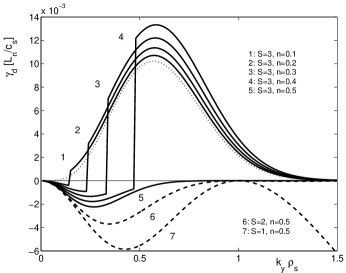
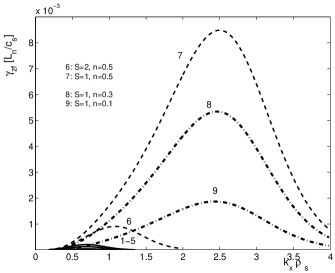
Figure 2: Growth rate dependence on the fraction of trapped ions $n$ and on the size $S$ of trajectory structures for drift modes (left panel) and zonal flow modes (right panel). The curves with the same label correspond to the same parameters.

6.2 Zonal flow modes ($k_{y}=0)$

The compressibility term becomes dominant for $k_{y}=0.$ As shown below it determines unstable modes completely different of the drift modes: with $k_{y}=0,$ $k_{x}\neq 0$ and very small frequency $\omega_{zf}$, much smaller than the diamagnetic frequency. These are zonal flow modes.

The dispersion relation for $k_{y}=0$ is

$$-\omega_{zf}\mathcal{F}k_{x}^{2}\rho_{s}^{2}\left[\frac{n_{f}}{\omega_{zf}+ik_{i}^{2}D_{i}}+\frac{n_{tr}}{\omega_{zf}+k_{x}a}\right]=1+i\sqrt{\frac{\pi}{2}}\frac{\omega_{zf}}{\left|k_{z}\right|v_{Te}},$$

For $\gamma_{zf},$ $k_{i}^{2}D_{i}\ll\omega_{zf},$ the real part is

$$-\omega_{zf}\mathcal{F}k_{x}^{2}\rho_{s}^{2}\left(\omega_{zf}+n_{f}k_{x}a\right)=\omega_{zf}\left(\omega_{zf}+k_{x}a\right)$$

with the solution

$$\overline{\omega}_{zf}=-\overline{k}_{x}\overline{a}\frac{1+\mathcal{F}\overline{k}_{x}^{2}n_{f}}{1+\mathcal{F}\overline{k}_{x}^{2}}$$ (62)

where

$$\overline{a}=\frac{a}{V_{\ast e}}=2c\sqrt{\frac{\alpha}{k_{0}^{2}+3}}\frac{\rho_{s}}{\lambda}\frac{V}{c_{s}}$$

The imaginary part is

$$\gamma_{zf}\mathcal{F}k_{x}^{2}\rho_{s}^{2}\left[\omega_{zf}\left(\frac{n_{f}}{\omega_{zf}^{2}}+\frac{n_{tr}}{\left(\omega_{zf}+k_{x}a\right)^{2}}\right)-\frac{n_{f}}{\omega_{zf}}-\frac{n_{tr}}{\omega_{zf}+k_{x}a}\right]$$

$$= \sqrt{\frac{\pi}{2}}\tau_{\parallel e}\omega_{zf}-k_{x}^{4}D_{x}\mathcal{F}\rho_{s}^{2}\frac{n_{f}}{\omega_{zf}}$$

with the solution

$$\overline{\gamma}_{zf}=\left[\gamma_{0}\left(\overline{k}_{x}\overline{a}\right)^{2}\frac{\left(1+n_{f}\mathcal{F}\overline{k}_{x}^{2}\right)^{2}}{\left(1+\mathcal{F}\overline{k}_{x}^{2}\right)^{2}}-n_{f}\mathcal{F}\overline{k}_{x}^{4}\overline{D}_{x}\right]\frac{n_{tr}\mathcal{F}\overline{k}_{x}^{2}}{\left(1+n_{f}\mathcal{F}\overline{k}_{x}^{2}\right)\left(1+\mathcal{F}\overline{k}_{x}^{2}\right)}$$ (63)

These unstable zonal flow modes are consequence of trapping combined with the polarization drift. One can see that when trapping is negligible ($n_{tr}\cong 0),$ $\omega_{zf}=-k_{x}a$ and $\gamma_{zf}=0,$ and that $\omega_{zf},\gamma_{zf}=0$ for $\overline{a}=0.$ As seen in Figure 2b, the growth rate of zonal flows is positive and it increases with the increase of $n_{tr}$ and with the decrease of the size of the trajectory structures.

Thus we have shown that zonal flow modes are generated due to ion flows. They have positive growth rates and small frequencies (typically ten times smaller than the diamagnetic frequency).

In conclusion, the ion flows produced by ion trapping in the moving potential determine two parallel effects: nonlinear damping of drift modes and generation of zonal flow modes. There is no causality relation between zonal flow modes and drift turbulence damping. Both effects are generated selfconsistently in the nonlinear evolution of drift turbulence. The influence produced by the zonal flows on the drift type modes is only indirect, through the diffusive damping. Zonal flows modify the configuration of the potential and consequently the correlation of the turbulence by introducing components with $k_{y}\cong 0$ in the spectrum, which change the shape of the EC. The integral of the EC along $y$ becomes finite. This determines a rather strong increase of the diffusion coefficient $D_{y},$ which contribute to the decay of the drift type turbulence. Zonal flow modes also modify the diffusion along $x$ but in the opposite sense: a strong decrease appears due to the decrease of $\lambda_{x}$ produced by the zonal flow component of the turbulence. The drift turbulence decay determines the decrease of $n_{tr},$ which reduces the growth rate of zonal flow modes.

There is time correlation between the maximum growth rate of zonal flow modes and the damping of the drift modes, as observed in experiments and in the numerical simulations. This time correlation can be deduced from Figures 2 (a, b), which show the growth rates of the drift and zonal flow modes for the same set of parameters $n,\ S.$ When the drift turbulence amplitude increases determining the increase of the fraction $n$ of trapped ions (curves 1-5) the growth rate of the zonal flows is very small. When the growth rate of the drift modes becomes negative and the size of the ion trajectory structures decreases (curves 6, 7 in Figure 2) the growth rate of the zonal flow modes strongly increases and, at small $S,$ it becomes comparable with that of the drift modes. The attenuation of the drift turbulence that leads to the decrease of $n$ determines the decrease of the growth rate of the zonal flow modes (curves 8, 9 in Figure 2 b).

We note that the effect of ion diffusion on the zonal flow modes and of drift modes is different. Ion diffusion determines the damping of the drift modes with large $k.$ This effect is well known and appears on the whole evolution of the drift modes, from the quasilinear to the strongly nonlinear stage characterized by the existence of ion flows. In the case of zonal flow modes, Eq. (LABEL:gamzf) shows that the effect of ion diffusion on large $k_{x}$ modes is negligible due to the factor $\mathcal{F}$ that goes to zero. The diffusion has strongest effect on the modes with $k_{x}\cong\sqrt{1/S_{x}},$ and it can even determine negative $\gamma$ at small $k_{x}.$

The evolution of the turbulence in this strongly nonlinear stage is rather complex. The ion flows determine first the increase of the amplitude of the turbulence and the decrease of the correlation length $\lambda_{y}$, then a major modification of the EC shape appears due to generation of zonal flow modes and eventually the turbulence is strongly attenuated. The new component that accounts for the zonal flow modes adds to the EC a function with a slow decay along $y$ ($k_{y}\cong 0),$ with zero integral along $x$ (because $\gamma=0$ for $k_{x}=0)$ and with amplitude growing with the increase of $n.$ It essentially determines in the total EC the increase of $\lambda_{y}$ and of the amplitude $\beta$ and the decrease of $\lambda_{x}.$

7 Summary and conclusions

Test modes on turbulent plasmas were studied taking into account the process of ion trajectory trapping in the structure of the background potential. The case of drift turbulence was considered, and the frequency $\omega$ and the growth rate $\gamma$ were determined as functions of the statistical properties of the background turbulence. The main characteristics of the evolution of the turbulence were deduced from $\gamma$ and $\omega.$

A different physical perspective on the nonlinear evolution of drift turbulence is obtained.

The main role is played by the trapping of the ions in the stochastic potential that moves with the diamagnetic velocity. The fraction of trapped ions is a function of $K_{\ast}=\beta/(\lambda_{x}V_{\ast e}B).$ Trapping appears for $K_{\ast}>1$ and the fraction of trapped trajectories $n_{tr}$ increases with the increase of this parameter. Trapped trajectories form quasi-coherent structures, which determine non-Gaussian distribution of the displacements. At larger amplitudes, the moving potential determines ion local flows: the trapped ions move with the potential while the other ions drift in the opposite direction. These opposite (zonal) flows compensate such that the average ion velocity is zero, but they determine the spliting of the distribution of displacements.

The first effect of trapping in turbulence evolution appears when the fraction of trapped ions is small and the ion flows are negligible. The trapped ions determine the evolution of the turbulence toward large wave lengths (the inverse cascade).

The influence of the ion flows produced by the moving potential appears later in the evolution of the turbulence when the fraction of trapped ions is comparable whith that of free ions. The ion flows determine first the damping of the small $k_{\perp}$ drift modes and eventually the damping of the drift modes with any $k_{\perp}.$ In the same time, trapping in connection with the compressibility produced by the polarization drift in the background turbulence determine transitory zonal flow modes (with $k_{y}=0$ and $\omega\ll k_{y}V_{\ast e}).$ Thus, in this perspective, there is no causality connection between the damping of the drift turbulence and the zonal flow modes. Both processes are produced by ion trapping in the moving potential.

During the decay of the turbulence trapping is maintained because the decrease of the amplitude is compensated by decrease of the correlation length, leading to small variations of the parameter $K_{\ast}$. The damping is first produced for the small wave numbers and thus there is a transitory domination by large wave numbers in the spectrum. This determines a hysteresis process: the growth and the decay of the turbulence is produced on different paths. Large scales are generated at the development (increase) of the turbulence and the correlation length increases. This determines only a slow increase of the parameter $K_{\ast}$ and thus a slow increase of the number of trapped trajectories $n_{tr}.$Then, the ion flows become important and produce further increase of the larger part of the wave number spectrum accompanied by the decay of the small $k$ modes. Thus, the amplitude of the potential increases and the correlation length decrease. This determines a much faster increase of $K_{\ast}$ and of the relative number of trapped ions. When the latter is $n_{tr}=0.5,$ the growth rates of all drift modes are negative and the amplitude of the turbulence decays leading to the decrease of $n_{tr}$. This process continues until the ion flows become negligible ($n_{tr}\ll n_{f}).$ A closed evolution curve in the $\left(\beta,~{}\lambda\right)$ space is described by the turbulence, which remains in the nonlinear stage characterized by trapping and oscillates between weak and strong trapping.

The zonal flows appear due to ion flows as well as turbulence nonlinear damping. The damping process is not determined by the zonal flows. There is however an influence produced by the zonal flows on the drift type modes. It is not direct but through the diffusive damping. Zonal flows modify the correlation of the turbulence by introducing components with $k_{y}=0$ in the spectrum. This changes the shape of the EC, which has no more zero integral along the $y$ direction. This determines the increase of the diffusion $D_{y},$ which contribute to the decay drift type turbulence but not of the zonal flow modes.

The diffusion coefficient along $x$ axis also oscillates during the evolution of the turbulence. Its maximum is correlated with the period when the correlation lengths along $x$ is large, which appears before the development of the ion flows.

The zonal flow modes increase and drift turbulence decay appear to be temporally correlated, as observed in experiments and simulations. The characteristic time $\Delta t$ for turbulence and transport oscillations can be estimated as the inverse of the growth rates, which are of the order of $5\ 10^{-3}c_{s}/L_{n}.$ One obtains for $L_{n}/R_{0}=5,$ $\Delta t=40\ R_{0}/c_{s},$ in agreement with the numerical simulations.

This work was supported by CNCSIS-UEFISCDI, project number PNII - IDEI 1104/2008.

References

- [1] Krommes J. A., Phys. Reports 360 (2002) 1.
- [2] Horton W, Rev. Modern Phys. 71 (1999) 735.
- [3] Garbet X, Idomura Y, Villard L, Watanabe T H, Nuclear Fusion 50 (2010) 043002.
- [4] Tynan G. R., Fujisawa A., McKee G., Plasma Phys. Control. Fusion 51 (2009) 113001.
- [5] Terry PW, Rev. Mod. Phys. 72, 109 (2000)
- [6] Diamond P. H., Itoh S.-I., Itoh K., Hahm T. S., Plasma Phys. Control. Fusion 47 (2005) R35-R161.
- [7] Vlad M., Spineanu F., Misguich J.H., Balescu R., Phys.Rev.E 58 (1998) 7359.
- [8] Vlad M. and Spineanu F., Phys. Rev. E 70 (2004) 056304.
- [9] Dupree T. H., Phys. Fluids 9 (1966) 1773.
- [10] Dupree T. H., Phys. Fluids 15 (1972) 334.
- [11] Spineanu F., Vlad M., Phys. Letters A 133 (1988) 319.
- [12] Vlad M., Spineanu F., Misguich J.H., Plasma Phys. Control. Fusion 36 (1994) 95.
- [13] Goldstone R. J. and Rutherford P. H., Introduction to Plasma Physics, Institute of Physics Publishing, Bristol and Philadelphia, 1995.
- [14] Hauff T, Jenko F, Phys. Plasmas 14 (2007) 092301.
- [15] R. H. Kraichnan, Phys. Fluids 19, 22 (1970).
- [16] Balescu R., Aspects of Anomalous Transport in Plasmas, Institute of Physics Publishing (IoP), Bristol and Philadelphia, 2005.
- [17] W. D. McComb, The Physics of Fluid Turbulence (Clarendon, Oxford, 1990).
- [18] Vlad M., Spineanu F., Misguich J. H. and Balescu R., Phys. Rev. E 61 (2000) 3023.
- [19] Vlad M., Spineanu F., Misguich J. H. and Balescu R., Phys. Rev. E 63 (2001) 066304.
- [20] Vlad M., Spineanu F., Misguich J. H. and Balescu R., Nuclear Fusion 42 (2002) 157.
- [21] Vlad M., Spineanu F., Misguich J. H., Reusse J.-D., Balescu R., Itoh K., Itoh S.-I., Plasma Phys. Control. Fusion 46 (2004) 1051.
- [22] Petrisor I., Negrea M., Weyssow B., Physica Scripta 75 (2007) 1.
- [23] Vlad M., Spineanu F., Misguich J.H., Balescu R., Phys. Rev. E 67 (2003) 026406.
- [24] Neuer M., Spatschek K. H., Phys. Rev. E 74 (2006) 036401.
- [25] Vlad M., Spineanu F., Benkadda S., Phys. Rev. Letters 96 (2006) 085001.