Safe and Stabilizing Distributed Multi-Path Cellular Flows
Abstract
We study the problem of distributed traffic control in the partitioned plane, where the movement of all entities (robots, vehicles, etc.) within each partition (cell) is coupled. Establishing liveness in such systems is challenging, but such analysis will be necessary to apply such distributed traffic control algorithms in applications like coordinating robot swarms and the intelligent highway system. We present a formal model of a distributed traffic control protocol that guarantees minimum separation between entities, even as some cells fail. Once new failures cease occurring, in the case of a single target, the protocol is guaranteed to self-stabilize and the entities with feasible paths to the target cell make progress towards it. For multiple targets, failures may cause deadlocks in the system, so we identify a class of non-deadlocking failures where all entities are able to make progress to their respective targets. The algorithm relies on two general principles: temporary blocking for maintenance of safety and local geographical routing for guaranteeing progress. Our assertional proofs may serve as a template for the analysis of other distributed traffic control protocols. We present simulation results that provide estimates of throughput as a function of entity velocity, safety separation, single-target path complexity, failure-recovery rates, and multi-target path complexity.
keywords:
distributed systems , swarm robotics , formal methods1 Introduction
Highway and air traffic flows are nonlinear switched dynamical systems that give rise to complex phenomena such as abrupt phase transitions from fast to sluggish flow [1, 2, 3]. Our ability to monitor, predict, and avoid such phenomena can have a significant impact on the reliability and capacity of physical traffic networks. Traditional traffic protocols, such as those implemented for air traffic control are centralized [4]—a coordinator periodically collects information from the vehicles, decides and disseminates waypoints, and subsequently the vehicles try to blindly follow a path to the waypoint. Wireless vehicular networks [5, 6, 7, 8] and autonomous vehicles [9, 10] present new opportunities for distributed traffic monitoring [11, 12, 13] and control [14, 15, 16, 17, 18, 19]. While these protocols may still rely on some centralized coordination, they should scale and be less vulnerable to failures compared to their centralized counterparts. In this paper, we propose a fault-tolerant distributed traffic control protocol, formally model it, and formally prove its correctness.
A traffic control protocol is a set of rules that determines the routing and movement of certain physical entities, such as vehicles, robots, or packages, over an underlying graph, such as a road network, air-traffic network, or warehouse conveyor system. Any traffic control protocol should guarantee: (a) (safety) that the entities always maintain some minimum physical separation, and (b) (progress) that the entities eventually arrive at a given a destination (or target) vertex. In a distributed traffic control protocol, each entity determines its own next-waypoint, or each vertex in the underlying graph determines the next-waypoints for the entities in an appropriately defined neighborhood.
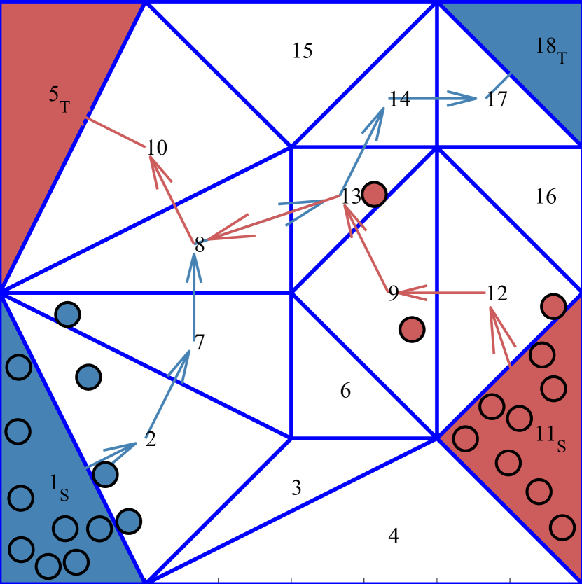
In this paper, we study the problem of distributed traffic control in a partitioned plane where the motions of entities within a partition are coupled. The problem can be described as follows (refer to Figures 2 and 2). The environment—the geographical space of interest—is partitioned into regions or cells. Each entity is assigned a certain type or color. For each color, there is one source cell and one target cell of the same color. The source cells produce entities of some color, and the target cells only consume entities of a particular color, so the goal is to move entities of color to the target of color . The motion of all entities within a cell are coupled, in the sense that they all either move identically, or they all remain stationary (we discuss the motivation for this below). If some entities within some cell touch the boundary of a neighboring cell , those entities are transferred to . Thus, the role of the distributed traffic control protocol is to control the motion of the cells so that the entities (a) always have the required safe separation, and (b) reach their respective targets, when feasible.
The coupling mentioned above that requires entities within a cell to move identically may appear strong at first sight. After all, under low traffic conditions, individual drivers control the movement of their cars within a particular region of the highway, somewhat independently of the other drivers in that region. However, on highways under high-traffic, high-velocity conditions, it is known that coupling may emerge spontaneously, causing the vehicles to form a fixed lattice structure and move with near-zero relative speed [1, 20]. In other scenarios, coupling arises because passive entities are moved around by active cells. For example, this occurs with packages being routed on a grid of multi-directional conveyors [21, 22], and molecules moving on a medium according to some controlled chemical gradient. Finally, even where the entities are active and cells are not, the entities can cooperate to emulate a virtual active cell expressly for the purposes of distributed coordination. This idea has been explored for mobile robot coordination in [23] using a cooperation strategy called virtual stationary automata [24, 25].
In this paper, we present a distributed traffic control protocol that guarantees safety at all times, even when some cells fail permanently by crashing. The protocol also guarantees eventual progress of entities toward their targets, provided (a) that there exists a path through non-faulty cells to the entities’ respective targets, and (b) failures have not introduced unrecoverable deadlocks. Specifically, the protocol is self-stabilizing [26, 27], in that once new failures stop occurring, the composed system automatically returns to a state from which progress can be made. The algorithm relies on the following four mechanisms.
-
(a)
There is a routing rule to maintain local routing tables to each target at each non-faulty cell. This routing protocol is self-stabilizing and allows our protocol to tolerate crash failures of cells.
-
(b)
There is a mutual exclusion and scheduling mechanism to ensure moving entities over distinctly colored overlapping paths do not introduce deadlocks. The locking and scheduling mechanism ensures one-way traffic can make progress over shared routes (traffic intersections).
-
(c)
There is a signaling rule between neighbors that guarantees safety while preventing deadlocks. Roughly speaking, the signaling mechanism at some cell fairly chooses among its neighboring cells that contain entities, indicating if it is safe for one of these cells to apply a movement in the direction of the cell doing the signaling. This permission-to-move policy turns out to be necessary, because movement of neighboring cells may otherwise result in a violation of safety in the signaling cell, if entity transfers occur.
-
(d)
The movement policy causes all entities on a cell to either move with the same constant velocity in the direction of their destination, or remain stationary to ensure safety. This policy abstracts more complex motion modeling.
We establish these safety and progress properties through systematic assertional reasoning. For safety properties, we establish inductive invariants and for stabilization we use global ranking functions. To show that all entities reach their destinations (when feasible), we use a combination of ranking functions and fairness-based reasoning on infinite executions. These proof techniques may serve as a template for the analysis of other distributed traffic control protocols. Our analysis is generally independent of the size of the environment, number of cells, and number of entities. Additionally, only neighboring cells communicate with one another and the communication topology is fixed (aside from failures). For these reasons, this problem can serve as a case study in automatic parameterized verification of distributed cyber-physical systems [28, 29, 30, 31].
We present simulation results that illustrate the influence (or the lack thereof) of several factors on throughput. (a) Throughput decreases exponentially with path length until saturation, as which point it decreases roughly linearly with path length. (b) Throughput decreases roughly linearly with required safety separation and cell velocity. (c) Throughput decreases roughly exponentially until it saturates as a function of path complexity measured in number of turns along a path. (d) Throughput decreases roughly exponentially with failure rate, and increases linearly with recovery rates, under a model where crash failures are not permanent and cells may recover from crashing. (e) Throughput decreases roughly exponentially until it saturates as a function of the percentage of overlapping cells between different colored targets.
Contributions over Previous Work
In previous work [32], we analyzed a similar problem, but have significantly generalized our results in this paper.
-
(A)
We consider general tessellations (including triangulations) that define the partitioning, while we considered uniform square partitions in [32]. We also present results on partitioning schemes that cannot work for our formulation of the problem.
-
(B)
We allow entities of multiple colors, each flowing to a different target, while in [32], we only allowed entities of one color, all of which flowed to the nearest target. This generalization lets source-to-target paths of different colors overlap, creating intersections, and requires several changes to the algorithm, including adding a mutual exclusion and scheduling mechanisms used to control traffic intersections. This generalization is significant because it makes the problem applicable to a much wider class of systems.
-
(C)
We extended our simulation results to allow for these generalizations, and characterized the cost on throughput due to the extra coordination required to allow multiple colors.
Paper Organization
The rest of the paper is organized as follows. First, Section 2 introduces the model of the physical system. Next in Section 3, we present the distributed traffic control algorithm. Then in Section 4, we define and prove the safety and progress properties. Subsection 4.1 establishes safety. Subsequently, we establish a progress property that shows entities eventually reach their targets in spite of failures (when possible). First in Subsection 4.2, it is shown that the routing protocol to find any target from any cell with a physical path through non-faulty cells to that target is self-stabilizing. Then in Subsection 4.3, we show how overlapping paths to different targets (traffic intersections) can be scheduled. Finally, in Subsection 4.4, it is shown that entities on any cell with a feasible physical path to their target eventually reach their target. Simulation results and interpretation are presented in Section 5, followed by a brief discussion of related work and further extensions, and a conclusion in Sections 6, 7, and 8.
2 Physical System Model
We describe the physical system in this section. For a set , we define and . For , let . The brackets are used for the Euclidean norm of a vector.
Partitioning
The system consists of convex polygonal cells partitioning a polygonal environment. Let be the set of unique identifiers for all cells in the system.The planar environment is some given simply connected polygon. A partition of is a set of closed, convex polygonal cells such that:
-
(a)
the interiors of the cells are pairwise disjoint,
-
(b)
the union of the cells is the original polygonal environment, and
-
(c)
cells only touch one another at a point or along an entire side.
The first two conditions are the standard definition of a partition, while the third restricts any cell from being adjacent along one of its sides to more than one other cell. Thus, cell occupies a convex polygon in the Euclidean plane. The boundary of cell is denoted by . We denote the vertices (extreme points) of as . We denote the number of sides of as . Let be the common side of adjacent cells and —we will refer to as both an index and a line segment (set of points).
Communications
Cell is said to be a neighbor of cell if the boundaries of the cells share a common side. The set of identifiers of all neighbors of cell is denoted by . This definition of neighbors can naturally be represented as a graph, so let be the worst-case diameter of such a neighbor communication graph111The diameter of this graph is not static, it may change due to failures, but the worst case is always a path graph, so .. For each cell and each neighboring cell , let the side normal vector from to , denoted , be the unit vector orthogonal to and pointing into cell from the common side .
Each cell is controlled by software that implements the distributed traffic control algorithm described in the next section. We consider synchronous protocols that operate in rounds. At each round, each cell exchanges messages bearing state information with its neighbors. Then, each cell updates its software state and decides the (possibly zero) velocity with which to move any entities on it. Until the beginning of the next round, the cells continue to operate according to this velocity, which may lead to entity transfers.
Entities
Each cell may contain a number of entities. Each entity occupies a circular area and represents a physical object (or overapproximation of) such as an aircraft, car, robot, or package. Every entity that may ever be in the system has a unique identifier drawn from an index set . This assumption is for presentation only, and the algorithm does not rely on knowing entity identifiers. For an entity , we denote the coordinates of its center by .
The open circular area (disc) centered at of radius representing entity is denoted . The radius of an entity is , and is the minimum required inter-entity safety gap. We define the total safety spacing radius as . For simplicity of presentation, we work with uniform entity radii and safety gaps . If they differ, we would take and to be the maximums over all entities. We instantiate , which represents the physical space occupied by entity , and we also instantiate , which is entity ’s total safety area.
Entity Colors, Source Cells, and Target Cells
There are types (or colors) of entities, where is some finite, ordered set. The color of some entity is denoted as . For each , there is a source cell and a target cell . All other cells are ordinary cells. For simplicity of presentation, we assume there is a unique source and target, but the algorithms and the results generalize for when and are sets.
Entity ’s color designates the target cell entity should eventually reach. The source produces entities of color and the target consumes entities of color . The sets of target and source identifiers are denoted and , respectively.
Entity Movement
All the entities within a cell move identically—either they remain stationary or they move with some constant velocity in the direction of one of the sides of the cell. Thus is the maximum cell velocity, or the greatest distance traveled by any entity over one synchronous round. We require to ensure progress. We require that to ensure entities do not collide when transfers occur. Cell velocity may differ in each cell so long as each is upper bounded by . This movement is determined by the algorithm controlling each cell. When a moving entity touches a side of a cell, it is instantaneously transferred to the neighboring cell beyond that side, so that the entity is entirely contained in the new cell.
Safety and Transfer Regions
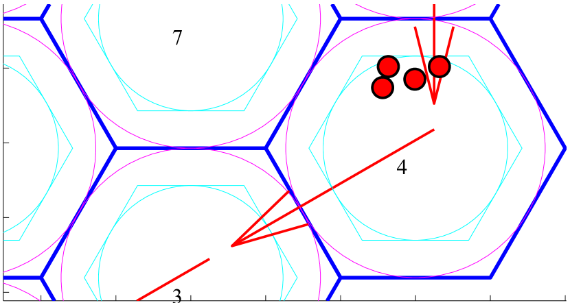
The safety region on side of a cell is the area within the cell where (the centers of) new entities entering the cell from side can be placed. For a side of some cell , the safety region on side is the area on at most distance measured orthogonally from side . Analogously, the transfer region on side of a cell is the area within a cell where (the centers of) entities reside when those entities will be transfered to the neighboring cell on that side. The transfer region on side is the region in the partition at most distance measured orthogonally from side . For a cell , the transfer region and safety region are respectively the unions of and for each side of . We refer to the inner side(s) of , , , or , as the side(s) touching the inside of the annulus, and denote them by , , etc.
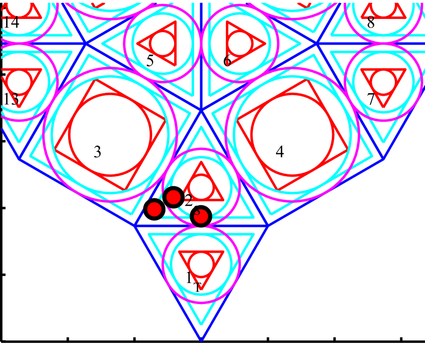
For example, in Figure 4, the transfer region for the square cell is the square annulus between the smaller cyan square and the larger blue square (the boundary of cell ). Similarly, for the triangular cell in Figure 4, the transfer region is the triangular annulus between the smaller cyan triangle and the larger blue triangle. Thus, the distance measured orthogonally between the sides of the cyan polygons representing the boundary of the transfer region, and the sides of the blue polygons is always . In Figure 4, for the square cell , the safety region is the square annulus between the smaller red square and the larger blue square.
Geometric Assumptions
We assume that the polygonal environment and its partition have shapes and sizes such that each cell in the partition is large enough for an entity to lie completely on it. Particularly, we require for each cell that the transfer region is nonempty. We also assume the following assumptions to ensure transferring entities between cells is well-defined.
Assumption 1.
(Projection Property): For each , for each side of , there exists a constant vector field over that drives every point in to some point on side without exiting .
By definition, the cells form a partition. However, partially because there is “empty space” between the transfer regions of the cells, the transfer regions do not form a partition. Even if we remove this empty space by translating the transfer regions so the sides of transfer regions of neighboring cells coincide, they still may not form a partition (see Figure 4 for an example where the transfer regions cannot form a partition). This is because, for the shared side of neighboring cells and , the inner sides of the transfer regions on and may have different lengths, even though the shared side obviously had the same length for and .
Assumption 2.
(Transfer Feasibility): For any and any , consider their common side . The length of the inner side line segment equals the length of the inner side line segment.
3 Distributed Traffic Control Algorithm
Next, we describe the discrete transition system that specifies the software controlling an individual cell of the partition .
Preliminaries
A variable is a name with an associate type. For a variable , its type is denoted by and it is the set of values that can take. A valuation (or state) for a set of variables is denoted by , and is a function that maps each to a point in . Given a valuation for , the valuation for a particular variable , denoted by , is the restriction of to . The set of all possible valuations of is denoted by . Many variables return cell identifiers that we use to access variables of other cells using subscripts, and if the valuation of these variables are restricted to the same state, we will drop the particular state on the subscripted variables for more concise notation. For instance, suppose , then would be written .
A discrete transition system is a tuple , where:
-
(i)
is a set of variables and is called the set of states,
-
(ii)
is the set of start states,
-
(iii)
is a set of transition names, and
-
(iv)
is a set of discrete transitions. For , we also use the notation .
An execution fragment of a discrete transition system is a (possibly infinite) sequence of states , such that for each index appearing in , for some . An execution is an execution fragment with . A state is said to be reachable if there exists a finite execution that ends in . is said to be safe with respect to a set if all reachable states are contained in . A set is said to be stable if, for each , implies that . is said to stabilize to if is stable and every execution fragment eventually enters .
Cells
We assume messages are delivered within bounded time and computations are instantaneous. Under these assumptions, the system can be modeled as a collection of discrete transition systems. The overall system is obtained by composing the transition systems of the individual cells. We first present the discrete transition system corresponding to each cell, and then describe the composition.
The variables associated with each are as follows, with initial values of the variables shown in Figure 7 using the ‘:=’ notation.
-
(a)
is the set of identifiers for entities located on cell . Cell is said to be nonempty if .
-
(b)
designates the entity colors on the cell, or if there are none222It will be established that cells contain entities of only a single color, see Invariant 3..
-
(c)
indicates whether or not has failed.
-
(d)
are the nonempty neighbors attempting to move entities (of any color) toward cell .
-
(e)
is a token used for fairness to indicate which neighbor may move toward .
-
(f)
is the identifier of a neighbor of that has permission to move toward .
Additionally, the following variables are defined as arrays for each color . The notation means the entry of the variable of cell , and so on for the other variables.
-
(a)
is the neighbor towards which attempts to move entities of color .
-
(b)
is the estimated distance—the number of cells—to the nearest target cell consuming entities of color .
-
(c)
is a boolean variable for a lock of color that some cells require to be able to move entities.
-
(d)
is the set of cell identifiers from any source of color (and any nonempty cell with entities of color ) to the target of color . This variable and the next two are local variables, but they are storing some global information.
-
(e)
is the set of cell identifiers in traffic intersections with cells of color (where and have nonempty intersection for some ).
-
(f)
is the set of colors that are involved in traffic intersections with the color path.
When clear from context, the subscripts in the names of the variables are dropped. A state of refers to a valuation of all these variables, i.e., a function that maps each variable to a value of the corresponding type. The complete system is an automaton, called , consisting of the composition of all the cells. A state of is a valuation of all the variables for all the cells. We refer to states of with bold letters , , etc.
⬇ 1 variables : : {} 3 : : {} , : : 5 : : : : 7 : , init , : , init , 9 : , init , : {} : , init , : {} 11 : , init , : : , init , : 13 : , init , : {} ⬇ variables 15 : : {} : : {} 17 , : : : : 19 : : : , init , 21 : , init , : , init , : {} 23 : , init , : {} : , init , : 25 : , init , : : , init , : {} 27 transitions 29 eff : for each 31 : ; : 33 eff ; ; ; Figure 7: Specification of listing its variables, initial conditions, and transitions. Subscripts are dropped for readability.
Variables , , , and are private to , while , , , , , and can be read by neighboring cells of . This has the following interpretation for an actual message-passing implementation. At the beginning of each round, broadcasts messages containing the values of these variables and receives similar values from its neighbors. Then, the computation of this round updates the local variables for each cell based on the values collected from its neighbors.
Variable is a special variable because it can also be written to by the neighbors of . This is how we model transfer of entities between cells. For a state , for some such that , for some , for some , for some entity , then entity transfers from cell to when . We use the notation to denote the state of entity at where for some .
Actions for the Composed System
is a discrete transition system modeling the composition of all the cells, and has two types actions: s and s. A transition models the crash failure of the cell and sets to , to for each , and to for each . Cell is called faulty if is , otherwise it is called non-faulty. The set of identifiers of all faulty and non-faulty cells at a state is denoted by and , respectively. A faulty cell does nothing—it never moves and it never communicates333 can be interpreted as ’s neighbors not receiving a timely response from ..
An transition models the evolution of all non-faulty cells over one synchronous round. For readability, we describe the state-change caused by an transition as a sequence of four functions (subroutines), where for each non-faulty ,
-
(a)
computes the variables and ,
-
(b)
computes the variables , , , and ,
-
(c)
computes (primarily) the variable , and
-
(d)
computes the new positions of entities.
We note that in the single-color case considered in [32], the subroutine is unnecessary.
The entire transition is atomic, so there is no possibility to interleave transitions between the subroutines of . Thus, the state of at (the beginning of) round is obtained by applying these four functions to the state at round . Now we proceed to describe the distributed traffic control algorithm that is implemented through these functions.
For each cell and each color, the function (Figure 8) constructs a distance-based routing table to the target cell of that color. This relies only on neighbors’ estimates of distance to the target. Recall that failed cells have set to for every color . From a state , for each , the variable is updated as plus the minimum value of for each neighbor of . If this results in being infinity, then is set to , but otherwise it is set to be the identifier with the minimum where ties are broken with neighbor identifiers.
⬇ 1 if then : 3 if \lnlabel{algo:distT} then for each 5 : \lnlabel{algo:distmin} if then : 7 else : \lnlabel{algo:nextmin} Figure 8: function for . This function computes a minimum distance vector routing spanning tree rooted composed of non-faulty cells for each color, rooted at each target.
Next, we introduce some definitions used to relate the system state to the variables used in the algorithm. For a state , we inductively define the color target distance of a cell as the smallest number of non-faulty cells between and :
A cell is said to be target-connected to color if is finite. We define
as the set of cells that are target-connected to .
For a state and a color , we define the routing graph as , where the vertices and directed edges are, respectively,
Under this definition, is a spanning tree rooted at . We will show that the graph induced by the variables stabilizes to the routing graph at some state (). We previously introduced as the worst-case diameter of the communication graph, and will refer to as the exact diameter at some state .
The function (Figure 9) executes after , and schedules traffic over intersections (the cells where source-to-target paths of different colors overlap). To avoid deadlock scenarios, maintains an invariant that entities of at most one color are on these intersections.
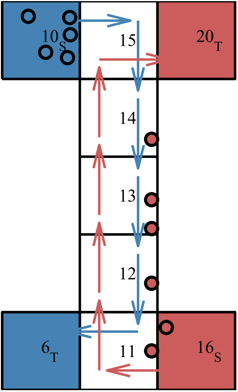
Moving entities over intersections requires some global coordination as illustrated by the following analogy. Consider the policy used to coordinate cars going in opposite directions over a one-lane bridge (see Figure 2), where there is a traffic signal on each side of the bridge. The algorithm chooses one traffic light, allowing some cars to safely travel over the bridge in one direction. After some time, the algorithm switches the lights (first turning green to red, and after the road is clear, turning red to green) allowing traffic to flow in the opposite direction. Then this process repeats.
⬇ 1 if for each 3 if then \lnlabel{pathif} : \lnlabel{pathset} 5 gossip the entity graph for each , : \lnlabel{pathgossip} 7 compute the set of color-shared cells \lnlabel{pathint} 9 if 11 graphs stabilized and i needs a lock for color c 13 if round \lnlabel{pathmutex} Initiate mutual exclusion algorithm between all 15 color-shared cells in using as input Eventually, a color is returned. 17 On return, if then detect if color-shared cells are empty 19 if round \lnlabel{pathempty} Initiate distributed snapshot algorithm to decide 21 if all color-shared cells are empty after previously being nonempty with entities of color c. 23 On return, if all cells are empty then Figure 9: function for . This function computes the color-shared cells—the cells in intersections—for each color, and then ensures liveness by giving a lock to only one color on each intersection.
Two parts of the previous example require global coordination and are included in the function. The first is how to chose the direction in which cars are allowed to travel—this is accomplished through the use of a mutual exclusion algorithm. The second is when to allow cars to travel in the opposite direction—this is accomplished by determining when the intersection is empty. We now describe this global coordination more formally.
For defining the locking algorithm, we first define intersections. For this we introduce the notion of an entity graph. Cell is said to be in the entity graph of some color at state if one of the following conditions hold: (a) is , (b) in state , has entities of color , or (c) in state , is the neighbor closest to of a cell already in the entity graph. Formally, we define the color entity graph at state as , which is the following subgraph of the color routing graph . The vertices of are inductively defined as
The edges of are . For example, if all cells are empty, then is the sequence of cell identifiers defined by following the minimum distance (as defined by ) from the source to the target of color . That is, each is a simple path graph from source to target444Once cells have failed, this may stabilize to be a tree from any cell with entities of color to the target of color ..
Now we describe how the entity graph of each color is computed by each cell as the variable. If is on the entity graph of color , then we add and ’s variable for color to the entity graph (see Figure 9, lines LABEL:line:pathif and LABEL:line:pathset). Once the variables stabilize () and after an additional order of diameter rounds, the variable contains all the entity graphs since we gossip these graphs (line LABEL:line:pathgossip). That is, the graph formed by the variables stabilizes to equal , and contains the sequence of identifiers from any source or nonempty cell of color to the target of color ().
Next, the variable is computed to be the set of cell identifiers on the color entity graph that overlaps with any other colored entity graph (line LABEL:line:pathint). The cells involved in such non-empty intersections represent physical traffic intersections, and are called color-shared cells. These cells require coordinated locking for traffic flow to progress. Cell is in if and only if it will need a lock for color .
Formally, we define the color-shared cells, for a state , for any , as
In Figure 2, these are cells and . The variables stabilize to equal , at some state , for any color ().
Next, we need to determine the colors that will need to coordinate to schedule traffic through the color-shared cells. Then, a mutual exclusion algorithm is initiated between all cells for each disjoint set of cell colors in . Formally, we define the shared colors, for a state , for any , as
The variables stabilize at some state to equal , for any color .
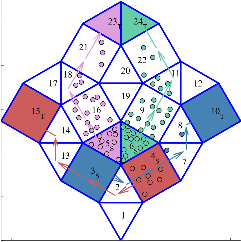
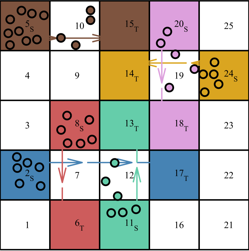
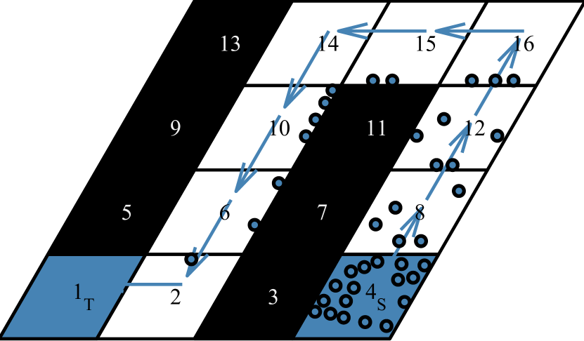
In general, up to colors could be involved in intersections, as well as all the smaller permutations. For instance, consider Figure 6 with colors at some state . Here, the blue and red entity graphs overlap, green and blue entity graphs overlap, but red and green do not, and independently, the purple and yellow entity graphs overlap (that is, not with blue, red, nor green), but no colors overlap with brown. Then is for equal to blue, red, or green, is for equal to yellow or purple, and is empty for equal to brown. Two mutual exclusion algorithms would be initiated, one with blue, red, and green as the input set of values, and another with yellow and purple as the input set. Upon these two instances terminating, one element of the first set, say , would be chosen and given a lock, and one element, say , of the second set would also be given a lock. The entities of these colors progress over the color-shared cells toward their intended targets. Finally, once the color-shared cells are empty again, and would each be removed from the respective input sets for fairness, and another mutual exclusion algorithm is initiated.
⬇ 1 if /\ then 3 5 if then choose from else 7 : 9 { \in : /\ \ne } \lnlabel{algo:type} ⬇ 11 if /\ then 13 15 if then choose from else 17 : 19 { \in : /\ \ne } \lnlabel{algo:type} 21 if then : choose from 23 let 25 if \A p \in : \lnlabel{signalSafe} /\ \lnlabel{signalOneColor} 27 /\ \lnlabel{signalLock} then \lnlabel{algo:lockout} 29 : if 1 then \lnlabel{algo:token1} 31 : choose from elseif 1 then \lnlabel{algo:token4} 33 : choose from else : 35 else : ; : \lnlabel{algo:tokenSame} Figure 10: function for . Cell signals fairly to some neighbor if it is safe for to move its entities toward .
The function (Figure 10) executes after . It is the key part of the protocol for maintaining safe entity separations, guaranteeing each cell has entities of only a single color, and ensuring progress of entities to the target. Roughly, each cell implements this through the following policies: (a) only accept entities from a neighbor when it is safe to do so, (b) only accept entities with the same color as the entities currently on the cell (or an arbitrary color if the cell is empty), (c) if a lock is needed, then only let entities move if it is acquired, and (d) ensure fairness by providing opportunities infinitely often for each nonempty neighbor to make progress.
First computes a temporary variable , which is the set of colors for any neighbor that has entities of some color, with the corresponding variable set to cell . Next, cell picks a color from this set if it is empty, or the color of its own entities if it is nonempty, and will attempt to allow some cell with this chosen color to move toward itself. Then, cell sets to be the subset of for which has been set to and is nonempty. If is , then it is set to some arbitrary value in , but it continues to be if is empty. Otherwise, for some neighbor of with nonempty . This is accomplished through the conditional in line LABEL:line:algo:gap as a step in guaranteeing fairness.
It is then checked if there is any entity with center in the safety region of on the side corresponding to . If there is such an entity, then is set to , which blocks the neighboring cell with identifier from moving its entities in the direction of , thus preventing entity transfers and ensuring safety. Otherwise, if there is no entity with center in the safety region on side , then is set to to allow to move its entities toward . Subsequently, is updated to a value in that is different from its previous value, if that is possible according to the rules just described (lines LABEL:line:algo:token1–LABEL:line:algo:token4).
Finally, the function (Figure 11) models the physical movement of all the entities on cell over a given round. For cell , let be , where is (which may be if cell has no entities). Every entity in moves in the direction of if and only if is set to . The direction followed from cell to is , which is any vector satisfying Assumption 1. For example, for a square (or rectangular) cell , one choice for is the unit vector orthogonal to and pointing into . In the case of an equilateral triangular cell , one choice for is also any orthogonal vector pointing into .
The movement toward cell may lead to some entities crossing the boundary of into , in which case, they are removed from . If is not the target matching the transferred entities’ color, then the removed entities are added to . In this case (line LABEL:line:algo:reset), any transferred entity is placed so that touches a single point of (is tangent to) , the shared side of cells and , and lies on the inner side of the transfer region of cell on side . Resetting entity positions is a conservative approximation to the actual physical movement of entities. If is the target matching the transferred entities’ color, then the removed entities are not added to any cell and thus no longer exist in .
⬇ 1 let c let 3 if /\ then for each p 5 : + \lnlabel{algo:movement} if \lnlabel{algo:gap} then 7 : {p} if \lnlabel{algo:movementTB} then 9 : \cup {p} \lnlabel{algo:reset} point on shared side along movement vector 11 : inner transfer region along orthogonal line 13 : %\taylor{we add the normal vector beyond the side length, need temp variable} 15 % Figure 11: function for . If has received a signal to move from , it updates the positions of all entities on it to move in ’s direction, which may lead to some entities transferring from cell to .
The source cells , in addition to the above, add a finite number of entities in each round to , such that the addition of these entities does not violate the minimum gap between entities at . In the remainder of the paper, we will analyze to show that in spite of failures, it maintains safety and liveness properties to be introduced in the next section.
4 Analysis of Distributed Traffic Control
In this section, we present an analysis of the safety and liveness properties of . Roughly, the safety property requires that there is a minimum gap between entities on any cell, and the liveness property requires that all entities that reside on cells with feasible paths to the corresponding target eventually reach that target.
4.1 Safety and Collision Avoidance
A state is safe if, for every cell, the boundaries of all entities in the cell are separated by a distance of . For any state of , we define:
This definition allows entities in different cells to be closer than apart, but their centers will be spaced by at least . We proceed by proving some preliminary properties of that will be used for proving is an invariant.
The first property asserts that entities’ cannot come close enough to the sides of cells to reside on multiple cells. This is because any entity whose boundary touches the side of a cell is transferred to the neighboring cell on that side (if one exists), and then the entity’s position is reset to be completely within the new cell. Assumption 2 restricts the allowed partitions to ensure entity transfers are well-defined. For instance, some of the cells in the snub square tiling in Figure 4 do not satisfy Assumption 2. Consider an entity transfer from cell to cell . There is no constant vector connecting the transfer regions of cell to those of cell . This is because the side length of the transfer region of the triangular cell is shorter than the side length of the transfer region of the square cell . However, in a transfer from cell to cell or vice-versa, the side lengths are the same. We also note that the assumption is only necessary for entity transfers from a cell with a longer transfer side length to a neighboring cell with smaller corresponding transfer side length. For example, a transfer from cell to cell is feasible.
Under Assumption 2, we have the following invariant, which states that the -ball around each entity in a cell is completely contained within the cell.
Invariant 1.
In any reachable state , , , .
The next invariant states that cells’ sets are disjoint. This is immediate from the function since entities are only added to one cell’s upon being removed from a different cell’s .
Invariant 2.
In any reachable state , for any , if , then .
The following invariant states that cells contain entities of a single color in spite of failures. This follows from the routine in Figure 10, where line LABEL:line:signalOneColor requires that if some neighbor is attempting to move entities toward cell , then the color of is either or equal to the color of .
Invariant 3.
In any reachable state , for all , for all , .
Next, we define a predicate that states that if is set to the identifier of some neighbor , then there is a large enough area from the common side between and where no entities reside in . Recall that is the line segment shared between neighboring cells and . For a state , , , if , then the following holds:
is not an invariant property because once entities move the property may be violated. However, for proving safety, all that needs to be established is that at the point of computation of the variable this property holds. The next key lemma states this.
Lemma 4.
For all reachable states , where is the state obtained by applying the , , and functions to .
Proof.
Fix a reachable state , an , and an such that . Let be the state obtained by applying the function to , be the state obtained by applying the function to , and be the state obtained by applying the function to .
First, observe that both and hold. This is because the and functions do not change any of the variables involved in the definition of . Next, we show that implies . If then the statement holds vacuously. Otherwise, , then since (a) holds, and (b) Figure 10, line LABEL:line:algo:gap is satisfied, we have that . ∎
The following lemma asserts that if there is a cycle of length two formed by the variables—which could occur due to failures—then entity transfers cannot occur between the involved cells in that round.
Lemma 5.
Let be any reachable state and be a state that is reached from after a single transition (round). If and , then and .
Proof.
No entities enter either or from any other or since and . It remains to be established that such that where or vice-versa. Suppose such a transfer occurs. For the transfer to have occurred, must be such that by Figure 11, line LABEL:line:algo:movement. But for to be satisfied, it must have been the case that by Figure 10, line LABEL:line:algo:gap and since , a contradiction is reached. ∎
Using the previous results, we now prove that preserves safety even when some cells fail.
Theorem 1.
In any reachable state of , .
Proof.
The proof is by standard induction over the length of any execution of . The base case is satisfied by the assumption that initial states satisfy . For the inductive step, consider any reachable states , and an action such that . Fix and assuming , we show that . If , then since no entities move.
For , there are two cases to consider by Invariant 2. First, , that is, no new entities were added to , but some may have transfered off . There are two sub-cases: if , then all entities in move identically and the spacing between two distinct entities , is unchanged. Let where by Invariant 3. That is, , such that and and where , (Figure 11, line LABEL:line:algo:movement). It follows by the inductive hypothesis that . The second sub-case arises if , then is either vacuously satisfied or it is satisfied by the same argument just stated.
The second case is when , that is, there was at least one entity transfered to . Consider any such transferred entity where . There are two sub-cases. The first sub-case is when was added to because is a source, that is, . In this case, the specification of the source cells states that the entity was added to without violating , and the proof is complete. Otherwise, was added to by some neighbor , so but , and but . From line LABEL:line:algo:reset of Figure 11, we have that that . The fact that transferred from in to in implies that and —these are necessary conditions for the transfer by Figure 10, line LABEL:line:signalSafe. Thus, applying the predicate at state and by Lemma 4, it follows that for every , . It must now be established that if is transfered to , then every , where satisfies , which means that any entity already on did not move toward the transfered entity that is now on . This follows by application of Lemma 5, which states that if entities on adjacent cells move towards one another simultaneously, then a transfer of entities cannot occur. This implies that the discs of all entities in are farther than of the borders of any transfered entity , implying . Finally, since was chosen arbitrarily, . ∎
Theorem 1 shows that is safe in spite of failures.
4.2 Stabilization of Spanning Routing Trees
Next, we show under some additional assumptions, that once new failures cease to occur, recovers to a state where each non-faulty cell with a feasible path to its target computes a route toward it. This route stabilization is then used in showing that any entity on a non-faulty cell with a feasible path to its target makes progress toward it. Our analysis relies on the following assumptions on cell failures and the placement of new entities on source cells. The first assumption states that no target cells fail, and is reasonable and necessary because if any target cell did fail, entities of that color obviously cannot make progress.
Assumption 3.
No target cells may fail.
The next assumption ensures source cells place entities fairly so that they may not perpetually prevent any neighboring cell or any color-shared cell from making progress. The assumption is needed because it provides a specification of how the source cells behave, which has not been done so far. The assumption is reasonable because it essentially says that traffic is not produced perpetually without any break.
Assumption 4.
(Fairness): Source cells place new entities without perpetually blocking either (i) any of their nonempty non-faulty neighbors, or (ii) any cell , where is the color of source .
Formally, the first fairness condition states, for any execution of , for any color , for any source cell , if there exists an , such that for every state in after a certain round, , then eventually becomes equal to in some round of . The second fairness condition states, for any execution of , for any state , for any color , for any source cell , if there exists an such that , and for every state in after a certain round, if cell is nonempty, then eventually becomes equal to in some round of , where is a neighbor of . Such conditions can be ensured if we suppose some oracle placing entities on source cells follows the same round-robin like scheme defined in the subroutine in Figure 10. Scenarios where each of these cases can arise are illustrated in Figure 6.
A fault-free execution fragment be a sequence of states starting from and along which no transitions occur. That is, a fault-free execution fragment is an execution fragment with no new failure actions, although there may be existing failures at the first state of , so need not be empty. Throughout the remainder of this section, we will consider fault-free executions that satisfy Assumptions 3 and 4.
Lemma 6.
Consider any reachable state of , any color , and any . Let . Any fault-free execution fragment starting from stabilizes within rounds to a set of states with all elements satisfying:
Proof.
Fix an arbitrary state , a fault-free execution fragment starting from , a color , and . We have to show that (a) the set of states is closed under transitions and (b) after rounds, the execution fragment enters .
First, by induction on we show that is stable. Consider any state and a state that is obtained by applying an transition to . We have to show that . For the base case, , so and . From lines LABEL:line:algo:distmin and LABEL:line:algo:nextmin of the function in Figure 8, and that there is a unique for each color , it follows that remains and remains . For the inductive step, the inductive hypothesis is, for any given , if for any , and , for some with , then
Now consider such that . In order to show that is closed, we have to assume that and , and show that the same holds for . Since , does not have a neighbor with target distance smaller than . The required result follows from applying the inductive hypothesis to and from lines LABEL:line:algo:distmin and LABEL:line:algo:nextmin of Figure 8.
Second, we have to show that starting from , enters within rounds. Once again, this is established by induction on , which is . Consider any state such that . The base case only includes the target distances satisfying and follows by instantiating . For the inductive case, assume for the inductive hypothesis that at some state , and such that , where is the minimum identifier among all such cells (since we used cell identifiers to break ties). Observe that there is one such by the definition of . Then at state , by the inductive hypothesis and lines LABEL:line:algo:distmin and LABEL:line:algo:nextmin of Figure 8, . ∎
The following corollary of Lemma 6 states that, after new failures cease occurring, for all target-connected cells, the graph induced by the variables stabilizes to the color routing graph, , within at most the diameter of the communication graph number of rounds, which is bounded by .
Corollary 7.
Consider any execution of with an arbitrary but finite sequence of transitions. For any state at least rounds after the last transition, for any , every cell target-connected to color has equal to the identifier of the next cell along such a route.
The following corollary of Lemma 6 and states that within rounds after routes stabilize, for each color , the identifiers in the variables equal the vertices of the color entity graph . The result follows since routes stabilize and that is a function of and variables only, and that variables are gossiped in Figure 9, line LABEL:line:pathgossip.
Corollary 8.
Consider any execution of with an arbitrary but finite sequence of transitions. For any state at least rounds after the last transition, for every , every cell target-connected to color has .
The next corollary of Lemma 6 states that eventually the values of the variables equal the set of color-shared cells for any cell and color . This is important because the mutual exclusion algorithm is initiated between the cells in (Figure 9, line LABEL:line:pathmutex).
Corollary 9.
Consider any execution of with an arbitrary but finite sequence of transitions. For any state at least rounds after the last transition, for every , every cell target-connected to color has .
4.3 Scheduling Entities through Color-Shared Cells
In this section, we show that there is at most a single color on the set of color-shared cells if there are no failures. We then show that any cell that requests a lock eventually gets one, under an additional assumption that failures do not cause entities of more than one color to reside on the set of color-shared cells. Because failures cause the routing graphs and entity graphs to change, the color-shared cells that could previously be scheduled may now be deadlocked. Additionally, because we separately lock each disjoint set of color-shared cells to allow entities of some color to flow toward their target, it could be the case that the intermediate states between when the failure occurred and when routes have stabilized allowed entities to move in such a way that deadlocks the system. Such deadlocks could be avoided if a centralized coordinator informs every non-faulty cell to disable their signals when a failure is detected. The assumption states that with failures, the color-shared cells either all have the same-colored entities, or have no entities (and combinations thereof).
Assumption 5.
Feasibility of Locking after Failures: For any reachable state , for any color , consider the color-shared cells . For all distinct cells either or .
The next lemma states that without failures, there are entities of at most a single color on the set of color-shared cells. The result is not an invariant because failures may cause the set of color-shared cells to change, resulting in deadlocks, which is why we need Assumption 5. By Invariant 3, we know that there are entities of at most a single color in each cell, so the following invariant is stated in terms of the color of each cell. We emphasize that Assumption 5 is unnecessary if there are no failures, as the algorithm ensures there are entities of at most a single color on the color-shared cells by the following lemma.
Lemma 10.
If there are no failures, for any reachable state , for any , for any , if , then for all , we have .
Proof.
The proof is showing an inductive invariant, supposing no failures occur. For the initial state, all cells are empty, so we have for any . For the inductive step, we are only considering actions by assumption. In the pre-state, we have and , we have . Fix some and some . For any subsequent state , if , the result follows vacuously. If , we must show that , so fix some . If , the result follows, since by the inductive hypothesis, . If , the condition in (Figure 10, line LABEL:line:signalLock) cannot be satisfied since . Thus, no cell with entities of color could move toward any cell in , and we have . ∎
The next lemma states that without failures, or with “nice” failures as described by Assumption 5, that any cell requesting a lock of some color will eventually get it, and thus it may move entities onto the color-shared cells.
Lemma 11.
For any reachable state satisfying Assumption 5, for any , for any , if and all cells in are empty, then eventually a state is reached where .
Proof.
By correctness of the mutual exclusion algorithm, eventually a color is returned and (Figure 9, line LABEL:line:pathmutex). If , then the result follows. If , by Lemma 10 and Assumption 5, we know that no other color aside from has entities on any cell . The next time the mutual exclusion algorithm is initiated, is excluded from the input set to the mutual exclusion algorithm (Figure 9, line LABEL:line:pathempty), and by repeated argument, eventually . ∎
4.4 Progress of Entities towards their Targets
Using the results from the previous sections, we show that once new failures cease occurring, for every color , every entity of color on a cell that is target-connected eventually gets to the target of color . The result (Theorem 2) uses two lemmas which establish that, along every infinite execution with a finite number of failures, every nonempty target-connected cell gets permission to move infinitely often (Lemma 13), and a permission to move allows the entities on a cell to make progress towards the target (Lemma 12).
For the remainder of this section, we fix an arbitrary infinite execution of with a finite number of failures, satisfying Assumption 5. Let be any state of at least rounds after the last failure, and be the infinite failure-free execution fragment , , of starting from . For any , observe that the number of target-connected cells remains constant starting from for the remainder of the execution. That is, , so we fix .
Lemma 12.
For any , for any , for some , if , , and , for any entity , let the distance function be defined by the lexicographically ordered tuple
where is the point on the shared side defined by the line passing through with direction . Then, .
Proof.
The first case is when no entity transfers from to in the round: if such that , then . In this case, the result follows since a velocity is applied towards cell by in Figure 11, line LABEL:line:algo:movement. The second case is when some entity transfers from to , so such that . In this case, we have , since the distance between and is smaller than the distance between and since routes have stabilized by Lemma 6. In either case, , so entity is closer to the appropriate target. ∎
The following lemma states that all cells with a path to the target receive a signal to move infinitely often, so Lemma 12 applies infinitely often.
Lemma 13.
For any , consider any , such that for all , if , then such that .
Proof.
Fix some . Since , there exists such that for all , . We prove the lemma by inducting on . The base case is . Fix and instantiate . By Lemma 6, for any , for all non-faulty , since . For all , if , then changes to a different neighbor with entities every round. It is thus the case that and since always, exactly one neighbor satisfies the conditional of Figure 10, line LABEL:line:algo:gap in any round, then within rounds, .
For the inductive case, let be the step in after which all non-faulty have by Lemma 6. Also by Lemma 6, such that , implying that after , since and . By the inductive hypothesis, infinitely often. If , then entity initialization does not prevent from being satisfied infinitely often by the second assumption introduced in Subsection 4.2. It remains to be established that infinitely often. Let where .
In any of the following cases, if and all cells are empty, then by Lemma 11, eventually . If , then since the inductive hypothesis satisfies infinitely often, then Lemma 12 applies infinitely often, and thus infinitely often, finally implying that infinitely often.
If , there are two sub-cases. The first sub-case is when no entity enters from some , which follows by the same reasoning used in the case. The second sub-case is when a entity enters from , in which case it must be established that infinitely often. This follows since if where and is the round at which an entity entered from , and the appropriate case of Lemma 4 is not satisfied, then and by Figure 10, line LABEL:line:algo:tokenSame. This implies that no more entities enter from either cell satisfying . Thus infinitely often follows by the same reasoning case. ∎
The final theorem establishes that entities on any cell in eventually reach the target in .
Theorem 2.
For any , consider any , , , such that .
Proof.
Fix , , a round and . Let which is finite. By Lemma 6, at every round after for any , the sequence of identifiers , , , forms a fixed path to . Applying Lemma 13 to shows that there exists such that . Now applying Lemma 12 to establishes movement of towards , which is also . Lemma 13 further establishes that this occurs infinitely often, thus there is a round such that gets transferred to . ∎
By an induction on the sequence of identifiers in the path , it follows that entities on any cell in eventually get consumed by the target.
Summary of Results
In this section, we establish several invariant properties culminating in proving safety of the system, which meant that entities never collide, in spite of failures. Next, we proved that the routing algorithm used to construct paths to the destinations is self-stabilizing in spite of arbitrary crash failures. We next showed under an assumption that failures do not introduce deadlock scenarios that the locking algorithm allows multi-color flows to mutual exclusively take control of intersections (color-shared cells). Finally, under a fairness assumption, we established the main progress property through two results, that any cell gets permission to move infinitely often, and that any cell with a permission to move decreases the distance of any entities on it from its destination.
5 Simulation Experiments
We have performed several simulation studies of the algorithm for evaluating its throughput performance. In this section, we discuss the main findings with illustrative examples taken from the simulation results. We implemented the simulator in Matlab, and all the partition figures displayed in the paper are created using it.
Let the -round throughput of be the total number of entities arriving at the target over rounds, divided by . We define the average throughput (henceforth throughput) as the limit of -round throughput for large . All simulations start at a state where all cells are empty and subsequently entities are added to the source cells.
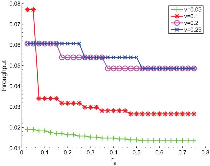
Single-color throughput without failures as a function of , ,
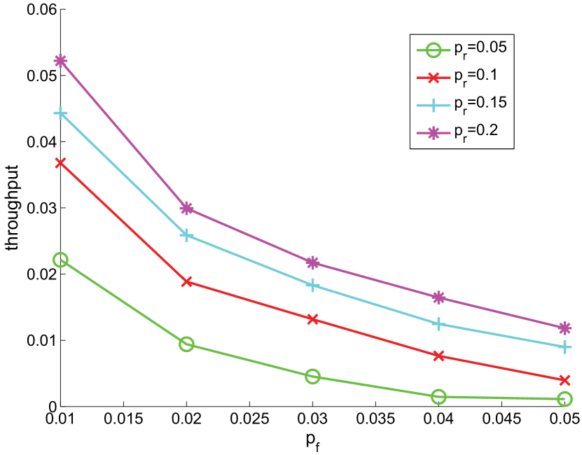
Rough calculations show that throughput should be proportional to cell velocity , and inversely proportional to safety distance and entity radius . Figure 13 shows throughput versus for several choices of for an unit square tessellation instance of with a single entity color. The parameters are set to and . The entities move along a line path where the source is the bottom left corner cell and the target is the top left corner cell. For the most part, the inverse relationship with holds as expected: all other factors remaining the same, a lower velocity makes each entity take longer to move away from the boundary, which causes the predecessor cell to be blocked more frequently, and thus fewer entities reach from any element of in the same number of rounds. In cases with low velocity (for example ) and for very small , however, the throughput can actually be greater than that at a slightly higher velocity. We conjecture that this somewhat surprising effect appears because at very small safety spacing, the potential for safety violation is higher with faster speeds, and therefore there are many more blocked cells per round. We also observe that the throughput saturates at a certain value of (). This situation arises when there is roughly only one entity in each cell.
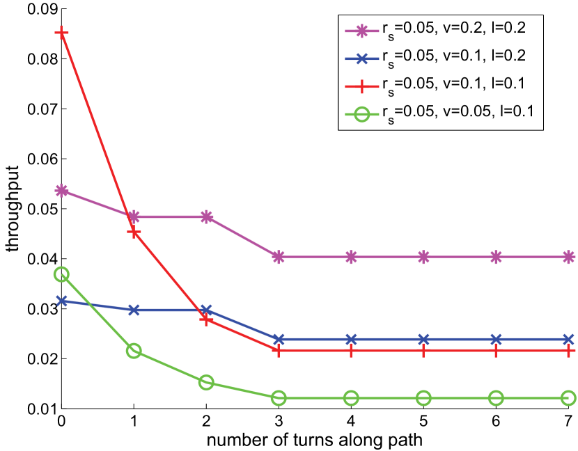
Single-color throughput without failures as a function of the path
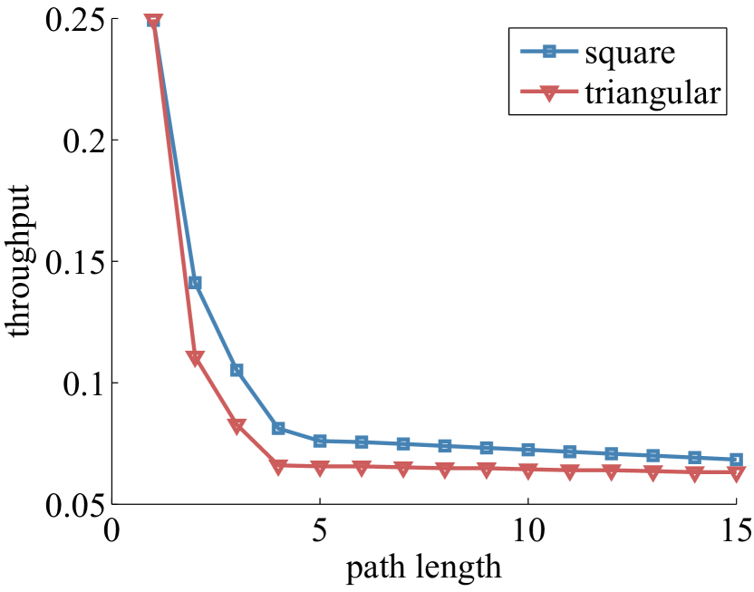
For a sufficiently large number of rounds , throughput is independent of the length of the path. This of course varies based on the particular path and instance of considered, but all other variables fixed, this relationship is observed. More interesting however, is the relationship between throughput and path complexity, measured in the number of turns along a path. Figure 13 shows throughput versus the number of turns along paths of length . This illustrates that throughput decreases as the number of turns increases, up to a point at which the decrease in throughput saturates. This saturation is due to signaling and indicates that there is only one entity per cell.
Single-color throughput under failure and recovery of cells
Finally, we considered a random failure and recovery model in which at each round each non-faulty cell fails with some probability and each faulty cell recovers with some probability [33]. A recovery sets and in the case of also resets , so that eventually will correct and for any . Intuitively, we expect that throughput will decrease as increases and increase as increases. Figure 15 demonstrates this result for and . There is a diminishing return on increasing for a fixed , in that for a fixed increasing results in smaller throughput gains.
Multi-color throughput as a function of the number of intersecting cells
Now we discuss the influence of multi-color throughput. In the case where the paths between different sources and targets do not overlap, all the results from the single-color simulation results apply. In the case where the paths do overlap, the mutual exclusion algorithm runs to ensure no deadlocks occur. This additional control logic will have an influence on the throughput. For the multi-color cases, we consider the summed throughput, which is the sum of the throughputs for each color.
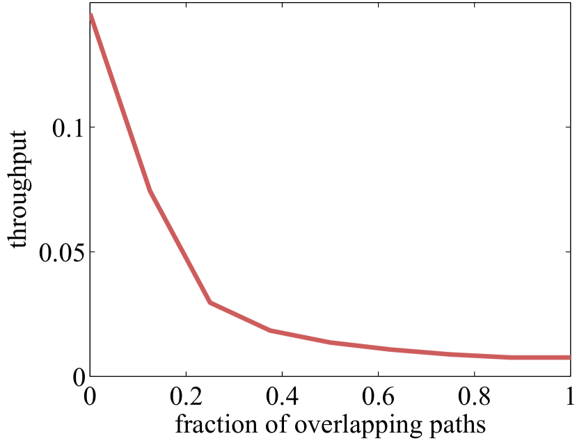
Figure 17 shows the roughly exponential decrease in throughput as the fraction of overlapping paths increases for two colors with path length and no turns. The fraction of overlapping paths is defined as the number of vertices in the color-shared cells . As the fraction increases, the paths lie completely on top of one another, so in this case with path length , we have no overlap, cell overlap, etc.
Multi-color throughput as a function of the number of intersecting colors
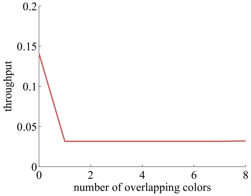
Intersections (that is, having at least one color-shared cell) have a fixed cost on throughput. Specifically, the summed throughput of there being two overlapping colors on a cell is the same as the summed throughput of three or more. Figure 17 shows this fixed decrease in throughput as the number of overlapping colors increases for a fixed path of length with color-shared cells, where the decrease in throughput from having no overlaps to having one color overlapping is about times. Once there are two colors, all additional colors do not decrease throughput. This observation agrees with intuition—the decrease in throughput due to an intersection is independent of the number of destinations for the entities that must pass through that intersection.
6 Related Work
There is a large amount of work on traffic control in transportation systems (see, e.g., [4, 34]) and robotics (see, e.g., [35]). We briefly summarize some of the more related work, but highlight that we are presenting a formal model of an example of such systems. Distributed air and automotive traffic control have been studied in many contexts. Human-factors issues are considered in [36, 37] to ensure collision avoidance between the coordination of numerous pilots and a supervisory controller modeling the semi-centralized air traffic control components. The Small Aircraft Transportation Protocol (SATS) is semi-distributed air traffic control protocol designed for small airports without radar, so pilots and their aircraft coordinate among themselves to land after being assigned a landing sequence order by an automated system at the airport [16]. SATS has been formally modeled and analyzed using a combination of model checking and automated theorem proving [38]. SATS and this paper share an abstraction: the physical environment is a priori partitioned into a set of regions of interest, and properties about the whole system are proved using compositional analysis. Safe conflict resolution maneuvers for distributed air traffic control are designed in [39]. A formal model of the traffic collision avoidance system (TCAS) is developed and analyzed for safety in [40]. TCAS is a system deployed on aircraft that alerts pilots when other aircraft are in close proximity and guides them along safe trajectories.
A distributed algorithm (executed by entities, vehicles in this case) for controlling automotive intersections without any stop signs is presented in [18]. Some methods for ensuring liveness for automotive intersections are presented in [41]. A method to detect the mode of a hybrid system control model of an autonomous vehicle in intersections is developed in [42], and is used to reduce conservatism of the maximally controlled invariant set (the set of collision-free controls). Efficient distributed intersection control algorithms are developed in [43]. There is a large amount of work on flocking [44] and platooning [45, 46, 47, 48]. Only a few works consider failures in such systems, like the arbitrary failures considered in [49, 50], the actuator failures considered in [48], or in synchronization of swarm robot systems in [51].
Distributed robot coordination on discrete abstractions like [52, 23, 53, 54, 55, 56, 57] can be viewed as traffic control. For instance, [23] establishes a formal connection between the continuous and the discrete parts of these protocols, and also presents a self-stabilizing algorithm with similar analysis to the analysis in this paper. These works also decompose the continuous problem into a discrete abstraction by partitioning the environment, but all these works allow at most a single entity (robot) in each partition, while our framework allows numerous entities in each partition. If several entities are to visit some destination in [53, 56, 57], like our targets here, that destination is represented as the union of a set of partitions and each entity must reside in one of these partitions.
The Kiva Systems robotic warehouse [52] is a robotic traffic control system on square partitions, and can be described in our framework by allowing a single entity per cell. In these warehouse systems, there is a central coordinator scheduling tasks, but the robots are responsible for path planning using an A∗-like search algorithm [52]. However, several deadlock scenarios are identified when performing such path planning [54]. The Adaptive Highways Algorithm presented in [54] for scheduling entities relies on using the tentative trajectories of other robots collected by the central controller. Deadlocks are also observed in other distributed robotics path-planning algorithms on discrete partitions in [58]. Deadlock scenarios can also arise without a discrete abstraction, such as in the doorways considered in [59], the path formation algorithms of [60], or the warehouse automation system of [61].
7 Discussion
In this section, we discuss some ways to generalize assumptions used in the paper and some alternative methods. In this paper, we presented a distributed traffic control algorithm for the partitioned plane, which moves entities without collision to their destinations, in spite of failures. While our algorithm is presented for two-dimensional partitions, an extension to some three-dimensional partitions (e.g., cubes and tetrahedra) follows in an obvious way. An extension to the more general case where there are multiple sources and multiple targets of each color—and entities of each color move toward the nearest target of that color—is straightforward, but complicates notation.
Self-Stabilizing Mutual Exclusion and Distributed Snapshot Algorithms
There are a variety of mutual exclusion algorithms that could be used to determine locks (Figure 9, line LABEL:line:pathmutex). For this paper, we require the overall system to be stabilizing and therefore the locking algorithm itself should be stabilizing. To this end, any of the following algorithms could be adapted to our framework: the token circulation algorithm [65], mutual exclusion [66], group mutual exclusion [67], snap-stabilizing propagation of information with feedback (PIF) algorithm [68], or -out-of- mutual exclusion [69]. A self-stabilizing distributed snapshot algorithm (see [27, Ch. 5]) can be used to determine if all color-shared cells are empty, after having had some entity of color (Figure 9, line LABEL:line:pathempty). If all cells are empty, then another round of mutual exclusion commences, excluding color from the input set.
General Triangulations and Affine Dynamics
We assumed in Section 2 that the partitions satisfy several geometric assumptions for feasibility of entity transfers. We considered using vector fields generated by a discrete abstraction like those presented in [70, 71, 72, 73]. The affine vector fields generated on simplices in [70, 73] can be used to move an entity (with potentially nonholonomic or nonlinear dynamics) through any side of a cell in a triangulation (simplex) [70, 72] or rectangle [71]. However, it turns out that it is impossible to maintain our notion of safety for such vector fields without additional collision avoidance mechanisms implemented on each entity. This is due to a simple geometric observation—moving entities through a shorter side than the side they entered through may require the entities to come closer together. For example, if a cell in the triangulation has an obtuse angle, then the vector field generated by [70] flowing from the longest edge to the shortest edge has negative divergence. Furthermore, a vector field having negative divergence implies the flow corresponding to any two distinct points starting in that field come closer together, hence safety cannot be maintained. The distributed problems using these discrete abstractions [53, 56, 57] avoid this by requiring at most one entity in any (triangular) partition at a time.
We also mention a simple condition to ensure that triangulations have the required geometric partition properties (Assumptions 1 and 2). If all the triangles in the triangulation are non-obtuse, then the triangulation satisfies these assumptions. We also note that restricting allowable triangulations of an environment to ones without obtuse angles is not restrictive, since any polygon can be efficiently partitioned into a triangulation with non-obtuse [74, 75] or acute [76] angles.
Insufficiency of Disjoint Paths
Finding disjoint paths, such as by using the algorithms from [77, 78, 79, 80], could be another approach to solving the multi-color problem, but the locking mechanism used here solves a more general problem. Even without failures, there are many environments and choices of sources and targets for which there are no disjoint paths between sources and targets. One such environment is shown in Figure 4, where for two distinct colors and , the paths between the respective sources and targets necessarily overlap, so an algorithm for finding disjoint paths cannot be used as there are no disjoint paths between sources and targets. However, there are disjoint paths in some cases, so no scheduling would be necessary if these are found, but our routing algorithm does not necessarily find these, as the disjoint paths may not be shortest distance. A self-stabilizing algorithm for finding disjoint paths on planar graphs would be an enhancement to our algorithm, as it would increase throughput in the case that paths need not overlap.
Back-Pressure and Wormhole Routing
Back-pressure routing [81, 82] is an algorithm for dynamically routing traffic over an underlying graph using congestion gradients. If we view the color of each entity as its intended address and consider this problem from the perspective of queuing theory, one might think back-pressure routing could provide a throughput-optimal solution for the problem. However, our physical motion model is incompatible with back-pressure routing. For a given cell, our model does not allow arbitrary choice of the next neighbor for each entity on that cell. In particular, when one cell moves its entities toward a neighboring cell, all entities sufficiently near the shared side between the two neighbors would transfer.
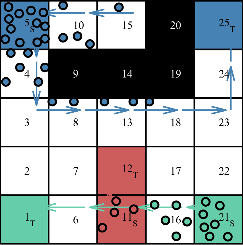
Wormhole routing [83] is a flow control policy over a fixed underlying graph for determining when packets move to the node on the graph. Addresses in wormhole routing are very short and come at the beginning of a packet, so a packet can be subdivided into pieces or flits and begin being forwarded after the address is received, yielding a snake-like sequence of flits in transfer. One could also view the sequence of entities on a path toward the appropriately-colored target (see Figure 19) sequence of flits flowing to a destination in wormhole routing. While similar deadlock scenarios can arise in our system and wormhole routing, wormhole routing is incompatible with our system due to the motion model just like back-pressure routing.
8 Conclusion
We presented a self-stabilizing distributed traffic control protocol for the partitioned plane, where each partition controls the motion of all entities within that partition. The algorithm guarantees separation between entities in the face of crash failures of the software controlling a partition. Once new failures cease occurring, it guarantees progress of all entities that are neither isolated by (a) failed partitions, nor (b) cells with entities of other colors that become deadlocked due to failures, to the respective targets. Through simulations, we presented estimates of throughput as a function of velocity, minimum separation, single-target path complexity, failure-recovery rates, and multi-target path complexity.
It would be interesting to develop strategies allowing entities of different colors on a single cell. Our strategy of preventing entities of different colors from residing on a single cell simplified some analysis, but it also complicated some analysis, by making it harder to prove progress because deadlock scenarios may frequently arise. It would be interesting to develop algorithms allowing mixing and sorting of colors using different types of motion coupling. It would also be interesting to design algorithms that can allow relaxing the assumption on what failures may occur to ensure liveness. We believe this would require a more complex routing algorithm to temporarily move entities of some colors off the color shared cells, thus allowing some other color on the color shared cells to make progress.
9 Acknowledgments
The authors thank Zhongdong Zhu for helping develop the current version of the simulator, Karthik Manamcheri for helping develop an earlier version of the simulator, and Nitin Vaidya for helpful feedback. We also thank the anonymous reviewers who helped improve the earlier version of this paper.
References
- [1] D. Helbing, M. Treiber, Jams, waves, and clusters, Science
- [2] B. S. Kerner, Experimental features of self-organization in traffic flow, Phys. Rev. Lett.
- [3] C. Daganzo, M. Cassidy, R. Bertini, Possible explanations of phase transitions in highway traffic, Transportation Research A
- [4] M. Nolan, Fundamentals of air traffic control,
- [5] F. Borgonovo, L. Campelli, M. Cesana, L. Coletti, Mac for ad hoc inter-vehicle network: services and performance, in: IEEE Vehicular Technology Conf., Vol. 5, 2003,
- [6] M. Karpiriski, A. Senart, V. Cahill, Sensor networks for smart roads, in: Pervasive Computing and Communications Workshops, 2006. PerCom Workshops 2006. Fourth Annual IEEE International Conference on, 2006,
- [7] S. S. Manvi, M. S. Kakkasageri, J. Pitt, Multiagent based information dissemination in vehicular ad hoc networks, Mob. Inf. Syst.
- [8] S. R. Azimi, G. Bhatia, R. R. Rajkumar, P. Mudalige, Vehicular networks for collision avoidance at intersections, SAE International Journal of Passenger Cars - Mechanical Systems
- [9] S. Thrun, M. Montemerlo, H. Dahlkamp, D. Stavens, A. Aron, J. Diebel, P. Fong, J. Gale, M. Halpenny, G. Hoffmann, K. Lau, C. Oakley, M. Palatucci, V. Pratt, P. Stang, S. Strohband, C. Dupont, L.-E. Jendrossek, C. Koelen, C. Markey, C. Rummel, J. van Niekerk, E. Jensen, P. Alessandrini, G. Bradski, B. Davies, S. Ettinger, A. Kaehler, A. Nefian, P. Mahoney, Stanley: The Robot That Won the DARPA Grand Challenge, in: M. Buehler, K. Iagnemma, S. Singh (Eds.), The 2005 DARPA Grand Challenge, Vol. 36 of Springer Tracts in Advanced Robotics, Springer Berlin / Heidelberg, 2007,
- [10] C. Urmson, J. Anhalt, D. Bagnell, C. Baker, R. Bittner, M. N. Clark, J. Dolan, D. Duggins, T. Galatali, C. Geyer, M. Gittleman, S. Harbaugh, M. Hebert, T. M. Howard, S. Kolski, A. Kelly, M. Likhachev, M. McNaughton, N. Miller, K. Peterson, B. Pilnick, R. Rajkumar, P. Rybski, B. Salesky, Y.-W. Seo, S. Singh, J. Snider, A. Stentz, W. R. Whittaker, Z. Wolkowicki, J. Ziglar, H. Bae, T. Brown, D. Demitrish, B. Litkouhi, J. Nickolaou, V. Sadekar, W. Zhang, J. Struble, M. Taylor, M. Darms, D. Ferguson, Autonomous driving in urban environments: Boss and the urban challenge, Journal of Field Robotics
- [11] X. Yang, L. Liu, N. Vaidya, F. Zhao, A vehicle-to-vehicle communication protocol for cooperative collision warning, in: Mobile and Ubiquitous Systems: Networking and Services. MOBIQUITOUS. The First Annual International Conference on, 2004,
- [12] J. Misener, R. Sengupta, H. Krishnan, Cooperative collision warning: Enabling crash avoidance with wireless technology, in: 12th World Congress on Intelligent Transportation Systems, 2005,
- [13] B. Hoh, M. Gruteser, R. Herring, J. Ban, D. Work, J.-C. Herrera, A. M. Bayen, M. Annavaram, Q. Jacobson, Virtual trip lines for distributed privacy-preserving traffic monitoring, in: MobiSys ’08: Proceeding of the 6th International Conference on Mobile Systems, Applications, and Services, ACM, New York, NY, USA, 2008,
- [14] A. Girard, J. de Sousa, J. Misener, J. Hedrick, A control architecture for integrated cooperative cruise control and collision warning systems, in: Decision and Control. Proceedings of the 40th IEEE Conference on, Vol. 2, 2001,
- [15] M. Mamei, F. Zambonelli, L. Leonardi, Distributed motion coordination with co-fields: a case study in urban traffic management, in: Autonomous Decentralized Systems. ISADS. The Sixth International Symposium on, 2003,
- [16] T. S. Abbott, K. M. Jones, M. C. Consiglio, D. M. Williams, C. A. Adams, Small aircraft transportation system, higher volume operations concept: Normal operations, Tech. Rep. NASA/TM-2004-213022, NASA
- [17] M. Kelly, G. Di Marzo Serugendo, A decentralised car traffic control system simulation using local message propagation optimised with a genetic algorithm, in: S. Brueckner, S. Hassas, M. Jelasity, D. Yamins (Eds.), Engineering Self-Organising Systems, Vol. 4335 of Lecture Notes in Computer Science, Springer, 2007,
- [18] H. Kowshik, D. Caveney, P. R. Kumar, Safety and liveness in intelligent intersections, in: Hybrid Systems: Computation and Control (HSCC), 11th International Workshop, Vol. 4981 of LNCS, 2008,
- [19] K. Dresner, P. Stone, A multiagent approach to autonomous intersection management, Journal of Artificial Intelligence Research
- [20] P. Weiss, Stop-and-go science, Science News
-
[21]
Kornylak, Omniwheel
brochure
URL http://www.kornylak.com/images/pdf/omni-wheel.pdf. - [22] K. An, A. Trewyn, A. Gokhale, S. Sastry, Model-driven performance analysis of reconfigurable conveyor systems used in material handling applications, in: Cyber-Physical Systems (ICCPS), 2011 IEEE/ACM International Conference on, Vol. 2, IEEE, 2011,
- [23] S. Gilbert, N. Lynch, S. Mitra, T. Nolte, Self-stabilizing robot formations over unreliable networks, ACM Trans. Auton. Adapt. Syst.
- [24] S. Dolev, L. Lahiani, S. Gilbert, N. Lynch, T. Nolte, Virtual stationary automata for mobile networks, in: PODC ’05: Proceedings of the twenty-fourth annual ACM symposium on Principles of distributed computing, ACM, New York, NY, USA, 2005,
- [25] T. Nolte, N. Lynch, A virtual node-based tracking algorithm for mobile networks, in: Distributed Computing Systems, International Conference on (ICDCS), IEEE Computer Society, Los Alamitos, CA, USA, 2007,
- [26] A. Arora, M. Gouda, Closure and convergence: A foundation of fault-tolerant computing, IEEE Trans. Softw. Eng.
- [27] S. Dolev, Self-stabilization,
- [28] S. M. Loos, A. Platzer, L. Nistor, Adaptive cruise control: Hybrid, distributed, and now formally verified, in: M. Butler, W. Schulte (Eds.), Formal Methods, LNCS,
- [29] A. Platzer, Quantified differential invariants, in: Proc. of the 14th ACM Intl. Conf. on Hybrid Systems: Computation and Control, ACM, 2011,
- [30] T. T. Johnson, S. Mitra, Parameterized verification of distributed cyber-physical systems: An aircraft landing protocol case study, in: ACM/IEEE 3rd International Conference on Cyber-Physical Systems,
- [31] T. T. Johnson, S. Mitra, A small model theorem for rectangular hybrid automata networks, in: Proceedings of the IFIP International Conference on Formal Techniques for Distributed Systems, Joint 14th Formal Methods for Open Object-Based Distributed Systems and 32nd Formal Techniques for Networked and Distributed Systems (FORTE-FMOODS), Vol. 7273 of LNCS,
- [32] T. T. Johnson, S. Mitra, K. Manamcheri, Safe and stabilizing distributed cellular flows, in: Proceedings of the 30th IEEE International Conference on Distributed Computing Systems (ICDCS),
- [33] R. E. L. DeVille, S. Mitra, Stability of distributed algorithms in the face of incessant faults, in: Proceedings of 11th International Symposium on Stabilization, Safety, and Security of Distributed Systems (SSS), Springer, 2009,
- [34] P. A. Ioannou, Automated Highway Systems,
- [35] F. Bullo, J. Cortés, S. Martínez, Distributed Control of Robotic Networks, Applied Mathematics Series, Princeton University Press, 2009,
- [36] N. Leveson, M. de Villepin, J. Srinivasan, M. Daouk, N. Neogi, E. Bachelder, J. Bellingham, N. Pilon, G. Flynn, A safety and human-centered approach to developing new air traffic management tools, in: Proceedings Fourth USA/Europe Air Traffic Management R&D Seminar, 2001,
- [37] T. Prevot, Exploring the many perspectives of distributed air traffic management: The multi aircraft control system (macs), in: Proceedings of the HCI-Aero, 2002,
- [38] C. Muñoz, V. Carreño, G. Dowek, Formal analysis of the operational concept for the small aircraft transportation system, in: M. Butler, C. Jones, A. Romanovsky, E. Troubitsyna (Eds.), Rigorous Development of Complex Fault-Tolerant Systems, Vol. 4157 of LNCS, Springer Berlin / Heidelberg, 2006,
- [39] C. Tomlin, G. Pappas, S. Sastry, Conflict resolution for air traffic management: a study in multiagent hybrid systems, IEEE Trans. Autom. Control
- [40] C. Livadas, J. Lygeros, N. A. Lynch, High-level modeling and analysis of TCAS, in: Proceedings of the 20th IEEE Real-Time Systems Symposium (RTSS’99), 1999,
- [41] T.-C. Au, N. Shahidi, P. Stone, Enforcing liveness in autonomous traffic management, in: Proceedings of the Twenty-Fifth Conference on Artificial Intelligence,
- [42] R. Verma, D. Vecchio, Semiautonomous multivehicle safety, Robotics Automation Magazine, IEEE
- [43] A. Colombo, D. D. Vecchio, Efficient algorithms for collision avoidance at intersections, in: Hybrid Systems: Computation and Control (HSCC),
- [44] R. Olfati-Saber, Flocking for multi-agent dynamic systems: algorithms and theory, IEEE Trans. Autom. Control
- [45] P. Varaiya, Smart cars on smart roads: Problems of control, IEEE Trans. Autom. Control
- [46] E. Dolginova, N. Lynch, Safety verification for automated platoon maneuvers: A case study, in: HART’97 (International Workshop on Hybrid and Real-Time Systems), Vol. 1201 of LNCS,
- [47] D. Swaroop, J. K. Hedrick, Constant spacing strategies for platooning in automated highway systems, Journal of Dynamic Systems, Measurement, and Control
- [48] T. T. Johnson, S. Mitra, Safe flocking in spite of actuator faults using directional failure detectors, Journal of Nonlinear Systems and Applications
- [49] V. Gupta, C. Langbort, R. Murray, On the robustness of distributed algorithms, in: Decision and Control. 45th IEEE Conference on, 2006,
- [50] M. Franceschelli, M. Egerstedt, A. Giua, Motion probes for fault detection and recovery in networked control systems, in: American Control Conference, 2008, 2008,
- [51] A. Christensen, R. O’Grady, M. Dorigo, From fireflies to fault tolerant swarms of robots, IEEE Transactions on Evolutionary Computation
- [52] P. R. Wurman, R. D’Andrea, M. Mountz, Coordinating hundreds of cooperative, autonomous vehicles in warehouses, AI Magazine
- [53] M. Kloetzer, C. Belta, Automatic deployment of distributed teams of robots from temporal logic motion specifications, Robotics, IEEE Transactions on
- [54] H. Roozbehani, R. D’Andrea, Adaptive highways on a grid, in: C. Pradalier, R. Siegwart, G. Hirzinger (Eds.), Robotics Research, Vol. 70 of Springer Tracts in Advanced Robotics, Springer, 2011,
- [55] J. W. Durham, R. Carli, P. Frasca, F. Bullo, Discrete partitioning and coverage control for gossiping robots, Robotics, IEEE Transactions on
- [56] X. C. Ding, M. Kloetzer, Y. Chen, C. Belta, Automatic deployment of robotic teams, Robotics Automation Magazine, IEEE
- [57] Y. Chen, X. C. Ding, A. Stefanescu, C. Belta, Formal approach to the deployment of distributed robotic teams, Robotics, IEEE Transactions on
- [58] R. Luna, K. Bekris, Network-guided multi-robot path planning in discrete representations, in: Intelligent Robots and Systems (IROS). IEEE/RSJ International Conference on, 2010,
- [59] D. Herrero-Perez, H. Matinez-Barbera, Decentralized coordination of autonomous agvs in flexible manufacturing systems, in: Intelligent Robots and Systems. IROS. IEEE/RSJ International Conference on, 2008,
- [60] S. Nouyan, A. Campo, M. Dorigo, Path formation in a robot swarm: Self-organized strategies to find your way home, Swarm Intelligence
- [61] A. Kamagaew, J. Stenzel, A. Nettstrater, M. ten Hompel, Concept of cellular transport systems in facility logistics, in: Automation, Robotics and Applications (ICARA). 5th International Conference on, 2011,
- [62] F. Zambonelli, M. Mamei, Spatial computing: An emerging paradigm for autonomic computing and communication, in: M. Smirnov (Ed.), Autonomic Communication, Vol. 3457 of Lecture Notes in Computer Science, Springer Berlin / Heidelberg, 2005,
- [63] J. Beal, J. Bachrach, Infrastructure for engineered emergence on sensor/actuator networks, Intelligent Systems, IEEE
- [64] J. Bachrach, J. Beal, J. McLurkin, Composable continuous-space programs for robotic swarms, Neural Computing & Applications
- [65] C. Johnen, G. Alari, J. Beauquier, A. Datta, Self-stabilizing depth-first token passing on rooted networks, in: M. Mavronicolas, P. Tsigas (Eds.), Distributed Algorithms, Vol. 1320 of Lecture Notes in Computer Science, Springer Berlin / Heidelberg, 1997, pp. 260–274,
- [66] A. K. Datta, C. Johnen, F. Petit, V. Villain, Self-stabilizing depth-first token circulation in arbitrary rooted networks, Distributed Computing
- [67] J. Beauquier, S. Cantarell, A. Datta, F. Petit, Group mutual exclusion in tree networks, in: Parallel and Distributed Systems, 2002. Proceedings. Ninth International Conference on, IEEE Computer Society, 2002,
- [68] A. Bui, A. Datta, F. Petit, V. Villain, Snap-stabilization and pif in tree networks, Distributed Computing
- [69] A. Datta, S. Devismes, F. Horn, L. Larmore, Self-stabilizing k-out-of-l exclusion on tree networks, in: Parallel Distributed Processing, 2009. IPDPS 2009. IEEE International Symposium on, 2009,
- [70] C. Belta, V. Isler, G. Pappas, Discrete abstractions for robot motion planning and control in polygonal environments, Robotics, IEEE Transactions on
- [71] C. Belta, L. Habets, Controlling a class of nonlinear systems on rectangles, Automatic Control, IEEE Transactions on
- [72] L. Habets, P. Collins, J. van Schuppen, Reachability and control synthesis for piecewise-affine hybrid systems on simplices, Automatic Control, IEEE Transactions on
- [73] M. Kloetzer, C. Belta, A fully automated framework for control of linear systems from temporal logic specifications, Automatic Control, IEEE Transactions on
- [74] B. Baker, E. Grosse, C. Rafferty, Nonobtuse triangulation of polygons, Discrete & Computational Geometry
- [75] M. Bern, S. Michell, J. Ruppert, Linear-size nonobtuse triangulation of polygons, Discrete & Computational Geometry
- [76] H. Maehara, Acute triangulations of polygons, European Journal of Combinatorics
- [77] H. Mohanty, G. P. Bhattacharjee, A distributed algorithm for edge-disjoint path problem, in: Proceedings of the Sixth Conference on Foundations of Software Technology and Theoretical Computer Science, Springer-Verlag, London, UK, UK, 1986,
- [78] R. Ogier, V. Rutenburg, N. Shacham, Distributed algorithms for computing shortest pairs of disjoint paths, Information Theory, IEEE Transactions on
- [79] S.-J. Lee, M. Gerla, Split multipath routing with maximally disjoint paths in ad hoc networks, in: Communications. ICC. IEEE International Conference on, Vol. 10, 2001,
- [80] M. Marina, S. Das, On-demand multipath distance vector routing in ad hoc networks, in: Network Protocols. Ninth International Conference on, 2001,
- [81] L. Tassiulas, A. Ephremides, Stability properties of constrained queueing systems and scheduling policies for maximum throughput in multihop radio networks, Automatic Control, IEEE Transactions on
- [82] B. Awerbuch, T. Leighton, A simple local-control approximation algorithm for multicommodity flow, in: Foundations of Computer Science. Proceedings., 34th Annual Symposium on, IEEE, 1993,
- [83] L. Ni, P. McKinley, A survey of wormhole routing techniques in direct networks, Computer