Isogeometric Methods for Computational Electromagnetics:
B-spline and T-spline discretizations

Abstract

In this paper we introduce methods for electromagnetic wave propagation, based on splines and on T-splines. We define spline spaces which form a De Rham complex and, following the isogeometric paradigm, we map them on domains which are (piecewise) spline or NURBS geometries. We analyse their geometric structure, as related to the connectivity of the underlying mesh, and we give a physical interpretation of the fields degrees-of-freedom through the concept of control fields. The theory is then extended to the case of meshes with T-junctions, leveraging on the recent theory of T-splines. The use of T-splines enhance our spline methods with local refinement capability and numerical tests show the efficiency and the accuracy of the techniques we propose.

1 Introduction

Electromagnetic field computations and, more generally, the numerical discretization of equations enjoying a relevant geometric structure, is one of the most interesting challenge of numerical analysis for PDEs and several results have been obtained in the last decade. Indeed, only for Galerkin methods, three Acta Numerica overview papers have been published: by Hipmair [1], by Arnold, Falk and Winther [2], and by Boffi [3], addressing different aspects of the problem.

On the one hand, discrete schemes have to preserve the geometric structure of the underlying PDEs in order to avoid spurious behaviors, instability or non-physical solutions (see e.g., the pioneering paper [4]). For electromagnetics, as it is clear from the references above, numerical schemes have to be related with a discrete De Rham complex. On the other hand, especially in view of high frequency computations, numerical schemes need to be efficient and accurate. This requires many features, and among others it requires adaptivity, or at least local mesh refinement capability, in order to capture the strong singularities of the electromagnetic field, possibly driven by a-posteriori error estimator as, e.g., in [5].

In this paper we present and analyse discretization techniques for electromagnetic fields based on splines and generalizations of splines, as NURBS ([6]) or T-splines ([7] or below). Our work originates from IsoGeometric Analysis (IGA), [8]. Isogeometric analysis has been introduced in 2005 by Hughes and co-authors in the seminal paper [9] to solve structural mechanic problems directly on the geometry output by a CAD system, and has set the paradigm to use splines, NURBS or their generalization as generating functions for the construction of Galerkin spaces. This idea has been proved to be extremely effective and IGA is spreading very fast across different scientific communities: structural mechanics (see e.g., [8], [10], [11], [12], [13], [14], [15]), geometric modeling (see e.g., [16], [17], [18] and also [19]) and numerical analysis (see e.g., [20], [21] , [22], [23], [24], [25], [26]).

In this paper we present the recent advances in the use of the isogeometric paradigm and spline-based methods for electromagnetic wave computations. This research has started with the two papers [27] and [22] and can likely be considered as still in infancy (see also [28] for the applications of this results). This paper aims at showing the potential impact of these techniques in the electromagnetic community by addressing several aspects: from the geometric structure of the proposed methods, to local refinement strategies.

We introduce the spline complex studied in [22] (see (38) and (39)) and we present its properties: we construct canonical bases so that the matrices representing differential operators are the incidence matrices of the underlying meshes, and this enlightens the relation between the spline complex and the geometry of the underlying meshes. We show that for different choices of the degree of splines, the spline complex is isomorphic to the co-chain complex or to the chain complex of the underlying mesh. Besides this interesting fact, we also introduce the concept of control fields in analogy to control points which are ubiquitous in spline theory (see e.g., [29] or [30]) which provide the correct physical interpretation of degrees of freedom. Finally, we extend the results of [22] to multi-patch geometries, i.e., geometries which are piecewise spline or NURBS mapping of the unit cube. We refer the reader to [26] for a detailed description of this class of geometries.

The second major contribution in this paper is a step towards adaptivity for spline-based methods. Leveraging on the recent work on T-splines, we design a two dimensional T-spline complex where meshes with T-junctions can be used to allow for adaptivity. T-splines are the most attractive way to break the tensor product structure of splines while keeping their structure and their accuracy. T-splines have been introduced in [7] and [31] and their use as a fundamental tool to enhance isogeometric analysis with adaptivity has been proposed in [32]. A series of papers has followed [33], [34], [35], [36], together with the relevant class of Analysis Suitable T-splines [37], [38] which we use in our construction. The two dimensional T-spline complex is used to treat three dimensional problems with symmetry. We should also mention that the definition and use of T-splines in three dimension are not yet well understood, but object of an intensive study. Their use will allow, on a longer time perspective, to design full adaptive algorithms, on very general geometries parametrized on totally unstructured meshes. We refer the reader to [39] for a monograph on the modern use of T-splines in geometric modeling.

Finally, we should remark that the spline spaces we study in this paper have a wide domain of applications and can be applied successfully to the discretization of other problems than electromagnetics. In fact, they can be used to solve the Darcy flows equations or more generally the Hodge laplacian operator as detailed in [2] and [40]. Moreover, thanks to the regularity of spline spaces, their use in fluids is very promising. In the paper [41] they are used for the first time to solve the Stokes equations, in [42] the Stokes eigenvalue problem is addressed, and in the sequence of three papers [43], [44], [45] they are applied to solve Stokes and Brinkman equations, steady and unsteady Navier-Stokes equations, providing impressive results.

The outline of the paper is the following. In Section 2 we set up the notation for the problems we address, in Section 3 we present known results about splines and NURBS in a self-contained way; in Section 4 we present the spline complex and all the related results while in Section 5 we introduce the T-spline complex and analyse its properties. Finally, in Section 6 we present numerical results: the first ones are two and three dimensional, academic tests aiming at demonstrating the validity of the proposed approach. As a last example, we compute the propagation in a waveguide with geometric inhomogeneity, on a three dimensional locally refined mesh.

2 Notation

In this section we present the notation that we need to describe the time-harmonic Maxwell problem. Let $\Omega\subset\mathbb{R}^{3}$ be a bounded Lipschitz domain. We denote by $L^{2}(\Omega)$ the space of complex square integrable functions on $\Omega$, endowed with standard $L^{2}$ norm $\|\cdot\|_{L^{2}(\Omega)}$, and by ${\bf L}^{2}(\Omega)$ their vectorial counterparts. The Hilbert space $H^{1}(\Omega)$ contains functions of $L^{2}(\Omega)$ such that their first order derivatives also belong to $L^{2}(\Omega)$. We denote by $H^{1}_{0}(\Omega)\subset H^{1}(\Omega)$ the subspace of functions with homogeneous boundary condition. We will also make use of the space $\,{\bf H}({\mathbf{curl}};\Omega)\,$, constituted by all functions in ${\bf L}^{2}(\Omega)$ such that their curl also belongs to ${\bf L}^{2}(\Omega)$, and $\,{\bf H}({\rm div};\Omega)\,$, the space of functions in ${\bf L}^{2}(\Omega)$ such that their divergence belongs to $L^{2}(\Omega)$. Moreover, we denote by $\,{\bf H}_{0}(\mathbf{curl};\Omega)\,$ (resp. $\,{\bf H}_{0}({\rm div};\Omega)\,$) the subspace of $\,{\bf H}({\mathbf{curl}};\Omega)\,$ (resp. $\,{\bf H}({\rm div};\Omega)\,$) of fields with vanishing tangential (resp. normal) component.

For the sake of simplicity, we assume that the domain $\Omega$, referred to as physical domain in the following, is bounded Lipschitz and simply connected, and that its boundary $\partial\Omega$ is connected. We also assume that it is defined through a continuously differentiable parametrization with continuously differentiable inverse which we denote as ${\bf F}:\widehat{\Omega}\longrightarrow\Omega$, where $\widehat{\Omega}$ will be referred to as the parametric domain. Further assumptions on the geometrical mapping ${\bf F}$ will be given later.

Some notation will be borrowed from the context of differential forms: first of all, we define the spaces

$$\widehat{X}^{0}:=\,{H}^{1}(\widehat{\Omega})\,,\;\widehat{X}^{1}:=\,{\bf H}({\mathbf{curl}};{\widehat{\Omega}})\,,\;\widehat{X}^{2}:=\,{\bf H}({\rm div};{\widehat{\Omega}})\,,\;\widehat{X}^{3}:=\,{L}^{2}(\widehat{\Omega})\,,$$

$$X^{0}:=\,{H}^{1}(\Omega)\,,\;X^{1}:=\,{\bf H}({\mathbf{curl}};\Omega)\,,\;X^{2}:=\,{\bf H}({\rm div};\Omega)\,,\;X^{3}:=\,{L}^{2}(\Omega)\,;$$

Since the parametrization ${\bf F}$ and its inverse are smooth, we can define the pullbacks that relate these spaces as (see [1, Sect. 2.2]):

$$\begin{array}[]{ll}\iota^{0}(\phi):=\phi\circ{\bf F},&\quad\phi\in X^{0},\\ \iota^{1}({\bf u}):=(D{\bf F})^{T}({\bf u}\circ{\bf F}),&\quad{\bf u}\in X^{1},\\ \iota^{2}({\bf v}):=\det(D{\bf F})(D{\bf F})^{-1}({\bf v}\circ{\bf F}),&\quad{\bf v}\in X^{2},\\ \iota^{3}(\varphi):=\det(D{\bf F})(\varphi\circ{\bf F}),&\quad\varphi\in X^{3},\end{array}$$ (1)

where $D{\bf F}$ is the Jacobian matrix of the mapping ${\bf F}$. Then, due to the curl and divergence conserving properties of $\iota^{1}$ and $\iota^{2}$, respectively (see [46, Sect. 3.9], for instance), the following commuting De Rham diagram is satisfied (see [1, Sect. 2.2]):

$$\setcounter{MaxMatrixCols}{11}\begin{CD}\mathbb{R}@>{}>{}>\widehat{X}^{0}@>{\widehat{\,}{\bf grad}\,}>{}>\widehat{X}^{1}@>{\widehat{\,}{\bf curl}\,}>{}>\widehat{X}^{2}@>{\widehat{\,}{\rm div}\,}>{}>\widehat{X}^{3}@>{}>{}>0\\ @A{\iota^{0}}A{}A@A{\iota^{1}}A{}A@A{\iota^{2}}A{}A@A{\iota^{3}}A{}A\\ \mathbb{R}@>{}>{}>X^{0}@>{\,{\bf grad}\,}>{}>X^{1}@>{\,{\bf curl}\,}>{}>X^{2}@>{\,{\rm div}\,}>{}>X^{3}@>{}>{}>0.\\ \end{CD}$$ (2)

We are also interested in spaces with boundary conditions, denoted with the subindex $0$,

$$\widehat{X}^{0}_{0}:=\,{H}^{1}_{0}(\widehat{\Omega})\,,\;\widehat{X}^{1}_{0}:=\,{\bf H}_{0}(\mathbf{curl};{\widehat{\Omega}})\,,\;\widehat{X}^{2}_{0}:=\,{\bf H}_{0}({\rm div};{\widehat{\Omega}})\,,\;\widehat{X}^{3}_{0}:=\,{L}^{2}(\widehat{\Omega})\,,$$

$$X^{0}_{0}:=\,{H}^{1}_{0}(\Omega)\,,\;X^{1}_{0}:=\,{\bf H}_{0}(\mathbf{curl};\Omega)\,,\;X^{2}_{0}:=\,{\bf H}_{0}({\rm div};\Omega)\,,\;X^{3}_{0}:=\,{L}^{2}(\Omega)\,,$$

for which the De Rham diagram reads

$$\setcounter{MaxMatrixCols}{11}\begin{CD}0@>{}>{}>\widehat{X}^{0}_{0}@>{\widehat{\,}{\bf grad}\,}>{}>\widehat{X}^{1}_{0}@>{\widehat{\,}{\bf curl}\,}>{}>\widehat{X}^{2}_{0}@>{\widehat{\,}{\rm div}\,}>{}>\widehat{X}^{3}_{0}@>{\int}>{}>\mathbb{R}\\ @A{\iota^{0}}A{}A@A{\iota^{1}}A{}A@A{\iota^{2}}A{}A@A{\iota^{3}}A{}A\\ 0@>{}>{}>X^{0}_{0}@>{\,{\bf grad}\,}>{}>X^{1}_{0}@>{\,{\bf curl}\,}>{}>X^{2}_{0}@>{\,{\rm div}\,}>{}>X^{3}_{0}@>{\int}>{}>\mathbb{R},\\ \end{CD}$$ (3)

which also expresses the integral preserving property of $\iota^{3}$.

Remark 2.1

As it is well known, the exactness of the sequences (2) and (3) relies on the assumption that $\Omega$ (and $\widehat{\Omega}$) has a trivial topology. All what we develop in this paper applies in principle also to the case of arbitrary topology but we do not present all the details here.

3 Preliminaries on splines and NURBS

We give here a brief overview on B-splines and, in the spirit of [32], we also introduce some concepts that will be needed in the definition of T-splines. For more details on B-splines we refer the reader to [9, 6].

3.1 Univariate B-splines

3.1.1 Knot vector and B-spline functions, refinement, spline derivatives

Given two positive integers $p$ and $n$, we say that $\Xi:=\{\xi_{1},\dots,\xi_{n+p+1}\}$ is a $p$-open knot vector if

$$\xi_{1}=\ldots=\xi_{p+1}<\xi_{p+2}\leq\ldots\leq\xi_{n}<\xi_{n+1}=\ldots=\xi_{n+p+1},$$

where repeated knots are allowed and denote by $m_{j}$ the multiplicity of the knot $\xi_{j}$. We assume $m_{j}\leq p+1$ for all internal knots.

From the knot vector $\Xi$, B-spline functions of degree $p$ are defined following the well-known Cox-DeBoor recursive formula: we start with piecewise constants ($p=0$):

$$N_{i,0}(\zeta)=\left\{\begin{array}[]{ll}1&\text{if }\xi_{i}\leq\zeta<\xi_{i+1},\\ 0&\text{otherwise},\end{array}\right.$$ (4)

and for $p\geq 1$ the B-spline functions are defined by the recursion

$$N_{i,p}(\zeta)=\frac{\zeta-\xi_{i}}{\xi_{i+p}-\xi_{i}}N_{i,p-1}(\zeta)+\frac{\xi_{i+p+1}-\zeta}{\xi_{i+p+1}-\xi_{i+1}}N_{i+1,p-1}(\zeta).$$ (5)

This gives a set of $n$ B-splines that form a basis of the space of splines, that is, piecewise polynomials of degree $p$ with $p-m_{j}$ continuous derivatives at the internal knots $\xi_{j}$, for $j=p+2,\ldots,n$. We denote this univariate spline space by

$${S}_{p}(\Xi)=\text{span}\{N_{i,p},\,i=1,\ldots,n\}$$ (6)

An example of some B-splines is given in Figure 1.

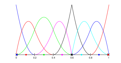
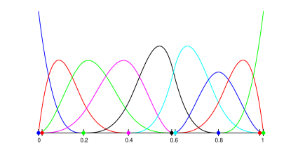
Figure 1: Example of B-splines of degree $2$ (left) and $3$ (right).

Notice that the B-spline function $N_{i,p}$ is supported in the interval $[\xi_{i},\xi_{i+p+1}]$, and in fact its definition only depends on the knots within that interval. For this reason, we define the local knot vector $\Xi_{i,p}=\{\xi_{i},\xi_{i+1},\ldots,\xi_{i+p+1}\}$, and we will sometimes denote $N_{i,p}(\zeta)\equiv N[\Xi_{i,p}](\zeta)$.

In the context of splines, three kinds of refinement are possible, as explained in [9]:

1. $k$-refinement which corresponds to successive application of the Cox-DeBoor formula (4)–(5). Regularity is raised together with the degree: therefore, the spaces (6) are not nested under $k$-refinement but, at each step (degree and regularity elevation), the dimension of the space increases by $1$. The name $k$-refinement has been introduced in [9];

2. $h$-refinement which corresponds to mesh refinement and is obtained by knot insertion. Let $\bar{\Xi}:=\{\xi_{1},\dots,\xi_{k},\bar{\xi},\xi_{k+1},\xi_{n+p+1}\}$ be the knot vector after inserting the knot $\bar{\xi}$ in $\Xi$. Then, the new B-spline functions $\{\bar{N}_{1,p}(\zeta),\ldots,\bar{N}_{n+p+2,p}(\zeta)\}$ are constructed as follows:

   $$\bar{N}_{i,p}(\zeta)=\alpha_{i}N_{i,p}(\zeta)+(1-\alpha_{i})N_{i-1,p}(\zeta)$$ (7)

   where $\alpha_{i}=1$, if $1\leq i\leq k-p$, $\alpha_{i}=\frac{\displaystyle\bar{\xi}-\xi_{i}}{\displaystyle\xi_{i+p}-\xi_{i}}$, if $k-p+1\leq i\leq k$ and, $\alpha_{i}=0$ for $k+1\leq i\leq n+p+2$. When $\bar{\xi}$ is equal to $\xi_{k}$ or $\xi_{k+1}$ or to both, the knot insertion corresponds to reduction of the inter-element regularity at $\bar{\xi}$.

3. $p$-refinement which corresponds to the degree raising with fixed interelement regularity, and generates a sequence of nested spaces.

Assuming the maximum multiplicity of the internal knots is less than or equal to $p$, i.e., the B-spline functions are at least continuous, the derivative of the B-spline $N_{i,p}$ is a spline as well. Indeed, it belongs to the spline space $S_{p-1}(\Xi^{\prime})$, where $\Xi^{\prime}=\{\xi_{2},\ldots,\xi_{n+p}\}$ is a ($p-1$)-open knot vector. Obviously, the regularity of splines in ${S}_{p-1}(\Xi^{\prime})$ is one less than the regularity in ${S}_{p}(\Xi)$.

In the following we assume that $\xi_{1}=0$ and $\xi_{n+p+1}=1$. The domain $(0,1)$ of definition of the spline functions is the one-dimensional parametric domain. On it, the knot vector $\Xi$ induces a partition of the interval $(0,1)$ that we denote by $\mathcal{M}$. Precisely, we define $\mathcal{M}$ as the set of the knot spans $(\xi_{i},\xi_{i+1})$, $i=\lceil p/2\rceil+1,...,n+\lfloor p/2\rfloor$, that can also be empty due to knot multiplicity greater than $1$. Empty intervals still play a role in the definition of B-splines and are graphically represented as points close one to the other, as proposed in [33]. Note that in this representation of $\mathcal{M}$, the number of lines is the knot multiplicity with one exception: for each boundary knot (at 0 or 1) of an open knot vector in $\mathcal{M}$ we represent only a multiplicity of $\lfloor p/2\rfloor+1$, which is $(p+1)/2$ lines if $p$ is odd, and $p/2+1$ lines if $p$ is even (see Figure 1). The reason for this construction of $\mathcal{M}$ will be motivated in the next section.

Finally, it is worth noting the relationship between the space ${S}_{p}(\Xi)$ and the space of derivatives ${S}_{p-1}(\Xi^{\prime})$, and their respective meshes $\mathcal{M}$ and $\mathcal{M}^{\prime}$. The meshes $\mathcal{M}$ and $\mathcal{M}^{\prime}$ may differ only as regards the number of points at the boundary. Indeed, according to the definition above, if $p$ is odd both meshes coincide, and if $p$ is even the number of elements of $\mathcal{M}^{\prime}$ with respect to $\mathcal{M}$ is reduced by two, one on each side.

3.1.2 Anchors and Greville sites

In this section we present the concept of anchors and of Greville sites as points in the parametric space $(0,1)$ which may be associated to each B-spline function. Greville sites, which are also known as knot averages, are classical and can be found for instance in [30], while the concept of anchors has been introduced recently in [32].

Since splines are not interpolatory, the association of functions to points (or, as we will see, other geometric entities) is somehow more arbitrary than with Lagrangian finite elements. Anchors and Greville sites are two different choices, and we present here both. Anchors are very useful when dealing with non-tensor product extensions of splines as T-meshes, while Greville sites (and related geometric entities) carry

degrees of freedom in a more natural way.

Given a B-spline function $N_{i,p}(\zeta)$, and its local knot vector $\Xi_{i,p}=\{\xi_{i},\xi_{i+1},\ldots,\xi_{i+p+1}\}$, we set: if $p$ is odd, the anchor $A$ associated with $N_{i,p}(\zeta)$ is the central knot of $\Xi_{i,p}$. If $p$ is even, the anchor $A$ associated with $N_{i,p}(\zeta)$ is chosen to be the midpoint of the central knot span of $\Xi_{i,p}$, namely: $\zeta^{A}:=\frac{\displaystyle\xi_{i+p/2}+\xi_{i+p/2+1}}{\displaystyle 2}$. The position of the anchors for degrees $p=2$ and $p=3$ are represented in Figure 1.

Note that obviously the correspondence between anchors and B-splines functions is one to one, but different anchors $A\neq\bar{A}$ may lie at the same position $\zeta^{A}=\zeta^{\bar{A}}$. A remedy to this abuse of notation, at the cost of more complex definition, is proposed in [47] where the use of both an index and a parametric domain is proposed.

The set of anchors is denoted as $\mathcal{A}_{p}=\mathcal{A}_{p}(\Xi)$. When $p$ is odd anchors are located at all knots of the partition $\mathcal{M}$ (which may be repeated), while when $p$ is even anchors are located at midpoints of all elements in $\mathcal{M}$ (including the ones of zero area). Indeed, this fact is the reason for the definition of $\mathcal{M}$ in particular as regards to the multiplicity of boundary knots.

Most often, we will use anchors to index functions and local knot vectors. Namely, for an anchor $A\in\mathcal{A}_{p}$, $\Xi^{A}_{p}$ and $B^{A}_{p}(\zeta)$ will denote the corresponding local knot vector and B-spline function, respectively. When no confusion occurs, the subindex may be removed.

Remark 3.1

The B-splines are, in general, not interpolatory at the anchor $A\in\mathcal{A}_{p}(\Xi)$, while they are interpolatory at knots having multiplicity $p$. This always happens at $\zeta=0$ and $\zeta=1$, and happens in the interior of the parametric domain where the basis is $C^{0}$ continuous, i.e., at knots with multiplicity $p$. See e.g., Figure 1(left).

Given $A\in\mathcal{A}_{p}$, and $\Xi^{A}_{p}=\{\xi_{i},..,\xi_{i+p+1}\}$ for some $i$, then the Greville site is defined as:

$$\gamma^{A}=\frac{\xi_{i+1}+\ldots+\xi_{i+p}}{p}.$$ (8)

Unlike anchor positions, Greville sites are all different one from the other, when the multiplicities $m_{j}$ verify $m_{j}\leq p$ and thus B-splines are all continuous. The Greville sites induce a partition of the unit interval, referred as Greville mesh and denoted $\mathcal{M}_{G}$. These concepts are ubiquitous in spline theory and geometry representation. Greville sites are intimately related to control points and control polygon whose properties we briefly recall in the next section.

3.1.3 B-spline curves

A B-spline curve $\Gamma$ in $\mathbb{R}^{3}$ is defined by a parametrization in the interval $(0,1)$, in the form

$${\bf F}(\zeta)=\sum_{A\in\mathcal{A}_{p}}{\bf C}^{A}B^{A}_{p}(\zeta),\qquad 0<\xi<1,$$ (9)

where ${\bf C}^{A}\in\mathbb{R}^{3}$ are called the control points. Control points are in a one-to-one correspondence with B-spline basis functions. The piecewise linear interpolation of the control points gives the control polygon $\Gamma_{C}$. See Figure 2 for an example.

The control points ${\bf C}^{A}$ have an important role not only in the definition of the spline parametrization (15), but also in the visualization and interaction with spline geometries within CAD softwares. Indeed, it is common in CAD softwares to represent, together with the parametrized curve $\Gamma$, the control points ${\bf C}^{A}$ and the associated control polygon $\Gamma_{C}$. Typically, the CAD user defines or interacts with the control points in order to input and modify the geometry. Since the B-splines are not in general interpolatory (recall Remark 3.1), then the control polygon $\Gamma_{C}$ differs from $\Gamma$, but it is “close” to it. Precisely, $\Gamma_{C}$ converges to $\Gamma$ under $h$-refinement. This convergence is proved, e.g., in [30] and discussed here below.

We introduce the usual Lagrangian basis for piecewise linear polynomials on the Greville mesh $\mathcal{M}_{G}$, denoted by $\lambda^{A}(\cdot)$:

$$\lambda^{A}(\gamma^{A^{\prime}})=\left\{\begin{aligned} 1&\text{ if }A=A^{\prime},\\ 0&\text{ if }A\neq A^{\prime}.\\ \end{aligned}\right.$$ (10)

The control polygon $\Gamma_{C}$ is then parametrized by the mapping ${\bf F}_{C}:[0,1]\rightarrow\Gamma_{C}$ defined by

$${\bf F}_{C}(\zeta)=\sum_{A\in\mathcal{A}_{p}}{\bf C}^{A}\lambda^{A}(\zeta),\qquad 0<\xi<1,$$ (11)

that is, ${\bf F}_{C}$ and ${\bf F}$ share the same control points. When ${\bf F}$ is smooth enough, the following approximation estimate holds (see, e.g., [30, Ch. XI]):

$$\underset{\zeta\in[0,1]}{\sup}\|{\bf F}(\zeta)-{\bf F}_{C}(\zeta)\|\simeq h^{2},$$ (12)

$h$ denoting the mesh-size. In other words, $\Gamma_{C}$ approximates $\Gamma$ up to an error $O(h^{2})$ under $h$-refinement. A graphical representation of this convergence can be seen in Figure 2.

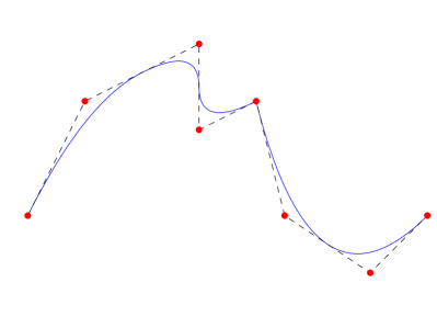
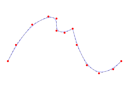
Figure 2: B-spline curve and its control polygon (left), and the same curve after one step of $h$-refinement (right).

3.2 Multivariate B-splines

Multivariate B-splines are defined from univariate B-splines by tensor product, see for instance [6, 30]. Anchors are defined in a similar way. We give here a quick overview.

3.2.1 Knot vectors, B-spline functions, anchors, Greville sites

Let $d$ be the space dimensions (in practical cases, $d=2,3$). Assume $n_{\ell}\in\mathbb{N}$, the degree $p_{\ell}\in\mathbb{N}$ and the $p_{\ell}$-open knot vector $\Xi_{\ell}=\{\xi_{\ell,1},\ldots,\xi_{\ell,n_{\ell}+p_{\ell}+1}\}$ are given, for $\ell=1,\ldots,d$. These knot vectors define a tensor product mesh $\mathcal{M}$ in the parametric domain $\widehat{\Omega}=(0,1)^{d}$ where, as in Section 3.1.2, we have to take into account the knot multiplicity. The multiplicity of a knot vector in $\Xi_{\ell}$ is represented graphically by lines ($d=2$) or planes ($d=3$) one close to the other, while the boundary is treated exactly as in one dimension.

The set of anchors is defined on $\mathcal{M}$ as the Cartesian product $\mathcal{A}_{p_{1},\ldots,p_{d}}(\Xi_{1},\ldots,\Xi_{d})=\mathcal{A}_{p_{1}}(\Xi_{1})\times\ldots\times\mathcal{A}_{p_{d}}(\Xi_{d})$. Considering, for example, the trivariate case ($d=3$) and recalling the definitions from Section 3.1.2 for the univariate case, we have that: if all $p_{\ell}$ are odd the anchors lie at the vertices of the mesh; if both $p_{1}$ and $p_{2}$ are odd and $p_{3}$ is even, then the anchors are middle-points of the vertical edges of $\mathcal{M}$; if both $p_{1}$ and $p_{2}$ are even and $p_{3}$ is odd, then the anchors are centers of the horizontal faces of $\mathcal{M}$; if all $p_{\ell}$ are even the anchors lie at the center of the elements of $\mathcal{M}$, and so on. As in the univariate case, the anchors may be located at the center of zero length edges or zero area faces or empty elements, according to knot repetition. Also, the computation of the local knot vectors for each anchor follows from the univariate case. Given an anchor $A=(A_{1},A_{2},A_{3})\in\mathcal{A}_{p_{1},p_{2},p_{3}}\equiv\mathcal{A}_{p_{1},p_{2},p_{3}}(\Xi_{1},\Xi_{2},\Xi_{3})$, we have that its coordinates are $(\zeta_{1}^{A},\zeta_{2}^{A},\zeta_{3}^{A})=(\zeta^{A_{1}},\zeta^{A_{2}},\zeta^{A_{3}})$. The three local knot vectors (one in each coordinate direction) corresponding to $A$ are defined as $\Xi_{i}^{A}:=[\Xi_{i}]_{p_{i}}^{A_{i}}$ for $i=1,2,3$ and the B-spline associated to $A$ is constructed by tensor product as:

$$B^{A}_{p_{1},p_{2},p_{3}}({\boldsymbol{\zeta}})=B^{A_{1}}_{p_{1}}(\zeta_{1})B^{A_{2}}_{p_{2}}(\zeta_{2})B^{A_{3}}_{p_{3}}(\zeta_{3}).$$ (13)

with ${\boldsymbol{\zeta}}=(\zeta_{1},\zeta_{2},\zeta_{3})\in\widehat{\Omega}=(0,1)^{3}$.

The B-spline functions (13) span the space ${S}_{p_{1},p_{2},p_{3}}(\Xi_{1},\Xi_{2},\Xi_{3})$ (or simply ${S}_{p_{1},p_{2},p_{3}}$), which is the space of piecewise polynomials of degree $p_{\ell}$ in the $x_{\ell}$ direction on $\mathcal{M}$, whose continuity at the internal mesh plane $\zeta_{\ell}=\xi_{\ell,k}$ is $C^{p_{\ell}-m_{\ell,k}}$, $m_{\ell,k}$ being the multiplicity of $\xi_{\ell,k}$ in the knot vector $\Xi_{\ell}$.

To each anchor $A\in\mathcal{A}_{p_{1},p_{2},p_{3}}(\Xi_{1},\Xi_{2},\Xi_{3})$ (or, equivalently, to each B-spline function (13)) we also associate a Greville site in the natural way, that is

$$\boldsymbol{\gamma}^{A}=(\gamma_{1}^{A},\gamma_{2}^{A},\gamma_{3}^{A})$$ (14)

where each $\gamma_{i}^{A}$ is defined as in (8), from the local knot vector $\Xi^{A}_{i}$. Connecting adjacent Greville sites, we obtain the Greville mesh $\mathcal{M}_{G}$, which is a regular tensor product mesh with all elements of positive volume.

3.2.2 Spline and NURBS geometries, multi-patch domains

Analogously to spline curves, a trivariate single-patch spline parametrization of the domain $\Omega\subset\mathbb{R}^{3}$ is ${\bf F}:\widehat{\Omega}\rightarrow\Omega$ defined as a linear combination of B-splines,

$${\bf F}({\boldsymbol{\zeta}})=\sum_{A\in\mathcal{A}_{p_{1},p_{2},p_{3}}}{\bf C}^{A}B^{A}_{p_{1},p_{2},p_{3}}({\boldsymbol{\zeta}}),\qquad\text{with }{\boldsymbol{\zeta}}\in\widehat{\Omega},$$ (15)

where ${\bf C}^{A}\in\mathbb{R}^{3}$ are called control points. In a similar way, it is also possible to define bivariate spline domains in $\mathbb{R}^{2}$ or surfaces in $\mathbb{R}^{3}$, which are commonly used in CAD (see, e.g., [6, 29]).

The control points ${\bf C}^{A}$ have again the same important role in the visualization and interaction with geometries within CAD softwares. Now, the concept of control polygon generalizes to the control mesh $\mathsf{M}_{C}$, that is, the mesh connecting the control points. Figure 3 shows an example geometry, with its control points and control mesh. The control mesh defines a polyhedral domain, denoted $\Omega_{C}$, which is an approximation of $\Omega$: again, the control domain $\Omega_{C}$ converges to $\Omega$ under $h$-refinement.

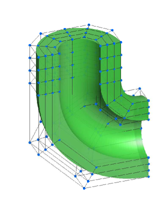
Figure 3: Representation of a geometry (green), with its control points (blue) and control mesh (black lines) for splines of degree $3$.

This is stated as in the univariate case: we introduce the usual Lagrangian basis for piecewise trilinear polynomials on the tridimensional Greville mesh $\mathcal{M}_{G}$, still denoted by $\lambda^{A}(\cdot)$, for the sake of brevity,

$$\lambda^{A}(\boldsymbol{\gamma}^{A^{\prime}})=\left\{\begin{aligned} 1&\text{ if }A=A^{\prime},\\ 0&\text{ if }A\neq A^{\prime}.\\ \end{aligned}\right.$$

The control mesh $\mathsf{M}_{C}$ is the image of the Greville mesh $\mathcal{M}_{G}$ through the piecewise trilinear mapping ${\bf F}_{C}:\widehat{\Omega}\rightarrow\Omega_{C}$,

$${\bf F}_{C}({\boldsymbol{\zeta}})=\sum_{A\in\mathcal{A}_{p_{1},p_{2},p_{3}}}{\bf C}^{A}\lambda^{A}({\boldsymbol{\zeta}}),\qquad\text{with }{\boldsymbol{\zeta}}\in\widehat{\Omega},$$ (16)

which is a parametrization of $\Omega_{C}$, since

$${\bf F}_{C}(\boldsymbol{\gamma}^{A})={\bf C}^{A}.$$

When ${\bf F}$ is smooth enough, as for (12), we have

$$\underset{{\boldsymbol{\zeta}}\in\widehat{\Omega}}{\sup}\|{\bf F}({\boldsymbol{\zeta}})-{\bf F}_{C}({\boldsymbol{\zeta}})\|\simeq h^{2}.$$ (17)

The control mesh plays a fundamental role in structural mechanics applications where the unknowns are sought as displacements of control points. In our work, we will show how this interpretation can be used also in other contexts.

Remark 3.2

When $p_{1}=p_{2}=p_{3}=1$ (and all anchors have multiplicity one) the Greville sites coincide with the anchor representations, i.e., $\boldsymbol{\gamma}^{A}={\boldsymbol{\zeta}}^{A}$, and ${\bf F}({\boldsymbol{\zeta}})={\bf F}_{C}({\boldsymbol{\zeta}})$, $\forall{\boldsymbol{\zeta}}\in\widehat{\Omega}$, that is, $\Omega_{C}$ and $\Omega$ coincide.

In CAD and isogeometric analysis the geometry is often parametrized by Non Uniform Rational B-splines (NURBS). NURBS are generated from projective transformations of splines (see [6]). A trivariate single-patch NURBS parametrization of the domain $\Omega\subset\mathbb{R}^{3}$ is a function ${\bf F}:\widehat{\Omega}\rightarrow\Omega$ defined as quotient of linear combination of B-splines,

$${\bf F}({\boldsymbol{\zeta}})=\frac{\sum_{A\in\mathcal{A}_{p_{1},p_{2},p_{3}}}{\bf C}^{A}w^{A}B^{A}_{p_{1},p_{2},p_{3}}({\boldsymbol{\zeta}})}{\sum_{A^{\prime}\in\mathcal{A}_{p_{1},p_{2},p_{3}}}w^{A^{\prime}}B^{A^{\prime}}_{p_{1},p_{2},p_{3}}({\boldsymbol{\zeta}})},\qquad{\boldsymbol{\zeta}}\in\widehat{\Omega},$$ (18)

where ${\bf C}^{A}$ are the NURBS control points and $w^{A}$ the positive NURBS weights.

In order to enhance flexibility and allow for more complex geometries, the definition of tensor-product spline and NURBS parametrized domain can be generalized to domains that are union of $N$ images of cubes; precisely

$$\text{closure }(\Omega)=\bigcup_{k=1,\ldots,N}\text{closure }(\Omega_{k})$$ (19)

where the $\Omega_{k}={\bf F}_{k}(\widehat{\Omega})$ are referred to as patches, and are assumed to be disjoint. Each patch has its own parametrization ${\bf F}_{k}$, defined on its own spline or NURBS space. The whole $\Omega$ is then referred to as a multi-patch domain. For the construction of discrete fields on a multi-patch domain $\Omega$ we will introduce in Section 4.4 suitable conformity assumptions. These will restrict the framework to configurations where it is easy to implement the proper continuity of the fields at the patches interface.

In this paper, $\Omega$ is assumed to be parametrized either by spline or NURBS functions but the unknown fields are always constructed by splines. This means that, in case of NURBS geometries, we leave the isoparametric concept which is a fundamental assumption for isogeometric methods in the context of continuum mechanics (see [8]).

4 The spline complex

This section is devoted to present the spline spaces that are compatible with the De Rham complex. The definition of the spaces is taken from [22], and is given in three dimensions (though the same construction is generalizable to arbitrary dimension). We first recall the construction on the parametric domain $\widehat{\Omega}$, and then the discrete spaces on the physical domain $\Omega$ are obtained by the push-forward mapping associated to (1). As shown in [22], it is also possible to complement these spaces with commuting and continuous projectors, in the setting of the so called Finite Element Exterior Calculus (see [2]), however this issue is not discussed here. Instead, we discuss the selection of a suitable basis for the implementation of the proposed spaces, and the meaning of the associated degrees-of-freedom. We will see that the proposed spline spaces are a natural high-order extension of classical low-order Nédélec hexahedral finite elements of the first family (see [48]), obtained in this setting for degree $p_{1}=p_{2}=p_{3}=1$, and that in a natural way they are related to cochain or chain complexes of the mesh where they are defined.

4.1 Complex on the parametric domain $\widehat{\Omega}$

We recall the following property of univariate splines, from Section 3.1.1: the derivative of a (continuous) spline is a spline, and in particular

$$\begin{CD}{S_{p}(\Xi)}@ >\frac{d}{d\zeta}>>{S_{p-1}(\Xi^{\prime})},\end{CD}$$ (20)

where $\Xi^{\prime}$ is the $(p-1)$-open knot vector that coincides with the $p$-open knot vector $\Xi$ except for the boundary knot repetitions. Moreover, we have that the derivative of the B-spline associated to an anchor $A$ in $\mathcal{A}_{p}(\Xi)$ is a linear combination of the B-splines associated to the previous and next adjacent anchors $A^{-}$ and $A^{+}$ in $\mathcal{A}_{p-1}(\Xi^{\prime})$ (only one adjacent anchor for the first and last $A\in\mathcal{A}_{p}(\Xi)$); precisely, denoting by $\Xi_{p}^{A}$ the local knot vector (formed by $p+2$ knots) of $A$ and by $\Xi_{p-1}^{A^{\pm}}$ the local knot vectors (formed by $p+1$ knots) of $A^{\pm}$, and with the general notation of Section 3.1.1, we have

$$\frac{d}{d\zeta}N[\Xi_{p}^{A}](\cdot)=\frac{p}{|\Xi_{p-1}^{A^{-}}|}N[\Xi_{p-1}^{A^{-}}](\cdot)-\frac{p}{|\Xi_{p-1}^{A^{+}}|}N[\Xi_{p-1}^{A^{+}}](\cdot),$$ (21)

where $|\Xi_{p-1}^{A^{\pm}}|$ are the length of the support of the $(p-1)$-degree B-splines $N[\Xi_{p-1}^{A^{\pm}}]$, that is, the difference of the last and first knots in the local knot vectors $\Xi_{p-1}^{A^{\pm}}$. An example is given in Figure 4. When $A$ is the first (resp., last) anchor, (21) holds with $N[\Xi_{p-1}^{A^{-}}]=0$ (resp., $N[\Xi_{p-1}^{A^{+}}]=0$). This is a well known property of B-splines (see [6, 30]) that also suggests the following scaling of the basis functions of $S_{p}(\Xi)$ and $S_{p-1}(\Xi^{\prime})$

$$S_{p}(\Xi)=\text{span}\left\{B^{A}_{p}(\cdot)\equiv N[\Xi_{p}^{A}](\cdot):\,A\in\mathcal{A}_{p}(\Xi)\right\},$$ (22)

$$S_{p-1}(\Xi^{\prime})=\text{span}\left\{D^{A}_{p-1}(\cdot)=\frac{p}{|\Xi_{p-1}^{A}|}N[\Xi_{p-1}^{A}](\cdot):\,A\in\mathcal{A}_{p-1}(\Xi^{\prime})\right\}.$$ (23)

The scaling in (23) gives the Curry-Schoenberg B-splines (see [30, Ch. IX]), that have been already used in isogeometric analysis in [28]. Indeed, with the bases (22) and (23), the matrix associated to the operator $\frac{d}{d\zeta}$ is the edge-vertex incidence matrix related to the mesh $\mathcal{M}$, when $p$ is odd, or the vertex-edge incidence matrix related to $\mathcal{M}$, when $p\geq 2$ is even. We recall that $\mathcal{M}$ also contains zero length edges and repeated vertices.

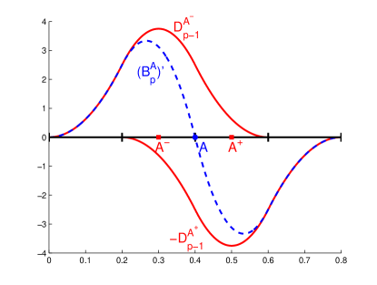
g

Figure 4: Derivative of the spline associated to the anchor $A$ as a linear combination of the splines associated to $A^{-}$ and $A^{+}$.

The observations above are the key ingredients of the trivariate construction. Following [22], and using the notation of Section 3.2, we introduce the following discrete spaces on the parametric domain $\widehat{\Omega}$

$$\widehat{X}^{0}_{h} :=S_{p_{1},p_{2},p_{3}}(\Xi_{1},\Xi_{2},\Xi_{3}),$$ (24)

$$\widehat{X}^{1}_{h} :=S_{p_{1}-1,p_{2},p_{3}}(\Xi^{\prime}_{1},\Xi_{2},\Xi_{3})\times S_{p_{1},p_{2}-1,p_{3}}(\Xi_{1},\Xi^{\prime}_{2},\Xi_{3})\times S_{p_{1},p_{2},p_{3}-1}(\Xi_{1},\Xi_{2},\Xi^{\prime}_{3}),$$

$$\widehat{X}^{2}_{h} :=S_{p_{1},p_{2}-1,p_{3}-1}(\Xi_{1},\Xi^{\prime}_{2},\Xi^{\prime}_{3})\times S_{p_{1}-1,p_{2},p_{3}-1}(\Xi^{\prime}_{1},\Xi_{2},\Xi^{\prime}_{3})\times S_{p_{1}-1,p_{2}-1,p_{3}}(\Xi^{\prime}_{1},\Xi^{\prime}_{2},\Xi_{3}),$$

$$\widehat{X}^{3}_{h} :=S_{p_{1}-1,p_{2}-1,p_{3}-1}(\Xi^{\prime}_{1},\Xi^{\prime}_{2},\Xi^{\prime}_{3}).$$

From (20), they form a De Rham complex:

$$\setcounter{MaxMatrixCols}{11}\begin{CD}\mathbb{R}@>{}>{}>\widehat{X}^{0}_{h}@>{\widehat{\,}{\bf grad}\,}>{}>\widehat{X}^{1}_{h}@>{\widehat{\,}{\bf curl}\,}>{}>\widehat{X}^{2}_{h}@>{\widehat{\,}{\rm div}\,}>{}>\widehat{X}^{3}_{h}@>{}>{}>0.\end{CD}$$ (25)

Moreover, we have the following result.

Theorem 4.1

The sequence (25) is exact.

Proof 1

This result has been already presented in [22]. We present an alternative proof, that will be useful Section 5.3.

We have to show that in (25) it holds

$$\mathbb{R}=\mathrm{ker}(\widehat{\,}{\bf grad}\,),$$ (26)

$$\mathrm{im}(\widehat{\,}{\bf grad}\,)=\mathrm{ker}(\widehat{\,}{\bf curl}\,),$$ (27)

$$\mathrm{im}(\widehat{\,}{\bf curl}\,)=\mathrm{ker}(\widehat{\,}{\rm div}\,),$$ (28)

$$\mathrm{im}(\widehat{\,}{\rm div}\,)=\widehat{X}^{3}_{h}.$$ (29)

In particular, we have to prove the inclusion $\supseteq$ in (26)–(29), since the other inclusion $\subseteq$ is trivial in all cases. It is also trivial that

$$\mathbb{R}\supseteq\mathrm{ker}(\widehat{\,}{\bf grad}\,).$$

Let $\widehat{\bf u}=(\widehat{u}_{1},\widehat{u}_{2},\widehat{u}_{3})\in\widehat{X}^{1}_{h}$, then define

$$\widehat{\phi}(\zeta_{1},\zeta_{2},\zeta_{3})=\int_{0}^{\zeta_{1}}\widehat{u}_{1}(\eta,0,0)\,d\eta+\int_{0}^{\zeta_{2}}\widehat{u}_{2}(\zeta_{1},\eta,0)\,d\eta+\int_{0}^{\zeta_{3}}\widehat{u}_{3}(\zeta_{1},\zeta_{2},\eta)\,d\eta;$$ (30)

it is easy to check that $\widehat{\bf u}=\widehat{\,}{\bf grad}\,\widehat{\phi}$ when $\widehat{\,}{\bf curl}\,{\bf u}=\boldsymbol{0}$, and that $\widehat{\phi}\in\widehat{X}^{0}_{h}$; then

$$\mathrm{im}(\widehat{\,}{\bf grad}\,)\supseteq\mathrm{ker}(\widehat{\,}{\bf curl}\,).$$

Consider $\widehat{\varphi}\in\widehat{X}^{3}_{h}$, and define $\widehat{\bf v}=(\widehat{v}_{1},0,0)\in\widehat{X}^{1}_{h}$ such that

$$\widehat{v}_{1}(\zeta_{1},\zeta_{2},\zeta_{3})=\int_{0}^{\zeta_{1}}\widehat{\varphi}(\eta,\zeta_{2},\zeta_{3})\,d\eta,$$ (31)

as before, it is easy to check that $\widehat{\varphi}=\widehat{\,}{\rm div}\,\widehat{\bf v}$ and that $\widehat{\bf v}\in\widehat{X}^{2}_{h}$; then

$$\mathrm{im}(\widehat{\,}{\rm div}\,)\supseteq\widehat{X}^{3}_{h}.$$

In order to complete the proof we need to show that

$$\mathrm{im}(\widehat{\,}{\bf curl}\,)\supseteq\mathrm{ker}(\widehat{\,}{\rm div}\,),$$

which is implied by

$$\mathrm{dim}(\mathrm{im}(\widehat{\,}{\bf curl}\,))=\mathrm{dim}(\mathrm{ker}(\widehat{\,}{\rm div}\,)).$$ (32)

To count dimensions recall from Section 3.1.1 that $\mathrm{dim}(S_{p_{\ell}}(\Xi_{\ell}))=n_{\ell}$, $\mathrm{dim}(S_{p_{\ell}-1}(\Xi^{\prime}_{\ell}))=n_{\ell}-1$; then from Section 3.2 and from (24) we get

$$\mathrm{dim}(\widehat{X}^{0}_{h}) =n_{1}n_{2}n_{3},$$ (33)

$$\mathrm{dim}(\widehat{X}^{1}_{h}) =(n_{1}-1)n_{2}n_{3}+n_{1}(n_{2}-1)n_{3}+n_{1}n_{2}(n_{3}-1),$$

$$\mathrm{dim}(\widehat{X}^{2}_{h}) =n_{1}(n_{2}-1)(n_{3}-1)+(n_{1}-1)n_{2}(n_{3}-1)+(n_{1}-1)(n_{2}-1)n_{3},$$

$$\mathrm{dim}(\widehat{X}^{3}_{h}) =(n_{1}-1)(n_{2}-1)(n_{3}-1).$$

Then, by (26)–(27),

$$\mathrm{dim}(\mathrm{im}(\widehat{\,}{\bf curl}\,)) =\mathrm{dim}(\widehat{X}^{1}_{h})-\mathrm{dim}(\mathrm{ker}(\widehat{\,}{\bf curl}\,))$$

$$=\mathrm{dim}(\widehat{X}^{1}_{h})-\mathrm{dim}(\mathrm{im}(\widehat{\,}{\bf grad}\,))$$

$$=\mathrm{dim}(\widehat{X}^{1}_{h})-\mathrm{dim}(\widehat{X}^{0}_{h})+\mathrm{dim}(\mathbb{R})$$

$$=2n_{1}n_{2}n_{3}-n_{2}n_{3}-n_{1}n_{3}-n_{1}n_{2}+1$$

and by (29)

$$\mathrm{dim}(\mathrm{ker}(\widehat{\,}{\rm div}\,)) =\mathrm{dim}(\widehat{X}^{2}_{h})-\mathrm{dim}(\mathrm{im}(\widehat{\,}{\rm div}\,))$$

$$=\mathrm{dim}(\widehat{X}^{2}_{h})-\mathrm{dim}(\widehat{X}^{3}_{h})$$

$$=2(n_{1}-1)(n_{2}-1)(n_{3}-1)+(n_{2}-1)(n_{3}-1)+(n_{1}-1)(n_{3}-1)+(n_{1}-1)(n_{2}-1)$$

$$=2n_{1}n_{2}n_{3}-n_{2}n_{3}-n_{1}n_{3}-n_{1}n_{2}+1,$$

which gives (32), and as a consequence (28).

We now show how suitable basis functions for the spaces can be constructed and as well associated to geometric entities of the mesh $\mathcal{M}$ by using the concept of anchors. We focus on basis functions first, and inspired by (22)–(23) we define them as follows:

$$\widehat{X}^{0}_{h}=\text{span}\left\{\boldsymbol{\zeta}\mapsto B^{A_{1}}_{p_{1}}(\zeta_{1})B^{A_{2}}_{p_{2}}(\zeta_{2})B^{A_{3}}_{p_{3}}(\zeta_{3}):\,A=(A_{1},A_{2},A_{3})\in\mathcal{A}_{p_{1},p_{2},p_{3}}(\Xi_{1},\Xi_{2},\Xi_{3})\right\},$$ (34)

$$\widehat{X}^{1}_{h} =\text{span }I\cup II\cup III,\text{ with}$$ (35)

$$I =\left\{\boldsymbol{\zeta}\mapsto D^{A_{1}}_{p_{1}-1}(\zeta_{1})B^{A_{2}}_{p_{2}}(\zeta_{2})B^{A_{3}}_{p_{3}}(\zeta_{3})\widehat{\bf e}_{1}:\,A=(A_{1},A_{2},A_{3})\in\mathcal{A}_{p_{1}-1,p_{2},p_{3}}(\Xi^{\prime}_{1},\Xi_{2},\Xi_{3})\right\},$$

$$II =\left\{\boldsymbol{\zeta}\mapsto B^{A_{1}}_{p_{1}}(\zeta_{1})D^{A_{2}}_{p_{2}-1}(\zeta_{2})B^{A_{3}}_{p_{3}}(\zeta_{3})\widehat{\bf e}_{2}:\,A=(A_{1},A_{2},A_{3})\in\mathcal{A}_{p_{1},p_{2}-1,p_{3}}(\Xi_{1},\Xi^{\prime}_{2},\Xi_{3})\right\},$$

$$III =\left\{\boldsymbol{\zeta}\mapsto B^{A_{1}}_{p_{1}}(\zeta_{1})B^{A_{2}}_{p_{2}}(\zeta_{2})D^{A_{3}}_{p_{3}-1}(\zeta_{3})\widehat{\bf e}_{3}:\,A=(A_{1},A_{2},A_{3})\in\mathcal{A}_{p_{1},p_{2},p_{3}-1}(\Xi_{1},\Xi_{2},\Xi^{\prime}_{3})\right\},$$

$$\widehat{X}^{2}_{h} =\text{span }I\cup II\cup III,\text{ with}$$ (36)

$$I =\left\{\boldsymbol{\zeta}\mapsto B^{A_{1}}_{p_{1}}(\zeta_{1})D^{A_{2}}_{p_{2}-1}(\zeta_{2})D^{A_{3}}_{p_{3}-1}(\zeta_{3})\widehat{\bf e}_{1}:\,A=(A_{1},A_{2},A_{3})\in\mathcal{A}_{p_{1},p_{2}-1,p_{3}-1}(\Xi_{1},\Xi^{\prime}_{2},\Xi^{\prime}_{3})\right\},$$

$$II =\left\{\boldsymbol{\zeta}\mapsto D^{A_{1}}_{p_{1}-1}(\zeta_{1})B^{A_{2}}_{p_{2}}(\zeta_{2})D^{A_{3}}_{p_{3}-1}(\zeta_{3})\widehat{\bf e}_{2}:\,A=(A_{1},A_{2},A_{3})\in\mathcal{A}_{p_{1}-1,p_{2},p_{3}-1}(\Xi^{\prime}_{1},\Xi_{2},\Xi^{\prime}_{3})\right\},$$

$$III =\left\{\boldsymbol{\zeta}\mapsto D^{A_{1}}_{p_{1}-1}(\zeta_{1})D^{A_{2}}_{p_{2}-1}(\zeta_{2})B^{A_{3}}_{p_{3}}(\zeta_{3})\widehat{\bf e}_{3}:\,A=(A_{1},A_{2},A_{3})\in\mathcal{A}_{p_{1}-1,p_{2}-1,p_{3}}(\Xi^{\prime}_{1},\Xi^{\prime}_{2},\Xi_{3})\right\},$$

$$\widehat{X}^{3}_{h}=\text{span}\left\{\boldsymbol{\zeta}\mapsto D^{A_{1}}_{p_{1}-1}(\zeta_{1})D^{A_{2}}_{p_{2}-1}(\zeta_{2})D^{A_{3}}_{p_{3}-1}(\zeta_{3}):\,A=(A_{1},A_{2},A_{3})\in\mathcal{A}_{p_{1}-1,p_{2}-1,p_{3}-1}(\Xi^{\prime}_{1},\Xi^{\prime}_{2},\Xi^{\prime}_{3})\right\},$$ (37)

where $\{\widehat{\bf e}_{\ell}\}_{\ell=1,2,3}$ denote the canonical basis of $\mathbb{R}^{3}$. We remark that all basis functions defined in (34)-(37) are non-negative.

We discuss now the association of the anchors of the bases (34)–(37) to the mesh $\mathcal{M}$ that is associated to $\widehat{X}^{0}_{h}$, that is, obtained from the knot vectors $\Xi_{1},\Xi_{2},\Xi_{3}$. We focus on the relevant case $p=p_{1}=p_{2}=p_{3}$ and consider two possible choices: $p$ is odd, or $p$ is even.

When $p$ is odd, as an immediate consequence of the definition of anchors in one space dimension, we have that:

• anchors associated with $\widehat{X}^{0}_{h}$ are $\mathcal{A}_{p,p,p}(\Xi_{1},\Xi_{2},\Xi_{3})$, which are located at the vertices of $\mathcal{M}$, i.e., there is one degree of freedom per vertex;

• anchors associated with $\widehat{X}^{1}_{h}$ are located at edges of $\mathcal{M}$ and there is one degree of freedom per edge. Indeed, e.g., anchors associated with the first component of the space $\widehat{X}^{1}_{h}$, which is $S_{p-1,p,p}(\Xi^{\prime}_{1},\Xi_{2},\Xi_{3})$, are $\mathcal{A}_{p-1,p,p}(\Xi^{\prime}_{1},\Xi_{2},\Xi_{3})$ and are located at the edges oriented as $\widehat{\bf e}_{1}$. This means that to each edge of the mesh a is associated a basis function tangential to the edge.

• anchors associated with $\widehat{X}^{2}_{h}$ are located at faces and there is one anchor per face. More in detail, if we consider the first component of $\widehat{X}^{2}_{h}$, which is $S_{p,p-1,p-1}(\Xi_{1},\Xi^{\prime}_{2},\Xi^{\prime}_{3})$, the corresponding anchors are $\mathcal{A}_{p,p-1,p-1}(\Xi_{1},\Xi^{\prime}_{2},\Xi^{\prime}_{3})$ and are located at the barycenter of the faces $f$ such that $f$ is orthogonal to $\widehat{\bf e}_{1}$. This means that a basis functions normal to the face is associated to the face.

• anchors associated with $\widehat{X}^{3}_{h}$ are $\mathcal{A}_{p-1,p-1,p-1}(\Xi^{\prime}_{1},\Xi^{\prime}_{2},\Xi^{\prime}_{3})$ and located at barycentres of all elements of $\mathcal{M}$.

We now turn to the case when of even degree $p\geq 2$, $p_{1}=p_{2}=p_{3}=p$. Note that, according to our definition, and as explained in Section 3.1.1, the meshes corresponding to the spaces $\widehat{X}^{1}_{h}$, $\widehat{X}^{2}_{h}$ and $\widehat{X}^{3}_{h}$ differ from $\mathcal{M}$ due to the different number of repeated lines at the boundary. Instead of working with different meshes for different spaces, equivalently, we represent in this case too the anchors of all spaces on the mesh $\mathcal{M}$ of $\widehat{X}^{0}_{h}$, keeping into account only the interior geometrical entities for the representations of anchors of $\widehat{X}^{1}_{h}$, $\widehat{X}^{2}_{h}$ and $\widehat{X}^{3}_{h}$.

Using the definition of anchors we immediately deduce the following:

• anchors associated with $\widehat{X}^{0}_{h}$ are at the barycentres of all elements in $\mathcal{M}$;

• anchors associated with $\widehat{X}^{1}_{h}$ are attached to the barycentres of internal faces of $\mathcal{M}$ and the corresponding vector basis function is normal to the face;

• anchors associated with $\widehat{X}^{2}_{h}$ are attached to internal edges of $\mathcal{M}$ and the corresponding vector basis function is tangent to its corresponding edge;

• anchors associated with $\widehat{X}^{3}_{h}$ are attached to internal vertices of $\mathcal{M}$.

Clearly, the positivity of the bases induces an orientation of edges and faces of the mesh $\mathcal{M}$.

With the bases (34)–(37), the discrete differential operators in (25) are represented by incidence matrices for the corresponding geometrical entities. If $p\equiv p_{1}=p_{2}=p_{3}$ is odd, then the operator $\widehat{\,}{\bf grad}\,$ is represented by the edge-vertex incidence matrix of $\mathcal{M}$ and when $p\geq 2$ is even, by the face-element incidence matrix of $\mathcal{M}$. We observe that, unlike in compatible finite elements, the matrices representing the differential operators in the selected bases (34)–(37) are essentially independent of the degree.

The fundamental consequence of the observations above is stated in the following proposition.

Proposition 4.2

The following holds:

• The spline complex (25) for odd degree $p$ is isomorphic to the cochain complex associated with the partition $\mathcal{M}$.

• The spline complex (25) for even degree $p$ is isomorphic to the chain complex associated with the partition $\mathcal{M}$ without its boundary, that is, when only the interior geometrical entities (faces, edges and vertices) are taken into account, as seen above.

As a matter of fact, this observation, together with the structure of the matrix representation of differential operators, makes the geometry of the spline complex for odd degree $p$ very similar, if not equal, to the one of the finite element complex of lowest order. However the spline complex for $p\geq 1$ delivers an approximation which is far superior than the one of low order finite element.

For $p$ even we have instead a chain complex without explicitly constructing the dual mesh, which has no analogue in the finite element framework.

Moreover, the use of anchors and the structure of the mesh at the boundary guarantee that in both the chain and cochain complex the boundary is treated in a simple and canonical way. In the case of finite elements this is not case (see e.g. [49], [50, 51], [52] or [53] ) and, moreover, these features can hardly be obtained in conjunction with high-order finite element techniques. Discretization methods based on the use of both chain and cochain complexes in the framework of isogeometric methods are very promising and object of on-going research.

We conclude this section with a remark on boundary conditions. Consider the case when homogeneous boundary conditions are imposed on the whole boundary $\partial\widehat{\Omega}$, leading to the definition of the discrete spaces $\widehat{X}^{0}_{0,h}:=\widehat{X}^{0}_{h}\cap\,{H}^{1}_{0}(\widehat{\Omega})\,$, $\widehat{X}^{1}_{0,h}:=\widehat{X}^{1}_{h}\cap\,{\bf H}_{0}(\mathbf{curl};{\widehat{\Omega}})\,$, $\widehat{X}^{2}_{0,h}:=\widehat{X}^{2}_{h}\cap\,{\bf H}_{0}({\rm div};{\widehat{\Omega}})\,$ and $\widehat{X}^{3}_{0,h}:=\widehat{X}^{3}_{h}$. These spaces are constructed as usual, by removing the functions with non-null trace at the boundary, because univariate B-spline functions are interpolatory at the boundary, as we have discussed in Remark 3.1. The associated De Rham complex

$$\setcounter{MaxMatrixCols}{11}\begin{CD}0@>{}>{}>\widehat{X}^{0}_{0,h}@>{\widehat{\,}{\bf grad}\,}>{}>\widehat{X}^{1}_{0,h}@>{\widehat{\,}{\bf curl}\,}>{}>\widehat{X}^{2}_{0,h}@>{\widehat{\,}{\rm div}\,}>{}>\widehat{X}^{3}_{0,h}@>{\int}>{}>\mathbb{R}\end{CD}$$ (38)

is exact, as easily follows by a variation of the argument of Theorem 4.1. The same holds in more general cases, for example when the boundary conditions are imposed on a part of $\partial\widehat{\Omega}$ formed by the union of some faces of the cube $\widehat{\Omega}$. Since boundary conditions do not represent a conceptual difficulty, in order to keep the presentation as clear as possible often in our presentation we will not take them into the framework.

4.2 Push-forward to the single-patch physical domain $\Omega$

Following Section 3.2.2, we suppose that the domain $\Omega$ is obtained from $\widehat{\Omega}$ through a spline or NURBS single-patch mapping ${\bf F}$. Clearly, we need to choose the space for ${\bf F}$.

Assumption 4.3 (Isogeometric mapping)

We assume that ${\bf F}$ is either a spline function in $[\widehat{X}^{0}_{h}]^{3}$, or ${\bf F}$ is a NURBS function as in (18), with numerator in $[\widehat{X}^{0}_{h}]^{3}$ and weight denominator in $\widehat{X}^{0}_{h}$.

Assumption 4.3 is indeed very natural in the context of isogeometric methods: it means that the discrete fields are constructed from the geometry knot vectors and bases, possibly after refinement.

We denote by $\mathsf{M}$ the image of $\mathcal{M}$ through the mapping ${\bf F}$. $\mathsf{M}$ is then a partition of the physical domain $\Omega$, similar to the finite element mesh, even though it contains elements of zero area due to knot multiplicity.

The discrete spaces $X^{0}_{h},\ldots,X^{3}_{h}$ on the physical domain $\Omega$ can be defined from the spaces (24) on the parametric domain $\widehat{\Omega}$ by push-forward, that is, the inverse of the transformations defined in (1), that commute with the differential operators (as given by the diagrams (2) and (3)):

$$\setcounter{MaxMatrixCols}{11}\begin{CD}\mathbb{R}@>{}>{}>\widehat{X}^{0}_{h}@>{\widehat{\,}{\bf grad}\,}>{}>\widehat{X}^{1}_{h}@>{\widehat{\,}{\bf curl}\,}>{}>\widehat{X}^{2}_{h}@>{\widehat{\,}{\rm div}\,}>{}>\widehat{X}^{3}_{h}@>{}>{}>0\\ @A{\iota^{0}}A{}A@A{\iota^{1}}A{}A@A{\iota^{2}}A{}A@A{\iota^{3}}A{}A\\ \mathbb{R}@>{}>{}>X^{0}_{h}@>{\,{\bf grad}\,}>{}>X^{1}_{h}@>{\,{\bf curl}\,}>{}>X^{2}_{h}@>{\,{\rm div}\,}>{}>X^{3}_{h}@>{}>{}>0,\\ \end{CD}$$ (39)

that is, the discrete spaces in the physical domain are defined as

$$X^{0}_{h}:=\{\phi:\iota^{0}(\phi)\in\widehat{X}^{0}_{h}\},$$ (40)

$$X^{1}_{h}:=\{{\bf u}:\iota^{1}({\bf u})\in\widehat{X}^{1}_{h}\},$$

$$X^{2}_{h}:=\{{\bf v}:\iota^{2}({\bf v})\in\widehat{X}^{2}_{h}\},$$

$$X^{3}_{h}:=\{\varphi:\iota^{3}(\varphi)\in\widehat{X}^{3}_{h}\}.$$

We remark that the space $X^{1}_{h}$, which is a discretization of $\,{\bf H}({\mathbf{curl}};\Omega)\,$, is defined through the curl conserving transformation $\iota^{1}$, and that the space $X^{2}_{h}$, which is a discretization of $\,{\bf H}({\rm div};\Omega)\,$, is defined through the divergence conforming transformation $\iota^{2}$. These are equivalent to the curl and divergence preserving transformations that are used to define edge and face elements, respectively (see [46, Sect. 3.9]).

Thanks to the properties of the operators (1) the push-forwarded spaces $X^{0}_{h},\ldots,X^{3}_{h}$ inherit the same fundamental properties of $\widehat{X}^{0}_{h},\ldots,\widehat{X}^{3}_{h}$, that we have discussed in the previous section:

• they form an exact De Rham complex without boundary conditions

  $$\setcounter{MaxMatrixCols}{11}\begin{CD}\mathbb{R}@>{}>{}>X^{0}_{h}@>{\,{\bf grad}\,}>{}>X^{1}_{h}@>{\,{\bf curl}\,}>{}>X^{2}_{h}@>{\,{\rm div}\,}>{}>X^{3}_{h}@>{}>{}>0,\end{CD}$$ (41)

  or with boundary conditions

  $$\setcounter{MaxMatrixCols}{11}\begin{CD}0@>{}>{}>X^{0}_{0,h}@>{\,{\bf grad}\,}>{}>X^{1}_{0,h}@>{\,{\bf curl}\,}>{}>X^{2}_{0,h}@>{\,{\rm div}\,}>{}>X^{3}_{0,h}@>{\int}>{}>\mathbb{R}.\end{CD}$$ (42)

• the basis functions for $X^{0}_{h},\ldots,X^{3}_{h}$ are defined by push-forward of the basis functions of $\widehat{X}^{0}_{h},\ldots,\widehat{X}^{3}_{h}$, similarly to (40), and are in one-to one relation with the images of the anchors through ${\bf F}$. See Figure 5.

  

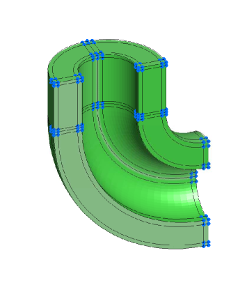
  Figure 5: We show the mesh $\mathsf{M}$ and the image of the anchors related to the space $X^{0}_{h}$ on an example geometry.

• since (39), the matrices associated with the differential operators $\,{\bf grad}\,$, $\,{\bf curl}\,$ and $\,{\rm div}\,$ on $\Omega$ are the same as the matrices of $\widehat{\,}{\bf grad}\,$, $\widehat{\,}{\bf curl}\,$ and $\widehat{\,}{\rm div}\,$ on $\widehat{\Omega}$, that is, incidence matrices of the mesh $\mathsf{M}$.

• when $p$ is odd (even, respectively), the complex ($X^{0}_{h},\ldots,X^{3}_{h}$) is isomorphic to the cochain (chain, respectively) complex associated to the partition $\mathsf{M}$.

Finally, the discrete spaces $X^{0}_{h},\ldots,X^{3}_{h}$ inherit from their pull-back $\widehat{X}^{0}_{h},\ldots,\widehat{X}^{3}_{h}$ optimal approximation properties, if the geometrical mapping ${\bf F}$ satisfies Assumption 4.3 and its inverse is smooth enough (see [22] for details).

4.3 Control fields and degrees-of-freedom interpretation

In this section, we introduce the concept of control fields, thanks to which we give an interpretation of the degrees-of-freedom of the isogeometric fields defined in Section 4.1–4.2. The control fields are for the B-spline isogeometric fields what the control mesh is for the the B-spline geometry. We recall that from the geometry control points we define ${\bf F}_{C}$ (see (16)), the piecewise trilinear function on the Greville mesh $\mathcal{M}_{G}$. The image of ${\bf F}_{C}$ is the so-called control domain $\Omega_{C}$. The so-called control mesh $\mathsf{M}_{C}$ (which is a partition of $\Omega_{C}$) is the image through ${\bf F}_{C}$ of the Greville mesh $\mathcal{M}_{G}$.

As described in Section 3.2.2, the standard way to manipulate a spline parametrization ${\bf F}$ is by moving its control points, that is, the vertices of the control mesh $\mathsf{M}_{C}$. The parametrization ${\bf F}_{C}$ or, equivalently, the control mesh $\mathsf{M}_{C}$, carries the degrees-of-freedom for the geometry. The distance between the two parametrizations ${\bf F}$ and ${\bf F}_{C}$ is at most $O(h^{2})$, as in (17). We now apply the same rationale for the complex $(X^{0}_{h},...,X^{3}_{h}\color[rgb]{0,0,0})$. Let us first focus on scalar functions on the parametric domain $\widehat{\Omega}$, i.e., on the space $\widehat{X}^{0}_{h}$. Given a spline

$$\widehat{\phi}({\boldsymbol{\zeta}})=\sum_{A\in\mathcal{A}_{p,p,p}}c^{A}B^{A}_{p,p,p}({\boldsymbol{\zeta}}),\qquad\text{with }{\boldsymbol{\zeta}}\in\widehat{\Omega},$$ (43)

where $c^{A}$ are its control variables, we associate the piecewise trilinear function defined on the mesh $\mathcal{M}_{G}$:

$$\widehat{\phi}_{C}({\boldsymbol{\zeta}})=\sum_{A\in\mathcal{A}_{p,p,p}}c^{A}\lambda^{A}({\boldsymbol{\zeta}}),\qquad\text{with }{\boldsymbol{\zeta}}\in\widehat{\Omega},$$ (44)

which carries the same degrees-of-freedom for $\widehat{\phi}$ and indeed is close to $\widehat{\phi}$ (the distance between the two functions is at most $O(h^{2})$, analogously to (12)). By this relation, we can interpret the degrees-of-freedom $c^{A}$ of $\widehat{\phi}$ as the values of $\widehat{\phi}_{C}$ at each Greville site in $\mathcal{M}_{G}$.

It should be noted that, if the values of these degrees-of-freedom are chosen wisely, splines deliver approximation error of order $O(h^{p})$ in the norm of $H^{1}(\widehat{\Omega})$, where $p$ is the degree of the spline, while the corresponding trilinear function can only provide approximation errors of order $O(h)$.

Let now the geometry come into play. Using (40), we set:

$$\phi\circ{\bf F}=\widehat{\phi}\text{ and }\phi_{C}\circ{\bf F}_{C}=\widehat{\phi}_{C}.$$ (45)

The degrees-of-freedom for $\phi$ are the values of $\phi_{C}$ at the vertices of $\mathsf{M}_{C}$, that is, at the control points. Or, we can say that the field $\phi_{C}$ determines, or controls, $\phi$, and its degrees-of-freedom are the values of $\phi_{C}$ at control points. In Figure 3, the location of control points (blue bullet) is shown on an example geometry. The field $\phi_{C}$ plays the role of control field for $\phi$. As for the parametric space, there are wise choices of the degrees-of-freedom which ensure an approximation error of order $O(h^{p})$ in the norm of $H^{1}(\Omega)$, while the corresponding trilinear function can only provide approximation errors of order $O(h)$.

The same reasoning can be applied to the whole complex $(X^{0}_{h},...,X^{3}_{h}\color[rgb]{0,0,0})$, defined in Section 4.1 and 4.2, from degrees $p_{\ell}$ and knot vectors $\Xi_{\ell}$. Indeed, we introduce the control complex $(Z^{0}_{h},...,Z^{3}_{h}\color[rgb]{0,0,0})$ which is obtained, still following Section 4.1 and 4.2, with the following choices for $\widehat{Z}^{0}_{h}$:

• degrees in all directions equal to $1$;

• the knot vector in the $\ell$ direction is the ordered collection of points $\{\gamma_{\ell}^{A}\ :\ A\in\mathcal{A}_{p_{\ell}}(\Xi_{\ell})\}$, $\ell=1,2,3$, along with repeated 0 and 1 to make the knot vectors open,

and replacing the geometric mapping ${\bf F}$ with ${\bf F}_{C}$ in the pullbacks (1). The complex $(Z^{0}_{h},...,Z^{3}_{h}\color[rgb]{0,0,0})$ corresponds to the low order finite element complex defined on the control mesh $\mathsf{M}_{C}$ and it is immediate to see that if $\phi$ in (45) belongs to $X^{0}_{h}$, then the corresponding $\phi_{C}$ belongs to $Z^{0}_{h}$. We denote by $I^{0}_{h}:X^{0}_{h}\to Z^{0}_{h}$ the operator which associates $\phi$ to $\phi_{C}$, and in an analogous way, we define the operators $I^{j}_{h}:X^{j}_{h}\to Z^{j}_{h}$, $j=0,\ldots,3$. These operators are represented by identity matrices when the spaces are endowed with the bases described in Section 4.1. It is not difficult to see that, in view of the structure of the matrices associated to differential operators, the following diagram commutes:

$$\setcounter{MaxMatrixCols}{11}\begin{CD}\mathbb{R}@>{}>{}>X^{0}_{h}@>{\,{\bf grad}\,}>{}>X^{1}_{h}@>{\,{\bf curl}\,}>{}>X^{2}_{h}@>{\,{\rm div}\,}>{}>X^{3}_{h}@>{}>{}>0\\ @V{I^{0}_{h}}V{}V@V{I^{1}_{h}}V{}V@V{I^{2}_{h}}V{}V@V{I^{3}_{h}}V{}V\\ \mathbb{R}@>{}>{}>Z^{0}_{h}@>{\,{\bf grad}\,}>{}>Z^{1}_{h}@>{\,{\bf curl}\,}>{}>Z^{2}_{h}@>{\,{\rm div}\,}>{}>Z^{3}_{h}@>{}>{}>0.\\ \end{CD}$$ (46)

Let us comment about the meaning of the diagram (46). First of all, it says that the geometric structure of the spline complex $(X^{0}_{h},...,X^{3}_{h}\color[rgb]{0,0,0})$ is the one of the low order finite element complex $(Z^{0}_{h},...,Z^{3}_{h}\color[rgb]{0,0,0})$ on the control mesh. The discrete fields in $X^{j}_{h}$ can be associated to control fields in $Z^{j}_{h}$, through the operator $I^{j}_{h}$, as we have discussed for $j=0$ above. For example, we can say that there is a Nédélec field ${\bf u}_{C}$ which controls ${\bf u}$ and the degrees-of-freedom are, in this case, its circulation on the edges of the control mesh $\mathsf{M}_{C}$. Moreover, following a reasoning similar to the one in Section 3.2.2, the operators $I^{j}_{h}$ are point-wise converging to the identity when $h$ goes to zero. We stress again that the order of approximation of the complex $(X^{0}_{h},...,X^{3}_{h}\color[rgb]{0,0,0})$ is $O(h^{p})$ while the control complex $(Z^{0}_{h},...,Z^{3}_{h}\color[rgb]{0,0,0})$ only exhibits first order convergence in the norm of $X^{i}$.

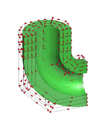
Figure 6: Representation of the degrees-of-freedom location for the space $X^{1}_{h}$, on the green geometry for degrees $p_{1}=p_{2}=p_{3}=3$.

Finally, it should be noted that, as it is well known, the complex $(Z^{0}_{h},..,Z^{3}_{h})$ is always isomorphic to the cochain complex of the partition $\mathsf{M}_{C}$, while for the complex $(X^{0}_{h},..,X^{3}_{h})$ Proposition 4.2 holds. This is in accordance with the fact that, when $p_{\ell}$ are all even, the control mesh $\mathsf{M}_{C}$ can be interpreted as a partition dual to $\mathsf{M}$, in the sense that the chain of $\mathsf{M}$ is isomorphic to the cochain complex of $\mathsf{M}_{C}$.

4.4 Push-forward to the multi-patch physical domain $\Omega$

In this section we construct the spline complex on a multi-patch geometry by addressing the questions of how conformity is imposed at the interfaces between patches.

We consider now a multi-patch domain $\Omega$ which is parametrized from a reference patch $\widehat{\Omega}$ through the spline or NURBS mappings ${\bf F}_{k}$, $k=1,\ldots,N$, as in (19). Each patch is endowed with a (possibly different) spline space and therefore for each $k=1,\ldots,N$ we can define discrete spaces $[\widehat{X}^{0}_{h}]_{k},\ldots,[\widehat{X}^{3}_{h}]_{k}$ such that a De Rham complex (25) holds. Assuming each ${\bf F}_{k}$ verifies Assumption 4.3, then, as shown in Section 4.2 we push-forward patch-by-patch the discrete spaces $[\widehat{X}^{0}_{h}]_{k},\ldots,[\widehat{X}^{3}_{h}]_{k}$ and obtain, on each $\Omega_{k}={\bf F}_{k}(\widehat{\Omega})$, the discrete spaces $[X^{0}_{h}]_{k},\ldots,[X^{3}_{h}]_{k}$ that fulfill the De Rham complex (4.2) on each patch.

Then, the last and main step is to assemble the spaces $X_{h}^{j}\subset\bigoplus_{k=1,\ldots,N}[X_{h}^{j}]_{k}$, and add the relevant continuity conditions at the inter-patches boundaries: trace continuity for $X^{0}_{h}$, tangential trace continuity for $X^{1}_{h}$, normal trace continuity for $X^{2}_{h}$, no continuity for $X^{3}_{h}$. For this purpose, we introduce a conformity condition as, e.g., in [26]. This condition guarantees that the geometry parametrizations of the patches are equivalent at the patch interfaces and, since Assumption 4.3, it can be stated on the spaces $[\widehat{X}^{0}_{h}]_{k}$.

Assumption 4.4 (Geometrical conformity)

On each non-empty patch interface $\Gamma=\partial\Omega_{k}\cap\partial\Omega_{k^{\prime}}$, with $k\neq k^{\prime}$, the spaces $[X^{0}_{h}]_{k}|_{\Gamma}$ and $[X^{0}_{h}]_{k^{\prime}}|_{\Gamma}$ coincide, as the corresponding bases do.

This means that the meshes $\mathsf{M}_{k}$ and $\mathsf{M}_{k^{\prime}}$ match on $\Gamma$, and therefore

$$\mathsf{M}=\bigcup_{k=1,\ldots,N}\mathsf{M}_{k}$$

is a locally structured but globally unstructured mesh $\mathsf{M}$ on $\Omega$. In a similar way, the patch control meshes $[\mathsf{M}_{C}]_{k}$ match conformally and

$$\mathsf{M}_{C}=\bigcup_{k=1,\ldots,N}[\mathsf{M}_{C}]_{k}$$

is a locally structured but globally unstructured mesh $\mathsf{M}_{C}$ of hexahedra on $\Omega_{C}$, the union of the patch control domains $[\Omega_{C}]_{k}$.

Assumption 4.4 corresponds to the full-matching conditions of [26], to which we refer for further details.

Having conformity we can implement the continuity conditions easily. Indeed, due to the definitions in Sections 4.1–4.3, the needed continuity holds for $(X^{0}_{h},...,X^{3}_{h})$ if and only if it holds for $(Z^{0}_{h},...,Z^{3}_{h})$ on the global mesh $\mathsf{M}_{C}$. Continuity for $Z^{0}_{h},Z^{1}_{h}$ and $Z^{2}_{h}$ is imposed by merging the coincident degrees-of-freedom at the interfaces, which in the case of $Z^{1}_{h}$ and $Z^{2}_{h}$ also requires to take into account the orientation; see Figure 7. This is however the same as in finite elements (indeed, the control fields are classical finite elements). This merging automatically gives the degrees-of-freedom for fields in $(X^{0}_{h},...,X^{3}_{h})$.

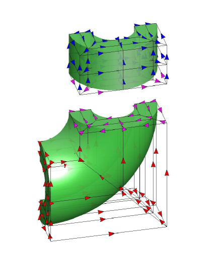
(a) Control variables of the two patches before merging.

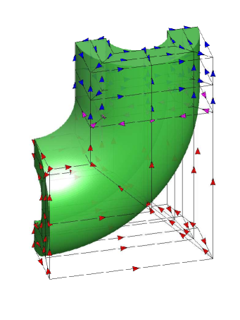
(b) Control variables of the merged patch.

Figure 7: Implementing continuity for $X^{1}_{h}$ on a two-patch domain. The orientation of the edges at the interface is chosen as that of the lower patch.

5 Beyond the tensor product structure: T-splines

In this section, we generalize the definition of tensor-product B-splines to T-splines [7, 31, 32]. The theory of T-splines is well developed in two dimensions (see the very recent papers [37, 38, 47, 54]) while it is still incomplete in three dimensions (though some recent important advances have been recently proposed in [19]). For this reason, we only present in Sections 5.1 and 5.2, T-splines in two dimensions and construct, in Section 5.3, a discrete T-spline based complex. The extension to three dimensions is given in Section 5.4 by tensor-product of the two-dimensional T-spline spaces with B-spline one-dimensional spaces.

5.1 T-mesh

Let $n_{\ell}\in\mathbb{N}$ and the degree $p_{\ell}\in\mathbb{N}$, and let $\Xi_{\ell}=\{\xi_{\ell,1},\ldots,\xi_{\ell,n_{\ell}+p_{\ell}+1}\}$ be a $p_{\ell}$-open knot vector for $\ell=1,2$. A T-mesh is a rectangular tiling of the unit square $[0,1]^{2}$, such that all vertices belong to $\Xi_{1}\times\Xi_{2}$. A T-mesh may contain interior vertices that connect only three edges, called T-junctions, that break the tensor product structure of the mesh (see Figure 10). We will say that a T-junction is horizontal (respectively, vertical) if the missing edge is horizontal (resp. vertical). By an abuse of notation, we still denote a T-mesh by $\mathcal{M}$.

As before, we represent the knot multiplicities by repeated lines close to each other, with now the line multiplicity possibly varying along lines (see [32, Section 4.3]). The only exception are the boundary lines, that maintain the same multiplicity all along the line. As in B-spline meshes, the vertical (resp. horizontal) lines at the boundaries have multiplicity $\lfloor p_{1}/2\rfloor+1$ (resp. $\lfloor p_{2}/2\rfloor+1$).

5.2 Analysis suitable T-meshes and T-splines.

We define, for a horizontal (resp. vertical) T-junction $T$, the $k$-bay face-extension as the horizontal (resp. vertical) closed segment that extends from $T$ in the direction of the missing edge until it intersects $k$ lines of the mesh $\mathcal{M}$. The $k$-bay edge-extension is defined analogously extending the segment in the opposite direction.

Following [47], we define the extension of a horizontal (resp. vertical) T-junction $T$ the union of the $\lfloor(p_{1}+1)/2\rfloor$-bay face-extension, and the $\lfloor(p_{1}-1)/2\rfloor$-bay edge-extension (resp. the union of the $\lfloor(p_{2}+1)/2\rfloor$-bay face-extension, and the $\lfloor(p_{2}-1)/2\rfloor$-bay edge-extension). More precisely, if $p_{\ell}$ is odd we extend $(p_{\ell}+1)/2$ bays in the direction of the missing edge, and $(p_{\ell}-1)/2$ bays in the opposite direction; if $p_{\ell}$ is even we extend $p_{\ell}/2$ bays in both directions. An example is given in Figure 8.

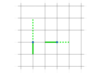
Figure 8: Extensions for degree $p_{1}=2$ (horizontal) and $p_{2}=3$ (vertical). Dashed lines represent the face extensions.

Definition 5.1

A T-mesh $\mathcal{M}$ is analysis suitable for degrees $p_{1}$ and $p_{2}$, denoted $\mathcal{M}\in\mathsf{AS}_{p_{1},p_{2}}$, if vertical extensions and horizontal extensions do not intersect.

Analysis suitable T-meshes were first identified in [37] in the bi-cubic case, and generalized to arbitrary degree in [47]. Despite their very geometric definition, analysis suitable T-meshes and T-splines enjoy fundamental properties which make their use in isogeometric analysis really promising. Some of these properties will be discussed in what follows.

As in the case of B-splines, anchors are inferred from the T-mesh $\mathcal{M}$ and their position depends upon the parity of $p_{1}$ and $p_{2}$. For example, if both $p_{1}$ and $p_{2}$ are odd, anchors are at the vertices of the $\mathcal{M}$, if they are even, anchors are at the barycenters of elements and so on (see [47]). We will denote the set of anchors by $\mathcal{A}_{p_{1},p_{2}}(\mathcal{M})$, or simply $\mathcal{A}_{p_{1},p_{2}}$.

T-spline basis functions are constructed as B-splines associated to the anchors $\mathcal{A}_{p_{1},p_{2}}(\mathcal{M})$, and defined from two local knot vectors, $\Xi_{1}^{A}=\{\xi_{1,i_{1}},\ldots,\xi_{1,i_{p_{1}+2}}\}\subset\Xi_{1}$ and $\Xi_{2}^{A}=\{\xi_{2,i_{1}},\ldots,\xi_{2,i_{p_{2}+2}}\}\subset\Xi_{2}$. To construct the horizontal knot vector $\Xi_{1}^{A}$ we trace the horizontal line through $A$ and select its intersections with vertical lines of $\mathcal{M}$, depending on the degree $p_{1}$: if $p_{1}$ is even we choose the first $(p_{1}+2)/2$ intersections to the left of $A$, and the first $(p_{1}+2)/2$ to the right; if $p_{1}$ is odd we first select the coordinate of the anchor $A$, and then the first $(p_{1}+1)/2$ intersections to the left and to the right of $A$. In the case that we arrive at the boundary, we add the value 0 or 1 as many times as needed to complete the $p_{1}+2$ entries of $\Xi_{1}^{A}$. The construction of $\Xi_{2}^{A}$ is analogous, and depends on $p_{2}$. Examples are shown in Figure 9 for $p_{1}=2$ and $p_{2}=3$. For more details we refer to [32].

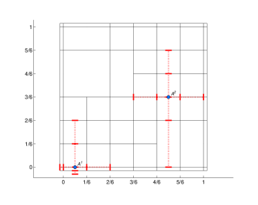
Figure 9: Representation of the local knot vectors for degrees $p_{1}=2$ and $p_{2}=3$. The local knot vectors are $\Xi_{1}^{A^{1}}=\{0,0,1/6,2/6\}$, $\Xi_{2}^{A^{1}}=\{0,0,0,1/6,2/6\}$, and $\Xi_{1}^{A^{2}}=\{3/6,4/6,5/6,1\}$, $\Xi_{2}^{A^{2}}=\{0,2/6,3/6,4/6,5/6\}$.

The T-spline function associated to the anchor $A$ is denoted as:

$$B^{A}_{p_{1},p_{2}}({\boldsymbol{\zeta}})=N[\Xi_{1}^{A}](\zeta_{1})N[\Xi_{2}^{A}](\zeta_{2}),\quad{\boldsymbol{\zeta}}=(\zeta_{1},\zeta_{2})\in(0,1)^{2},$$ (47)

they are linearly independent (see [47]) and by definition span the T-spline space $T_{p_{1},p_{2}}=T_{p_{1},p_{2}}(\mathcal{M})$:

$$T_{p_{1},p_{2}}(\mathcal{M}):=\mbox{span}\{B_{p_{1},p_{2}}^{A}\ :\ A\in\mathcal{A}_{p_{1},p_{2}}(\mathcal{M})\}.$$ (48)

Definition 5.1 guarantees fundamental properties of the T-spline space (48). In [38, 47] it is defined a dual basis for the T-spline functions constructed from an analysis suitable T-mesh, thus proving the linear independence of (47) (see also [37]) and good approximation properties for the space (48). We also remark that the construction of the local knot vectors described above is analogous to the one in [47] for analysis suitable T-meshes.

Finally, we define the extended T-mesh of $\mathcal{M}$, and denote it by $\mathcal{M}_{\rm ext}$, as the T-mesh obtained from $\mathcal{M}$ by adding all the T-junction extensions. The extended T-mesh, sometimes also called Bézier mesh, is the minimal mesh such that the functions (47) restricted to the non-empty elements are bivariate polynomials of degree $(p_{1},p_{2})$. The importance of the extended mesh for implementation [55], local refinement [54] and approximation properties of T-splines [47] is already known. In particular, for the implementation, and in order to ensure accuracy, integration has to be performed on the elements of $\mathcal{M}_{\rm ext}$ and this means that the data structure is constructed based on $\mathcal{M}_{\rm ext}$.

Finally, a key result which is useful in the construction of compatible T-spline discretizations, is the characterization stated in the following proposition.

Proposition 5.2

Given an analysis suitable T-mesh $\mathcal{M}$, if furthermore no T-junction extensions of any kind intersect each other or intersect mesh lines with multiplicity greater than one, then the T-spline space (48) is the space of all piece-wise bivariate polynomials of degree $(p_{1},p_{2})$ on $\mathcal{M}_{\rm ext}$ with the same continuity of the T-spline functions (47) at the mesh lines.

Proof 2

The case $p_{1}=p_{2}=3$ has been covered in [54], while the general case is a work in progress by A. Bressan in [56]. Related works are also [57], and [58] which show the mathematical complexity of the problem. The condition that the extensions do not intersect lines with multiplicity greater than one can be removed at the price of a more complex statement, which we do not consider here for the sake of simplicity.

5.3 Two-dimensional De Rham complex with T-splines on the parametric domain $(0,1)^{2}$

The aim of this section is to introduce a two-dimensional T-spline based De Rham complex, thus generalizing the tensor-product construction of section 4. Throughout this Section we will assume, for the sake of simplicity, $p_{1}=p_{2}=p$. The results are also valid in the general case, but the proofs become more intricate.

As for B-splines, T-splines spaces are constructed by a suitable selection of the polinomial degree in the two directions and by a suitable design of the mesh, that is, the knot vectors. The main difference now is that we need to modify the mesh $\mathcal{M}$, depending of the form degree, not only at the boundary but also around T-junctions.

Let $p\in\mathbb{N}$, let $\Xi_{1},\Xi_{2}$ be two $p$-open knot vectors, and let $\mathcal{M}\in\mathsf{AS}_{p,p}$ be a T-mesh with knot repetitions, as defined in Section 5.1. The starting mesh is ${\mathcal{M}}^{0}\equiv\mathcal{M}$, on which we define the space of scalar fields:

$$\widehat{Y}^{0}_{h}:=T_{p,p}({\mathcal{M}}^{0}).$$ (49)

The T-splines vector fields are defined on the two T-meshes ${\mathcal{M}}^{1}_{1}$ and ${\mathcal{M}}^{1}_{2}$. If $p$ is odd, ${\mathcal{M}}^{1}_{1}$ is obtained from $\mathcal{M}$ by adding the first-bay face-extension of all horizontal T-junctions. If $p$ is even, ${\mathcal{M}}^{1}_{1}$ is equal to $\mathcal{M}$ everywhere but on the boundary where, due to the definition of $\mathcal{M}$, and recalling Section 3.1.1, the first and the last vertical columns of elements of $\mathcal{M}$ are removed. We define analogously ${\mathcal{M}}^{1}_{2}$, reasoning in the vertical direction: if $p$ is odd ${\mathcal{M}}^{1}_{2}$ is defined by adding the first-bay face-extension of all the vertical T-junctions, and if $p$ is even, it is defined by removing the first and last horizontal rows of elements of $\mathcal{M}$. Then the vector fields and the rotated vector fields are defined as

$$\widehat{Y}^{1}_{h}:=T_{p-1,p}({\mathcal{M}}^{1}_{1})\times T_{p,p-1}({\mathcal{M}}^{1}_{2}).$$ (50)

$$\widehat{Y}^{1*}_{h}:=T_{p,p-1}({\mathcal{M}}^{1}_{2})\times T_{p-1,p}({\mathcal{M}}^{1}_{1}).$$ (51)

Finally, the last space $\widehat{Y}^{2}_{h}$ is defined on the T-meshes ${\mathcal{M}}^{2}$: if $p$ is odd, ${\mathcal{M}}^{2}$ is obtained from $\mathcal{M}$ by adding all the first-bay face-extensions (horizontal and vertical), and if $p$ is even it is defined by removing the first and last rows and columns of elements in $\mathcal{M}$.

Then

$$\widehat{Y}^{2}_{h}:=T_{p-1,p-1}({\mathcal{M}}^{2}).$$ (52)

An example of the sequence of meshes is shown in Figure 10 for $p=3$, and in Figure 11 for $p=2$. We notice that whenever ${\mathcal{M}}^{0}=\mathcal{M}$ is a tensor product mesh, the construction is equivalent to the one presented in Section 4.1 for B-splines. Indeed, for odd $p$ the four meshes are equal to $\mathcal{M}$, because there are no T-junctions, and for even $p$ they only differ in the number of line repetitions on the boundary.

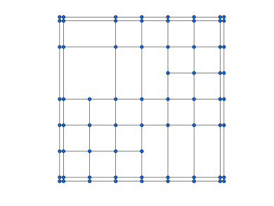
(a) Mesh ${\mathcal{M}}^{0}$

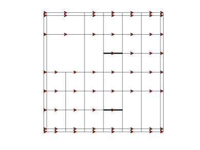
(b) Mesh ${\mathcal{M}}^{1}_{1}$

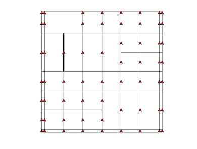
(c) Mesh ${\mathcal{M}}^{1}_{2}$

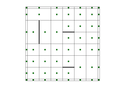
(d) Mesh ${\mathcal{M}}^{2}$

Figure 10: Sequence of meshes for the spline complex, with their respective anchors, for $p=3$.

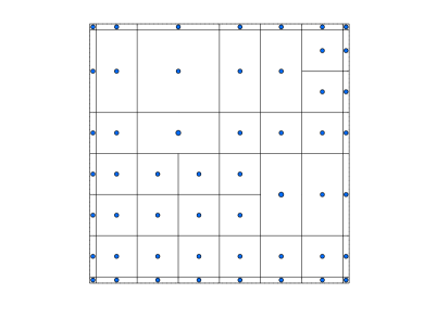
(a) Mesh ${\mathcal{M}}^{0}$

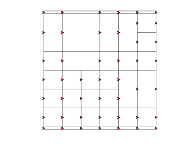
(b) Mesh ${\mathcal{M}}^{1}_{1}$

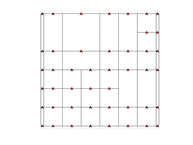
(c) Mesh ${\mathcal{M}}^{1}_{2}$

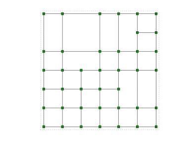
(d) Mesh ${\mathcal{M}}^{2}$

Figure 11: Sequence of meshes for the spline complex, with their respective anchors, for $p=2$.

The choice of these meshes becomes clear when computing the derivatives. For instance, let $p=3$ and consider the simple example of a mesh with only one horizontal T-junction, as in Figure 12(a). Choosing the anchor $A\in\mathcal{A}_{p,p}({\mathcal{M}}^{0})$ located at the T-junction, it is clear from (21) that $\frac{\partial B^{A}_{p,p}}{\partial x}$ is a linear combination of $B^{A^{l}}_{p-1,p}$ and $B^{A^{r}}_{p-1,p}$, with $A^{l},A^{r}\in\mathcal{A}_{p-1,p}({\mathcal{M}}^{1}_{1})$ as in Figure 12(b). Hence, $\frac{\partial B^{A}_{p,p}}{\partial x}\in T_{p-1,p}({\mathcal{M}}^{1}_{1})$ (see (50)), but since $A^{l}\not\in\mathcal{A}_{p-1,p}({\mathcal{M}}^{0})$, we have $\frac{\partial B^{A}_{p,p}}{\partial x}\not\in T_{p-1,p}({\mathcal{M}}^{0})$. The argument is analogous for the partial derivative with respect to the $y$ direction, with vertical T-junctions.

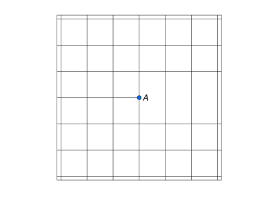
(a) Anchor $A\in\mathcal{A}_{p,p}({\mathcal{M}}^{0})$

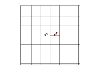
(b) Anchors $A^{l},A^{r}\in\mathcal{A}_{p-1,p}({\mathcal{M}}^{1}_{1})$

Figure 12: The first partial derivative $\frac{\partial B^{A}_{p,p}}{\partial x}$ is a linear combination of $B^{A^{l}}_{p-1,p}$ and $B^{A^{r}}_{p-1,p}$.

We have the following result.

Proposition 5.3

Assuming $\mathcal{M}^{0}\in\mathsf{AS}_{p,p}$, it holds that ${\mathcal{M}}^{1}_{1}\in\mathsf{AS}_{p-1,p}$, ${\mathcal{M}}^{1}_{2}\in\mathsf{AS}_{p,p-1}$, and ${\mathcal{M}}^{2}\in\mathsf{AS}_{p-1,p-1}$. Moreover, $(\mathcal{M}^{0})_{{\rm ext}}=({\mathcal{M}}^{1}_{1})_{\rm ext}=({\mathcal{M}}^{1}_{2})_{{\rm ext}}=({\mathcal{M}}^{2})_{{\rm ext}}$.

Proof 3

The result is an immediate consequence of $\mathcal{M}\in\mathsf{AS}_{p,p}$, and the length of the extensions specified in Section 5.2.

Remark 5.4

Note that, although the four meshes are different, all integral computations are carried out in the extended T-mesh, which is the same for all the spaces. As a consequence the four spaces can be implemented within the same data structure, which is based on one single mesh, but with different basis functions for each space. This is also what occurs with standard finite elements.

The bases for $\widehat{Y}^{0}_{h},\ldots\widehat{Y}^{2}_{h}$, are formed by T-spline functions (47) with a scaling as in Section 4.1. Precisely, introducing the notation $D[\Xi^{A}_{i}](\zeta_{i}):=\frac{p}{|\Xi^{A}_{i}|}N[\Xi^{A}_{i}](\zeta_{i})$, we have:

$$\widehat{Y}^{0}_{h}=\text{span}\left\{(\zeta_{1},\zeta_{2})\mapsto N[\Xi_{1}^{A}](\zeta_{1})N[\Xi_{2}^{A}](\zeta_{2}):\,A\in\mathcal{A}_{p,p}(\mathcal{M}^{0})\right\},$$ (53)

$$\widehat{Y}^{1}_{h} =\text{span }I\cup II,\text{ with}$$ (54)

$$I =\left\{(\zeta_{1},\zeta_{2})\mapsto D[\Xi_{1}^{A}](\zeta_{1})N[\Xi_{2}^{A}](\zeta_{2})\widehat{\bf e}_{1}:\,A\in\mathcal{A}_{p-1,p}(\mathcal{M}^{1}_{1})\right\},$$

$$II =\left\{(\zeta_{1},\zeta_{2})\mapsto N[\Xi_{1}^{A}](\zeta_{1})D[\Xi_{2}^{A}](\zeta_{2})\widehat{\bf e}_{2}:\,A\in\mathcal{A}_{p,p-1}(\mathcal{M}^{1}_{2})\right\}.$$

$$\widehat{Y}^{1*}_{h} =\text{span }I\cup II,\text{ with}$$ (55)

$$I =\left\{(\zeta_{1},\zeta_{2})\mapsto N[\Xi_{1}^{A}](\zeta_{1})D[\Xi_{2}^{A}](\zeta_{2})\widehat{\bf e}_{1}:\,A\in\mathcal{A}_{p,p-1}(\mathcal{M}^{1}_{2})\right\},$$

$$II =\left\{(\zeta_{1},\zeta_{2})\mapsto D[\Xi_{1}^{A}](\zeta_{1})N[\Xi_{2}^{A}](\zeta_{2})\widehat{\bf e}_{2}:\,A\in\mathcal{A}_{p-1,p}(\mathcal{M}^{1}_{1})\right\}.$$

$$\widehat{Y}^{2}_{h}=\text{span}\left\{(\zeta_{1},\zeta_{2})\mapsto D[\Xi_{1}^{A}](\zeta_{1})D[\Xi_{2}^{A}](\zeta_{2}):\,A\in\mathcal{A}_{p-1,p-1}(\mathcal{M}^{2})\right\},$$ (56)

The main result of this section is the following.

Theorem 5.5

Under the assumptions of Proposition 5.2, the following two-dimensional complexes

$$\begin{CD}\mathbb{R}@>{}>{}>\widehat{Y}^{0}_{h}@>{\widehat{\,}{\bf grad}\,}>{}>\widehat{Y}^{1}_{h}@>{\widehat{\,{\rm rot}\,}}>{}>\widehat{Y}^{2}_{h}@>{}>{}>0,\end{CD}$$ (57)

$$\begin{CD}\mathbb{R}@>{}>{}>\widehat{Y}^{0}_{h}@>{\widehat{\,}{\bf rot}\,}>{}>\widehat{Y}^{1*}_{h}@>{\widehat{\,{\rm div}\,}}>{}>\widehat{Y}^{2}_{h}@>{}>{}>0,\end{CD}$$ (58)

where $\widehat{\,{\rm rot}\,}{\bf u}=(\partial_{1}u_{2}-\partial_{2}u_{1})$ is the scalar rotor and $\,{\bf rot}\,u=(\partial_{2}u,-\partial_{1}u)^{T}$ is the vector rotor, are well defined and exact.

Proof 4

In the proof we only consider (57), since (58) is equivalent. The well posedness of the complex follows from

$$\widehat{\,}{\bf grad}\,:\widehat{Y}^{0}_{h}\rightarrow\widehat{Y}^{1}_{h}\qquad\text{and}\qquad\widehat{\,}{\rm rot}\,:\widehat{Y}^{1}_{h}\rightarrow\widehat{Y}^{2}_{h},$$ (59)

which, in turn, easily follows from the definitions (49)–(52) and from Proposition 5.2.

Exactness of (57) means

$$\mathbb{R}=\mathrm{ker}(\widehat{\,}{\bf grad}\,),$$ (60)

$$\mathrm{im}(\widehat{\,}{\bf grad}\,)=\mathrm{ker}(\widehat{\,}{\rm rot}\,),$$ (61)

$$\mathrm{im}(\widehat{\,}{\rm rot}\,)=Y^{2}_{h}.$$ (62)

The first part, i.e., (60), is obvious. Moreover (61) is also simple: indeed if $\widehat{\bf u}\in\widehat{Y}^{1}_{h}$ has null $\widehat{\,}{\rm rot}\,$, then $\widehat{\bf u}=\widehat{\,}{\bf grad}\,\widehat{\phi}$, where, e.g.,

$$\widehat{\phi}(\zeta_{1},\zeta_{2})=\int_{0}^{\zeta_{1}}\widehat{u}_{1}(\eta,0)\,d\eta+\int_{0}^{\zeta_{2}}\widehat{u}_{2}(\zeta_{1},\eta)\,d\eta.$$ (63)

Since, $\widehat{\bf u}=\widehat{\,}{\bf grad}\,\widehat{\phi}$, then $\widehat{\phi}$ has to be element by element (of $\mathcal{M}_{ext}$) a $p$-degree tensor-product polynomial. Then, $\widehat{\phi}$ inherits the interelement regularity from $\widehat{\bf u}$ and has the one of functions in $\widehat{Y}^{0}_{h}$. Then, by Proposition 5.2, $\widehat{\phi}\in\widehat{Y}^{0}_{h}$. The last point, (62), follows from the dimension formula

$$\dim(\widehat{Y}^{0}_{h})+\dim(\widehat{Y}^{2}_{h})=\dim(\widehat{Y}^{1}_{h})+1.$$ (64)

Indeed, using (61), (60), and (64),

$$\dim(\mathrm{im}(\widehat{\,}{\rm rot}\,)) =\dim(\widehat{Y}^{1}_{h})-\dim(\mathrm{ker}(\widehat{\,}{\rm rot}\,))$$

$$=\dim(\widehat{Y}^{1}_{h})-\dim(\mathrm{im}(\widehat{\,}{\bf grad}\,)))$$

$$=\dim(\widehat{Y}^{1}_{h})-\dim(\widehat{Y}^{0}_{h})+\dim(\mathrm{ker}(\widehat{\,}{\bf grad}\,)))$$

$$=\dim(\widehat{Y}^{1}_{h})-\dim(\widehat{Y}^{0}_{h})+1$$

$$=\dim(\widehat{Y}^{2}_{h}).$$

In order to prove (64), we recall the Euler’s formula for the T-mesh $\mathcal{M}$

$$F_{0}+V_{0}=E_{0}+1,$$ (65)

where $F_{0}$ is the number of faces, $E_{0}$ the number of edges and $V_{0}$ the number of vertices of $\mathcal{M}$, including knot repetitions, zero length edges and empty elements. The proof is different for odd and even $p$.

• Let $p$ be odd. We can separate the edges into horizontal and vertical ones, and with self-explaining notation we have $E_{0}=E_{0}^{H}+E_{0}^{V}$. Similarly, the vertices can be divided into horizontal T-junctions, vertical T-junctions and all the other vertices (including those on the boundary), in the form $V_{0}=V_{0}^{H}+V_{0}^{V}+V_{0}^{+}$. For odd $p$ the meshes ${\mathcal{M}}^{1}_{1}$ and ${\mathcal{M}}^{1}_{2}$ are constructed by adding the first-bay face-extension of horizontal and vertical T-junctions, respectively. Thus, using the assumption that T-junction extensions do not intersect, the number of horizontal edges in ${\mathcal{M}}^{1}_{1}$ is $E_{1}^{H}=E_{0}^{H}+V_{0}^{H}$, and the number of vertical edges in ${\mathcal{M}}^{1}_{2}$ is $E_{1}^{V}=E_{0}^{V}+V_{0}^{V}$. Similarly, the mesh ${\mathcal{M}}^{2}$ is contructed by adding all the first-bay face-extensions, and the number of faces in ${\mathcal{M}}^{2}$ is equal to $F_{2}=F_{0}+V_{0}^{H}+V_{0}^{V}$.

  Since $p$ is odd, and from the positions of the anchors in every mesh (see Figure 10), the dimensions of the spaces are

  $$\dim(\widehat{Y}^{0}_{h})=V_{0},\quad\dim(\widehat{Y}^{1}_{h})=E_{1}^{H}+E_{1}^{V}=E_{0}+V_{0}^{H}+V_{0}^{V},\quad\dim(\widehat{Y}^{2}_{h})=F_{2}=F_{0}+V_{0}^{H}+V_{0}^{V},$$

  and using (65) the proof is finished.

• Let $p$ be even. We denote by $V_{0}^{B}$ and $E_{0}^{B}$ the number of boundary vertices and boundary edges in $\mathcal{M}$, and we note that $V_{0}^{B}=E_{0}^{B}$. As before, we distinguish between horizontal and vertical edges, $E_{0}=E_{0}^{V}+E_{0}^{H}$, and also for the boundary edges $E_{0}^{B}=E_{0}^{B,V}+E_{0}^{B,H}$. For even $p$ the mesh ${\mathcal{M}}^{1}_{1}$ (resp. ${\mathcal{M}}^{1}_{2}$) is constructed by removing the first and last columns (resp. rows) of elements from $\mathcal{M}$. Hence, the number of vertical edges in ${\mathcal{M}}^{1}_{1}$ is $E_{1}^{V}=E_{0}^{V}-E_{0}^{B,V}$, and the number of horizontal edges in ${\mathcal{M}}^{1}_{2}$ is $E_{1}^{H}=E_{0}^{H}-E_{0}^{B,H}$. Similarly, the mesh ${\mathcal{M}}^{2}$ is constructed by removing the first and last rows and columns of elements from $\mathcal{M}$, thus the number of vertices in ${\mathcal{M}}^{2}$ is $V_{2}=V_{0}-V_{0}^{B}$.

  From the position of the anchors for even $p$ (see Figure 11), the dimensions of the spaces are

  $$\dim(\widehat{Y}^{0}_{h})=F_{0},\quad\dim(\widehat{Y}^{1}_{h})=E_{1}^{V}+E_{1}^{H}=E_{0}-E_{0}^{B},\quad\dim(\widehat{Y}^{2}_{h})=V_{2}=V_{0}-V_{0}^{B}.$$

  Using (65) and that $V_{0}^{B}=E_{0}^{B}$ the proof is finished.

5.4 Three-dimensional De Rham complex based on T-splines and B-splines

We construct a three-dimensional complex on the parametric domain by tensor product of the two-dimensional T-spline complexes (57)–(58) and the one-dimensional complex (20). Then we define the spaces on the parametric domain $\widehat{\Omega}=(0,1)^{3}$:

$$\widehat{X}^{0}_{h} :=\widehat{Y}^{0}_{h}\otimes S_{p}(\Xi),$$ (66)

$$\widehat{X}^{1}_{h} :=[\widehat{Y}^{1}_{h}\otimes S_{p}(\Xi)]\times[\widehat{Y}^{0}_{h}\otimes S_{p-1}(\Xi^{\prime})],$$

$$\widehat{X}^{2}_{h} :=[\widehat{Y}^{1*}_{h}\otimes S_{p-1}(\Xi^{\prime})]\times[\widehat{Y}^{2}_{h}\otimes S_{p}(\Xi)],$$

$$\widehat{X}^{3}_{h} :=\widehat{Y}^{2}_{h}\otimes S_{p-1}(\Xi^{\prime});$$

which form a complex of the kind (2) (or (3) if we also impose homogeneous Dirichlet boundary conditions).

Assume now that the geometry map ${\bf F}$ is tensor-product single-patch spline or NURBS, and fulfills Assumption 4.3, now with $\widehat{X}^{0}_{h}$ defined as in (66). Therefore, the push-forwards (2)–(3) give the correct complex $(X^{0}_{h}$, …, $X^{3}_{h})$ on $\Omega$: this procedure is completely analogous to what we have already described in Section 4.2 and is not detailed here.

It is not a difficulty to consider, more generally, a multi-patch, or a T-spline geometry mapping. This is not detailed here, for the sake of brevity, but the first case will be addressed in the numerical tests of the next section.

5.5 Concluding remarks on the T-spline complex

As it appears from our presentation, the understanding of the T-spline complex is much less sound than the one of the spline complex, even in two space dimensions. Moreover some of the properties we have studied for splines do not hold in general for T-splines. For example,

• the matrices corresponding to the operators are no more the incidence matrices of the mesh $\mathcal{M}$ and a similar fact is true for standard finite elements with hanging nodes, i.e., the T-spline complex with $p=1$;

• the definition of control mesh and control fields is not trivial especially when $p$ is even and the analogue of Section 4.3 is not available for T-splines. This deserves further studies.

6 Numerical results

In this section we present numerical tests showing the behavior of isogeometric methods for electromagnetic problems. Since numerical tests for B-splines have already been presented in other works, see e.g., [59, 27, 22], we will concentrate here on examples involving also T-splines. All our numerical tests have been performed with the Matlab library GeoPDEs [60]. It should be said though that GeoPDEs does not have full T-splines capability, and in particular does not provide any T-splines adaptivity in the sense of [34].

The mappings we use in this section always verify the Assumption in Section 5.4, and can be either single-patch or multi-patch; the meshes we describe are the ones corresponding to the space $X^{0}_{h}$. The meshes for the other spaces are constructed following the procedure detailed in Section 5.3. In the figures of this section, repeated lines of the mesh are represented with thicker lines, independently of the number of repetitions. In all cases, internal mesh lines have multiplicity one.

6.1 Maxwell eigenproblem in the square domain

As a first test we solve the two-dimensional eigenvalue problem: Find $({\bf u},\omega)\in\,{\bf H}_{0}({\rm rot};\Omega)\,\times\mathbb{R}$ such that

$$\int_{\Omega}\,{\rm rot}\,{\bf u}\,\,{\rm rot}\,\overline{\bf v}=\omega^{2}\int_{\Omega}{\bf u}\cdot\overline{\bf v}\quad\forall{\bf v}\in\,{\bf H}_{0}({\rm rot};\Omega)\,,$$ (67)

in the square domain $\Omega=(0,\pi)^{2}$, for which the exact eigenvalues are $\omega^{2}=m^{2}+n^{2}$, with $m,n=0,1,\ldots$. The aim of this test is to show that the discretization of the problem with T-splines does not present spurious modes.

The coarsest mesh consists of 8 square (non-empty) elements in the left half, and 4 rectangular (non-empty) elements in the right half, thus creating several T-junctions on the vertical line $\zeta_{1}=0.5$. Finer meshes are created by dividing each element into 4 (see Figure 13).

In Table 1 we present the first non-null eigenvalues for degree 3 and for the sequence of meshes explained above. The results show that there are no spurious eigenvalues, and that a good convergence rate is obtained. In Figure 14 we display the first non-null eigenvalues computed with discretizations of degree 4 and 5 in a mesh formed by 768 non-empty elements, and its comparison with the exact eigenvalues. Again, it is seen that the discrete eigenvalues are computed with the right multiplicity.

Figure 13: Coarsest mesh for the square, and mesh after one refinement step.

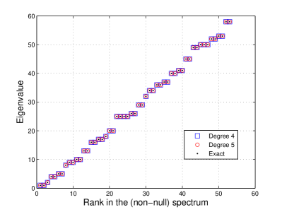
Figure 14: First non-null eigenvalues computed in the square for degrees 4 and 5.

Mode	Exact	Computed
(1,0)	1.00000	1.00001	1.00000	1.00000	1.00000	1.00000
(0,1)	1.00000	1.00005	1.00000	1.00000	1.00000	1.00000
(1,1)	2.00000	2.00016	2.00000	2.00000	2.00000	2.00000
(2,0)	4.00000	4.00396	4.00004	4.00000	4.00000	4.00000
(0,2)	4.00000	4.03882	4.00134	4.00002	4.00000	4.00000
(2,1)	5.00000	5.00395	5.00003	5.00000	5.00000	5.00000
(1,2)	5.00000	5.10164	5.00208	5.00002	5.00000	5.00000
(2,2)	8.00000	8.05454	7.99989	8.00001	8.00000	8.00000
(3,0)	9.00000	9.06255	9.00135	9.00001	9.00000	9.00000
(0,3)	9.00000	9.12399	9.02102	9.00057	9.00001	9.00000
(3,1)	10.0000	10.0614	10.0014	10.0000	10.0000	10.0000
(1,3)	10.0000	10.2361	10.0324	10.0007	10.0000	10.0000
(3,2)	13.0000	12.8159	13.0028	13.0000	13.0000	13.0000
(2,3)	13.0000	13.2002	13.0091	13.0004	13.0000	13.0000
(4,0)	16.0000	17.9413	16.0181	16.0002	16.0000	16.0000
(0,4)	16.0000	19.8934	16.2962	16.0076	16.0001	16.0000
(4,1)	17.0000	19.9586	17.0181	17.0002	17.0000	17.0000
(1,4)	17.0000	20.8937	18.0245	17.0092	17.0001	17.0000
(3,3)	18.0000	21.4707	18.7373	18.0008	18.0000	18.0000
(4,2)	20.0000	24.0689	20.0191	20.0002	20.0000	20.0000
(2,4)	20.0000	26.1844	21.6138	20.0056	20.0001	20.0000
d.o.f.		74	184	548	1852	6764
number of zeros		21	65	225	833	3201

Table 1: First non-null eigenvalues computed in the square for $p=3$.

Remark 6.1

We have also solved the previous test by the mixed formulations in [61], that make use of the full two-dimensional De Rham complex (57). The computed non-null eigenvalues are the same as for the plain formulation (67), while the zero eigenvalues are filtered with the mixed formulation. These results, that we do not present here for the sake of brevity, confirm that the construction of the De Rham complex with T-splines is correct.

6.2 Maxwell eigenproblem in the thick L-shaped domain

As a second test case, we solve the three-dimensional eigenvalue problem: Find $({\bf u},\omega)\in\,{\bf H}_{0}(\mathbf{curl};\Omega)\,\times\mathbb{R}$ such that

$$\int_{\Omega}\,{\bf curl}\,{\bf u}\cdot\,{\bf curl}\,\overline{\bf v}=\omega^{2}\int_{\Omega}{\bf u}\cdot\overline{\bf v}\quad\forall{\bf v}\in\,{\bf H}_{0}(\mathbf{curl};\Omega)\,,$$ (68)

in the thick L-shaped domain $\Omega=\Sigma\times(0,1)$, where $\Sigma=(-1,1)^{2}\setminus[-1,0]^{2}$. From [62], it is known that the reentrant edge introduces a singularity in the first eigenfunction, which only belongs to the space $H^{2/3-\varepsilon}(\Omega)$ for any $\varepsilon>0$.

It is well known that in order to recover the optimal convergence rate we need to suitably refine the mesh toward the reentrant edge, see e.g., [63] or [64]. Anisotropic elements need to be used in this case (see [21] for some theoretical background on the topic). We propose here a dyadic refinement based on T-splines.

For the geometry representation, the thick L-shaped domain is parametrized as the union of three cubic patches. Following Section 4.4, scalar fields in $X^{0}_{h}$ are only continuous at the interfaces between patches, and the fields in $X^{1}_{h}$, which are used in the discretization of (68), are only tangentially continuous at these interfaces (like for standard edge finite elements), but at least $C^{p-2}$ within patches.

The refinement is obtained via T-splines by dyadic partitioning of elements which are close to the reentrant edges [65, Ch. 4]. We perform the refinement first in an L-shaped two-dimensional section, and then propagate to the three-dimensional domain with a uniform mesh in the $z$-direction, as already explained in Section 5.4. The refinement is performed identically for every patch, in such a way that conformity can be ensured at the patch interfaces.

To construct the two-dimensional mesh, at each refinement step, and for every patch, we refine a small square region near the reentrant edge, subdividing each element into 4. Then some T-junction extensions are added, depending on the degree, to make the mesh analysis suitable, as defined in Section 5.2. For instance, in the example of Figure 15 we start with an $8\times 8$ mesh for each patch, which is drawn in black. At the first step we refine a region of $3\times 3$ elements on each patch. Since the degree is $p=4$, two-bay extensions must be added to make the mesh analysis suitable. The refined elements at this step are given by the blue lines. At the second refinement step, which is marked in red, we first refine a square region of $2\times 2$ elements, and again we add the two-bay extensions to make the mesh analysis suitable. Finally we remark that, since the dyadic partition and the definition of analysis suitable T-mesh depend on the degree, different meshes are used for different degrees.

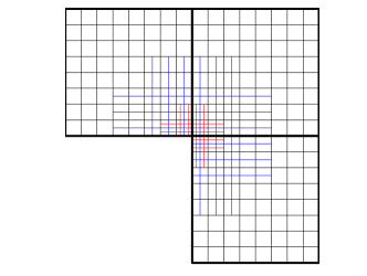
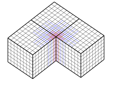
Figure 15: Example of a two-dimensional mesh in the L-shaped domain $\Sigma$, and its extension to the three-dimensional domain $\Omega=\Sigma\times(0,1)$ , for $p=4$.

The problem has been solved for degrees $4$ and $5$. In Tables 2 and 3 we present the first non-null computed eigenvalues in the three cases, and its comparison with the exact solution. In Figure 16 we display the convergence rate for the first eigenvalue, comparing the results obtained with T-splines and with a B-spline discretization of the same degree in the corresponding refined tensor-product dyadic mesh. As can be seen, with T-splines we obtain the same error with an important reduction in the number of the degrees of freedom.

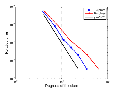
(a) Degree 4

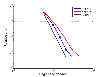
(b) Degree 5

Figure 16: Convergence of the first eigenvalue in the thick L-shaped domain.

Exact	Computed
9.63972384472	9.64482260735	9.64055367165	9.63986647533	9.63977706731	9.63974511214	9.63972731966
11.3452262252	11.3444193267	11.3450973393	11.3452056015	11.3452178503	11.3452228875	11.3452256921
13.4036357679	13.4036330719	13.4036359208	13.4036359870	13.4036357431	13.4036357654	13.4036357699
15.1972519265	15.1973643408	15.1973310163	15.1973301300	15.1972556440	15.1972524223	15.1972523662
19.5093282458	19.5144198480	19.5101576732	19.5094708082	19.5093814308	19.5093494993	19.5093317180
19.7392088022	19.7392474090	19.7392464705	19.7392464473	19.7392098765	19.7392090606	19.7392090522
19.7392088022	19.7392474115	19.7392464714	19.7392464480	19.7392098765	19.7392090617	19.7392090536
19.7392088022	19.7392854949	19.7392835833	19.7392835402	19.7392109156	19.7392092780	19.7392092574
21.2590837990	21.2591164396	21.2591199815	21.2591200740	21.2590848357	21.2590840605	21.2590840611
d.o.f.	4042	7126	11018	16162	22630	34894

Table 2: First non-null eigenvalues computed in the thick L-shaped domain for $p=4$.

Exact	Computed
9.63972384472	9.64328299807	9.64030443177	9.63981618307	9.63973902051	9.63973012738
11.3452262252	11.3446611860	11.3451346157	11.3452117088	11.3452238284	11.3452252153
13.4036357679	13.4036342774	13.4036357233	13.4036357613	13.4036357622	13.4036357630
15.1972519265	15.1972704673	15.1972555872	15.1972551905	15.1972551805	15.19725206245
19.5093282458	19.5128817631	19.5099083654	19.5094205444	19.5093433951	19.5093345086
19.7392088022	19.7392095886	19.7392095763	19.7392095758	19.7392095758	19.7392088273
19.7392088022	19.7392095886	19.7392095763	19.7392095758	19.7392095758	19.7392088273
19.7392088022	19.7392103678	19.7392103456	19.7392103444	19.7392103444	19.7392088514
21.2590837990	21.2590824582	21.2590845213	21.2590845754	21.2590845767	21.2590838179
d.o.f.	5891	9883	14827	20723	28105

Table 3: First non-null eigenvalues computed in the thick L-shaped domain for $p=5$.

6.3 Maxwell source problem in three quarters of the cylinder

For the third test case we consider the model source problem: Find ${\bf u}\in\,{\bf H}_{0,\Gamma_{D}}({\mathbf{curl}};\Omega)\,$ such that

$$\int_{\Omega}\,{\bf curl}\,{\bf u}\cdot\,{\bf curl}\,\overline{\bf v}+\int_{\Omega}{\bf u}\cdot\overline{\bf v}=\int_{\Omega}{\bf f}\cdot\overline{\bf v}\quad\forall{\bf v}\in\,{\bf H}_{0,\Gamma_{D}}({\mathbf{curl}};\Omega)\,,$$ (69)

where $\,{\bf H}_{0,\Gamma_{D}}({\mathbf{curl}};\Omega)\,$ is the set of functions with null tangential trace on $\Gamma_{D}\subset\partial\Omega$, i.e.,

$$\,{\bf H}_{0,\Gamma_{D}}({\mathbf{curl}};\Omega)\,:=\{{\bf v}\in\,{\bf H}({\mathbf{curl}};\Omega)\,:{\bf v}\times{\bf n}=\,{\bf 0}\text{ on }\Gamma_{D}\}.$$

The geometry $\Omega$ is three quarters of a cylinder of radius and length equal to one (see Figure 17), that in cylindrical coordinates is given by $\Omega=\{(r,\theta,z):0<r<1,\,0<\theta<\frac{3}{2}\pi,\,0<z<1\}$. We impose the null tangential component on $\Gamma_{D}=\{(r,\theta,z):\theta\in\{0,\frac{3}{2}\pi\}\}$, and the source term ${\bf f}$ is taken such that the exact solution is ${\bf u}=\,{\bf grad}\,(r^{2/3}\sin(2\theta/3)\sin(\pi z))$, i.e., it is singular in the first two directions, but it is regular in the $z$ direction, for which the local refinement of the previous test is well suited for this case.

As in the previous example, the domain is defined with three patches, and the discrete fields $X^{1}_{h}\subset\,{\bf H}({\mathbf{curl}};\Omega)\,$ are only tangentially continuous between them. The construction of the mesh in the parametric domain is identical to the one in the previous example: for each patch we first create a two-dimensional mesh locally refined towards the corner, and extend it to the three dimensional domain by tensor product. The mesh is then mapped to the physical domain, as can be seen in Figure 17.

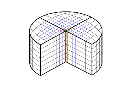
Figure 17: Example of a mesh for three quarters of the cylinder.

The problem is solved with T-splines of degree 3, and also with B-splines of the same degree in the corresponding tensor product mesh. The errors in ${\bf H}(\bf curl)$-norm for the two methods are compared in Figure 18. As in the previous example, with T-splines we are able to obtain results similar to those of B-splines with a reduction of the number of degrees of freedom.

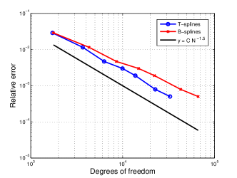
Figure 18: Comparison of the error for T-splines and B-splines.

6.4 Numerical simulation of a twisted waveguide

As the last numerical test we use T-splines to simulate the propagation of a singular mode in a waveguide with a twist. The configuration, which is presented in Figure 19(a), is the same given in [66, Ch. 8], changing the material discontinuity by a geometric inhomogeneity (the twist). The problem is solved in a waveguide with a twist of 90 degrees, with a section of three quarters of the circle of 2 cm radius, and for which we assume that the walls are perfect electrical conductors. We also assume that the waveguide extends to infinity without other inhomogeneities, and it is truncated by the planes $\Gamma_{1}$ and $\Gamma_{2}$ to obtain the computational domain, which consists of three different regions: a middle region where the waveguide is twisted (see Figure 19(a)), and two straight regions near the ports, to keep the inhomogeneity far enough from them, in such a way that only the dominant mode TE₁₀ can propagate without attenuation. The total length of the computational domain is 24 cm: 4 cm for each straight region, and 16 cm for the region with the twist. The frequency $\omega$ is taken equal to 32 GHz, and it is between the cutoff frequencies for the first mode (21 GHz) and the second mode (33.84 GHz).

Following [66], and working in the time harmonic regime at a given frequency $\omega$, the (complex-valued) electric field ${\bf E}\in\,{\bf H}_{0,\Gamma_{D}}({\mathbf{curl}};\Omega)\,$ is solution of the problem

$$\begin{array}[]{rcl}\displaystyle\int_{\Omega}(\,{\bf curl}\,{\bf E}\cdot\,{\bf curl}\,\overline{\bf G}-k^{2}{\bf E}\cdot\overline{\bf G})&+&\displaystyle\int_{\Gamma_{1}\cup\Gamma_{2}}{\rm i}\beta_{10}({\bf n}\times{\bf E})\cdot({\bf n}\times\overline{\bf G})=\\ &&\displaystyle 2{\rm i}\beta_{10}\,\int_{\Gamma_{1}}{\bf E}^{\rm inc}\cdot\overline{\bf G},\quad\forall{\bf G}\in\,{\bf H}_{0,\Gamma_{D}}({\mathbf{curl}};\Omega)\,,\end{array}$$ (70)

where $k=\sqrt{\omega^{2}\mu_{0}\varepsilon_{0}}$ with $\mu_{0}$ and $\varepsilon_{0}$ the magnetic permeability and electric permittivity of free space. The incident electric field ${\bf E}^{\rm inc}$ at the port $\Gamma_{1}$, and the wavenumber of the first mode $\beta_{10}$ are defined as

$${\bf E}^{\rm inc}(x,y,z)={\bf e}_{10}(x,y)e^{-{\rm i}\beta_{10}z}, \beta_{10}=\sqrt{k^{2}-k_{10}^{2}}.$$

In the case of waveguides of rectangular or circular section, the value of the constant $k_{10}$ and the mode ${\bf e}_{10}$ are known. In the general case, they can be obtained by solving a 2D eigenvalue problem on the port $\Gamma_{1}$, which consists on finding the minimum eigenvalue $k_{10}\in\mathbb{R}$, and its associated eigenvector ${\bf e}_{10}\in{\bf H}_{0}(\,{\rm rot}\,;\Gamma_{1})$, such that

$$\int_{\Gamma_{1}}\,{\rm rot}\,{\bf e}_{10}\,\,{\rm rot}\,\overline{\bf v}=k_{10}^{2}\int_{\Gamma_{1}}{\bf e}_{10}\cdot{\bf v}\quad\forall{\bf v}\in{\bf H}_{0}(\,{\rm rot}\,;\Gamma_{1}).$$ (71)

The electric field ${\bf E}$ in equation (70) is discretized with T-splines of degree 3, using the approach already explained in Section 5.4. The two-dimensional T-mesh for the section is built as in the previous examples, and in the $z$ direction we use one element for each straight region near the ports, and 4 elements along the twist, for a total of 7936 degrees of freedom. For the solution of the 2D problem (71), it is enough to restrict a field in $\,{\bf H}({\mathbf{curl}};\Omega)\,$ to its tangential components on the port $\Gamma_{1}$, which in practice is equivalent to solve with two-dimensional T-splines.

The magnitude of the real part of the computed solution ${\bf E}$ is shown in Figure 19(b), which shows that the mode is correctly propagated. Finally, we also compute the reflection and transmission coefficients, given by the equations

$$R=\frac{e^{-{\rm i}\beta z_{1}}\int_{\Gamma_{1}}{\bf E}\cdot{\bf e}_{10}}{\int_{\Gamma_{1}}{\bf e}_{10}\cdot{\bf e}_{10}}-e^{-2{\rm i}\beta z_{1}},\qquad T=\frac{e^{{\rm i}\beta z_{2}}\int_{\Gamma_{1}}{\bf E}\cdot{\bf e}_{10}}{\int_{\Gamma_{1}}{\bf e}_{10}\cdot{\bf e}_{10}}-e^{-2{\rm i}\beta z_{2}},$$

and we obtain the values $|R|=0.0025$ and $|T|=0.9998$, which confirms that the twist does not affect the propagation of the mode, as expected.

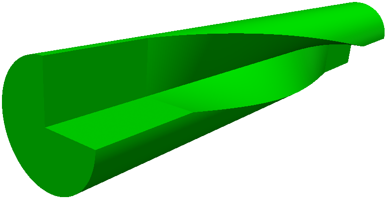
(a) Geometry of the waveguide

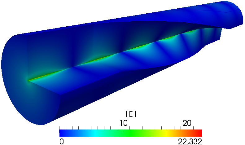
(b) Real part of the computed electric field

Figure 19: Geometry of the waveguide and real part of the computed electric field.

References

- [1] R. Hiptmair, Finite elements in computational electromagnetism, Acta Numer. 11 (2002) 237–339.
- [2] D. N. Arnold, R. S. Falk, R. Winther, Finite element exterior calculus, homological techniques, and applications, Acta Numer. 15 (2006) 1–155.
- [3] D. Boffi, Finite element approximation of eigenvalue problems, Acta Numer. 19 (2010) 1–120.
- [4] D. Boffi, P. Fernandes, L. Gastaldi, I. Perugia, Computational models of electromagnetic resonators: analysis of edge element approximation, SIAM J. Numer. Anal. 36 (4) (1999) 1264–1290 (electronic).
- [5] D. Braess, J. Schöberl, Equilibrated residual error estimator for edge elements, Math. Comp. 77 (262) (2008) 651–672.
- [6] L. Piegl, W. Tiller, The Nurbs Book, Springer-Verlag, New York, 1997.
- [7] T. Sederberg, J. Zheng, A. Bakenov, A. Nasri, T-splines and T-NURCCSs, ACM Trans. Graph. 22 (3) (2003) 477–484.
- [8] J. A. Cottrell, T. J. R. Hughes, Y. Bazilevs, Isogeometric Analysis: toward integration of CAD and FEA, John Wiley & Sons, 2009.
- [9] T. J. R. Hughes, J. A. Cottrell, Y. Bazilevs, Isogeometric analysis: CAD, finite elements, NURBS, exact geometry and mesh refinement, Comput. Methods Appl. Mech. Engrg. 194 (39-41) (2005) 4135–4195.
- [10] Y. Bazilevs, V. M. Calo, T. J. R. Hughes, Y. Zhang, Isogeometric fluid-structure interaction: theory, algorithms, and computations, Comput. Mech. 43 (1) (2008) 3–37.
- [11] J. A. Cottrell, A. Reali, Y. Bazilevs, T. J. R. Hughes, Isogeometric analysis of structural vibrations, Comput. Methods Appl. Mech. Engrg. 195 (41-43) (2006) 5257–5296.
- [12] R. Echter, M. Bischoff, Numerical efficiency, locking and unlocking of NURBS finite elements, Computer Methods in Applied Mechanics and Engineering 199 (5–8) (2010) 374 – 382.
- [13] S. Lipton, J. A. Evans, Y. Bazilevs, T. Elguedj, T. J. R. Hughes, Robustness of isogeometric structural discretizations under severe mesh distortion, Comput. Methods Appl. Mech. Engrg. 199 (5-8) (2010) 357 – 373.
- [14] E. Rank, M. Ruess, S. Kollmannsberger, D. Schillinger, A. Düster, Geometric modeling, isogeometric analysis and the finite cell method, Comput. Methods Appl. Mech. Engrg. (2012) doi: http://dx.doi.org/10.1016/j.cma.2012.05.022.
- [15] L. De Lorenzis, İ. Temizer, P. Wriggers, G. Zavarise, A large deformation frictional contact formulation using NURBS-based isogeometric analysis, Internat. J. Numer. Methods Engrg. 87 (13) (2011) 1278–1300.
- [16] T. Dokken, E. Quak, V. Skytt, Requirements from Isogeometric Analysis for changes in product design ontologies, in: Proceedings of the FOCUS K3D Conference on Semantic 3D Media and Content (INRIA Sophia Antipolis - Méditerranée, 2010), IMATI-CNR, Genova, Italy, 2010, pp. 11–15.
- [17] T. Martin, E. Cohen, R. Kirby, Volumetric parameterization and trivariate b-spline fitting using harmonic functions, Computer Aided Geometric Design 26 (6) (2009) 648 – 664, Solid and Physical Modeling 2008, ACM Symposium on Solid and Physical Modeling and Applications.
- [18] E. Cohen, T. Martin, R. M. Kirby, T. Lyche, R. F. Riesenfeld, Analysis-aware modeling: understanding quality considerations in modeling for isogeometric analysis, Comput. Methods Appl. Mech. Engrg. 199 (5-8) (2010) 334–356.
- [19] Y. Zhang, W. Wang, T. J. R. Hughes, Solid T-spline construction from boundary representations for genus-zero geometry, Comput. Methods Appl. Mech. Engrg. (2012) (to appear).
- [20] Y. Bazilevs, L. Beirão da Veiga, J. A. Cottrell, T. J. R. Hughes, G. Sangalli, Isogeometric analysis: approximation, stability and error estimates for -refined meshes, Math. Models Methods Appl. Sci. 16 (7) (2006) 1031–1090.
- [21] L. Beirão da Veiga, A. Buffa, D. Cho, G. Sangalli, Anisotropic NURBS approximation in Isogeometric Analysis, Comput. Methods Appl. Mech. Engrg. 209-212 (2012) 1–11.
- [22] A. Buffa, J. Rivas, G. Sangalli, R. Vázquez, Isogeometric discrete differential forms in three dimensions, SIAM J. Numer. Anal. 49 (2) (2011) 818–844.
- [23] J. A. Evans, Y. Bazilevs, I. Babuska, T. J. R. Hughes, N-widths, sup-infs, and optimality ratios for the k-version of the isogeometric finite element method, Comput. Methods Appl. Mech. Engrg. 198 (21-26) (2009) 1726–1741.
- [24] A.-V. Vuong, C. Giannelli, B. Jüttler, B. Simeon, A hierarchical approach to adaptive local refinement in isogeometric analysis, Comput. Methods Appl. Mech. Engrg. 200 (49-52) (2011) 3554–3567.
- [25] L. Beirão da Veiga, D. Cho, L. Pavarino, S. Scacchi, Overlapping Schwarz methods for Isogeometric Analysis, SIAM J. Numer. Anal. 50 (3) (2012) 1394–1416.
- [26] S. K. Kleiss, C. Pechstein, B. Jüttler, S. Tomar, IETI-Isogeometric Tearing and Interconnecting, Comput. Methods Appl. Mech. Engrg. (2012) (accepted for publication).
- [27] A. Buffa, G. Sangalli, R. Vázquez, Isogeometric analysis in electromagnetics: B-splines approximation, Comput. Methods Appl. Mech. Engrg. 199 (17-20) (2010) 1143 – 1152.
- [28] A. Ratnani, E. Sonnendrücker, An arbitrary high-order spline finite element solver for the time domain Maxwell equations, J. Sci. Comput. 51 (2012) 87–106.
- [29] E. Cohen, R. Riesenfeld, G. Elber, Geometric modeling with splines: an introduction, Vol. 1, AK Peters Wellesley, MA, 2001.
- [30] C. de Boor, A practical guide to splines, revised Edition, Vol. 27 of Applied Mathematical Sciences, Springer-Verlag, New York, 2001.
- [31] T. Sederberg, D. Cardon, G. Finnigan, N. North, J. Zheng, T. Lyche, T-spline simplication and local refinement, ACM Trans. Graph. 23 (3) (2004) 276–283.
- [32] Y. Bazilevs, V. Calo, J. A. Cottrell, J. A. Evans, T. J. R. Hughes, S. Lipton, M. Scott, T. Sederberg, Isogeometric analysis using T-splines, Comput. Methods Appl. Mech. Engrg. 199 (5-8) (2010) 229 – 263.
- [33] A. Buffa, D. Cho, G. Sangalli, Linear independence of the T-spline blending functions associated with some particular T-meshes, Comput. Methods Appl. Mech. Engrg. 199 (23–24) (2010) 1437–1445.
- [34] M. Scott, X. Li, T. Sederberg, T. J. R. Hughes, Local refinement of analysis-suitable T-splines, Comput. Methods Appl. Mech. Engrg. 213 - 216 (2012) 206 – 222.
- [35] W. Wang, Y. Zhang, M. Scott, T. J. R. Hughes, Converting an unstructured quadrilateral mesh to a standard T-spline surface, Comput. Mech. 48 (4) (2011) 477–498.
- [36] L. Beirão da Veiga, A. Buffa, D. Cho, G. Sangalli, IsoGeometric analysis using T-splines on two-patch geometries, Comput. Methods Appl. Mech. Engrg. 200 (21-22) (2011) 1787–1803.
- [37] X. Li, J. Zheng, T. Sederberg, T. Hughes, M. Scott, On linear independence of T-spline blending functions, Comput. Aided Geom. Design 29 (1) (2012) 63 – 76.
- [38] L. Beirão da Veiga, A. Buffa, D. Cho, G. Sangalli, Analysis-Suitable T-splines are Dual-Compatible, Comput. Methods Appl. Mech. Engrg. (2012) (to appear).
- [39] M. Scott, T-splines as a design-through-analysis technology, Ph.D. thesis, The University of Texas at Austin (2011).
- [40] D. N. Arnold, R. S. Falk, R. Winther, Finite element exterior calculus: from Hodge theory to numerical stability, Bull. Amer. Math. Soc. (N.S.) 47 (2) (2010) 281–354.
- [41] A. Buffa, C. de Falco, G. Sangalli, Isogeometric Analysis: stable elements for the 2D Stokes equation, Internat. J. Numer. Methods Fluids 65 (11-12) (2011) 1407–1422.
- [42] J. A. Evans, T. J. R. Hughes, Discrete spectrum analyses for various mixed discretizations of the Stokes eigenproblem, Computational Mechanics (2012) (accepted for publication).
- [43] J. A. Evans, T. J. R. Hughes, Isogeometric divergence-conforming B-splines for the Darcy-Stokes-Brinkman equations., Math. Models Methods Appl. Sci. (2012) (accepted for publication)doi:10.1142/S0218202512500583.
- [44] J. A. Evans, T. J. R. Hughes, Isogeometric divergence-conforming B-splines for the Steady Navier-Stokes Equations, Tech. Rep. 12-15, ICES, UT Austin (2012).
- [45] J. A. Evans, T. J. R. Hughes, Isogeometric divergence-conforming B-splines for the Unsteady Navier-Stokes Equations, Tech. Rep. 12-16, ICES, UT Austin (2012).
- [46] P. Monk, Finite Element Methods for Maxwell’s Equations, Oxford University Press, Oxford, 2003.
- [47] L. Beirão da Veiga, A. Buffa, G. Sangalli, R. Vázquez, Analysis-suitable T-splines of arbitrary degree: definition and properties, Tech. rep., IMATI-CNR (2012).
- [48] J.-C. Nédélec, Mixed finite elements in , Numer. Math. 35 (1980) 315–341.
- [49] A. Buffa, S. H. Christiansen, A dual finite element complex on the barycentric refinement, Math. Comp. 76 (260) (2007) 1743–1769 (electronic).
- [50] H. De Gersem, M. Wilke, M. Clemens, T. Weiland, Efficient modelling techniques for complicated boundary conditions applied to structured grids, COMPEL 23 (4) (2004) 904–912.
- [51] M. Clemens, P. Thoma, T. Weiland, U. van Rienen, Computational electromagnetic-field calculation with the finite-integration method, Surveys Math. Indust. 8 (3-4) (1999) 213–232.
- [52] R. Hiptmair, Discrete Hodge operators, Numer. Math. 90 (2) (2001) 265–289.
- [53] A. Bossavit, Discretization of electromagnetic problems: the “generalized finite differences” approach, in: Handbook of numerical analysis. Vol. XIII, Handb. Numer. Anal., XIII, North-Holland, Amsterdam, 2005, pp. 105–197.
- [54] X. Li, M. Scott, On the nesting behavior of T-splines, Tech. Rep. 11-13, ICES (2011).
- [55] M. Scott, M. Borden, C. Verhoosel, T. Sederberg, T. J. R. Hughes, Isogeometric finite element data structures based on Bézier extraction of T-splines, Internat. J. Numer. Methods Engrg. 88 (2) (2011) 126–156.
- [56] A. Bressan, T-splines characterization, in preparation.
- [57] B. Mourrain, On the dimension of spline spaces on planar T-meshes, Tech. rep., INRIA, http://hal.inria.fr/inria-00533187/en (2012).
- [58] X. Li, F. Chen, On the instability in the dimension of splines spaces over T-meshes, Comput. Aided Geom. Design 28 (7) (2011) 420–426.
- [59] R. Vázquez, A. Buffa, Isogeometric analysis for electromagnetic problems, Magnetics, IEEE Transactions on 46 (8) (2010) 3305 –3308.
- [60] C. de Falco, A. Reali, R. Vázquez, GeoPDEs: a research tool for Isogeometric Analysis of PDEs, Adv. Eng. Softw. 42 (12) (2011) 1020–1034.
- [61] D. Boffi, Approximation of eigenvalues in mixed form, discrete compactness property, and application to mixed finite elements, Comput. Methods Appl. Mech. Engrg. 196 (37-40) (2007) 3672–3681.
- [62] M. Costabel, M. Dauge, Singularities of electromagnetic fields in polyhedral domains, Arch. Ration. Mech. Anal. 151 (3) (2000) 221–276.
- [63] S. Nicaise, Edge elements on anisotropic meshes and approximation of the Maxwell equations, SIAM J. Numer. Anal. 39 (3) (2001) 784–816 (electronic).
- [64] A. Buffa, M. Costabel, M. Dauge, Algebraic convergence for anisotropic edge elements in polyhedral domains, Numer. Math. 101 (1) (2005) 29–65.
- [65] T. Apel, Anisotropic finite elements: local estimates and applications, Advances in Numerical Mathematics, B. G. Teubner, Stuttgart, 1999.
- [66] J. Jin, The finite element method in electromagnetics, 2nd Edition, Wiley-Interscience [John Wiley & Sons], New York, 2002.