QCD modified ghost scalar field dark energy models

Abstract

Within the framework of FRW cosmology, we study the QCD modified ghost scalar field models of dark energy in the presence of both interaction and viscosity. For a spatially non-flat FRW universe containing modified ghost dark energy (MGDE) and dark matter, we obtain the equation of state of MGDE, the deceleration parameter as well as a differential equation governing the MGDE density parameter. We also investigate the growth of structure formation for our model in a linear perturbation regime. Furthermore, we reconstruct both the dynamics and potentials of the quintessence, tachyon, K-essence and dilaton scalar field DE models according to the evolution of the MGDE density.

PACS numbers: 98.80.$-$k, 95.36.+x
Keywords: Cosmology, Dark energy

1 Introduction

Astronomical data from the supernova type Ia (SNeIa) [1, 2, 3, 4, 5], cosmic microwave background (CMB) [6, 7, 8], large scale structure (LSS) [9, 10, 11], baryon acoustic oscillations (BAO) [12] and weak lensing [13] indicate that expansion of the universe is speeding up rather than decelerating. It is believed that the present accelerated expansion is driven by gravitationally repulsive dominant energy component known as “dark energy” (DE). Although the nature of DE remains a mystery, various models of DE have been proposed in the literature (for review see [14, 15, 16]). Theoretically, the simplest candidate for such a component is a small positive cosmological constant, but it suffers the difficulties associated with the fine tuning and the cosmic coincidence problems [17].

More recently, a new DE model called ghost DE (GDE) has been motivated from the Veneziano ghost of choromodynamics (QCD) [18, 19, 20]. The Veneziano ghost is required to exist for the resolution of the $U(1)_{A}$ problem in low energy effective theory of QCD. The ghosts make no contribution in the flat Minkowski space, but once they are in the curved space or time-dependent background such as our Friedmann-Robertson-Walker (FRW) universe, the cancelation of their contribution to the vacuum energy is off-set, leaving a small energy density $\sim\Lambda^{3}_{\rm QCD}H$, where $H$ is the Hubble parameter and $\Lambda_{\rm QCD}\sim 100$ MeV is the QCD mass scale [21, 22, 23, 24, 25]. This small contribution can play an important role in the evolutionary behavior of the universe. For instance, taking $H\sim 10^{-33}$eV at the present, $\Lambda^{3}_{\rm QCD}H$ gives the right order of observed magnitude of the DE density. This coincidence is remarkable and implies that the GDE model gets rid of fine tuning problem [18, 19, 20]. In addition, the appearance of the QCD scale could be relevant for a solution to the cosmic coincidence problem, as it may be the scale at which dark matter (DM) forms [26]. The other advantage of the GDE with respect to other DE models include the fact that it can be completely explained within the standard model and general relativity (GR), without recourse to any new field, new degree(s) of freedom, new symmetries or modifications of GR. It is worth to note that the GDE model does not violate unitarity, causality, gauge invariance and other important features of renormalizable quantum field theory, as advocated in [27, 28, 29].

The ordinary GDE density is given by [18, 19, 20]

$$\rho_{D}=\alpha H,$$ (1)

where $\alpha$ is a constant with dimension $[{\rm energy}]^{3}$, and roughly of order of $\Lambda_{\rm QCD}^{3}$. This new kind of DE model has got a lot of enthusiasm recently in the literature [30, 31, 32, 33, 34, 35, 36, 37, 38, 39, 40]. Although the ordinary GDE model is consistent with the observational data, it suffers from the difficulty to describe the early evolution of the universe. This motivated Cai et al. [41] to introduce the modified GDE (MGDE) density as

$$\rho_{D}=\alpha H+\beta H^{2},$$ (2)

where the constant $\alpha$ is same as that defined in the ordinary GDE and $\beta$ is another constant with dimension $[{\rm energy}]^{2}$. Note that the Veneziano ghost field in QCD is originated from the vacuum energy of quantum fields which is of the form $H+{\mathcal{O}}(H^{2})$ [42]. However, in the ordinary GDE model, only the leading term $H$ has been considered. Although the subleading term $H^{2}$ is too small and cannot drive the universe to accelerating expansion, Cai et al. [41] showed that this term can play an important role in the early evolution of the universe, acting as an early DE. Using the joint analysis of the astronomical data, Cai et al. [41] found that the subleading term $H^{2}$ of the DE density–the early DE–could have a fraction energy density around $10\%$. Indeed, the term proportional to $H^{2}$ is related to the difference between the vacuum energies in Minkowski space and in a FRW universe [43, 44]. On the other hand, the vacuum energy difference from the Veneziano ghost field introduced in order to solve the so-called $U(1)_{A}$ problem in QCD has the exact form $\alpha H+\beta H^{2}$, where $\alpha\sim\Lambda_{\rm QCD}^{3}\sim(100~{}{\rm MeV})^{3}$. For other motivations to consider this form of DE, see again [41], where the MGDE model has been fitted with current observational data including SNeIa, BAO, CMB, big bang nucleosynthesis (BBN), Hubble parameter and growth rate of matter perturbation in order to get some constraints on the model parameters. It was found that the MGDE model, without having the two fundamental cosmological puzzles, like the $\Lambda$CDM fit the astronomical data very well.

On the other hand, as is well known, an alternative proposal for DE is scalar field scenarios such as quintessence, tachyon, K-essence and dilaton (for review see [45] and references therein). The scalar field models are an effective description of an underlying theory of DE and can alleviate the fine tuning and cosmic coincidence problems [46]. Scalar fields naturally arise in particle physics including supersymmetric field theories and string/M theory. Therefore, scalar field is expected to reveal the dynamical mechanism and the nature of DE. Although fundamental theories such as string/M theory do provide a number of possible candidates for scalar fields, they do not uniquely predict their field $\phi$ and potential $V(\phi)$ [47]. Therefore it becomes meaningful to reconstruct both the dynamics and potentials of the scalar fields from some DE models such as holographic [48, 49, 50, 51, 52, 53, 54], agegraphic [55, 56, 57, 58] and ordinary ghost [38, 39, 40].

Describing the DE model in a scalar field framework provides a more fundamental representation of the dark component. This motivates us to establish different scalar field models according to evolutionary behavior of the MGDE scenario. To do so, in section 2 we investigate the MGDE in a spatially non-flat FRW universe. In section 3 we study the growth of structure formation in our model. In section 4 we reconstruct both the dynamics $\phi$ and potentials $V(\phi)$ of the quintessence, tachyon, K-essence and dilaton scalar field models of DE according to the evolution of MGDE density. Section 5 is devoted to conclusions.

2 The Veneziano MGDE and DM

Within the framework of Einstein gravity, we consider a spatially non-flat FRW universe filled with MGDE density $\rho_{D}$ and DM energy density $\rho_{\rm m}$. Therefore, the first Friedmann equation reads

$$H^{2}+\frac{k}{a^{2}}=\frac{1}{3M_{P}^{2}}~{}(\rho_{D}+\rho_{\rm m}),$$ (3)

where the scalar curvature $k=0,1,-1$ denote a flat, closed and open FRW universe, respectively. Also $M_{P}=(8\pi G)^{-1/2}$ is the reduced Planck mass.

Using the fractional energy densities

$$\Omega_{\rm m}=\frac{\rho_{\rm m}}{\rho_{\rm cr}}=\frac{\rho_{\rm m}}{3M_{P}^{2}H^{2}},~{}~{}~{}\Omega_{D}=\frac{\rho_{D}}{\rho_{\rm cr}}=\frac{\rho_{D}}{3M_{P}^{2}H^{2}},~{}~{}~{}\Omega_{k}=\frac{k}{a^{2}H^{2}},$$ (4)

the Friedmann equation (3) can be rewritten as

$$1+\Omega_{k}=\Omega_{D}+\Omega_{\rm m}.$$ (5)

Substituting Eq. (2) into the middle relation of Eq. (4) gives

$$\Omega_{D}=\frac{\alpha}{3M^{2}_{P}H}+1-\gamma,$$ (6)

where

$$\gamma=1-\frac{\beta}{3M_{P}^{2}}.$$ (7)

Using Eq. (6), the curvature energy density parameter takes the form

$$\Omega_{k}=\frac{\Omega_{k_{0}}}{(\Omega_{D_{0}}+\gamma-1)^{2}}\left(\frac{\Omega_{D}+\gamma-1}{a}\right)^{2},$$ (8)

where we take $a_{0}=1$ for the present time and the subscript “0” denotes the present value of a quantity.

Following the observational evidences we extend our study to the case in which the MGDE has a bulk viscosity property [59, 60, 61] and also interact with DM [62, 63]. It is well known that in the framework of FRW metric, the shear viscosity has no contribution in the energy momentum tensor, and the bulk viscosity behaves like an effective pressure. Because, the CMB does not indicate significant anisotropy due to shear viscosity and only bulk viscosity is taken into account for the fluids in the cosmological context [64]. In viscous cosmology, shear and bulk viscosities arise in relation to space anisotropy and isotropy, respectively. It was also pointed out that the bulk viscosity can play a significant role in the formation of the LSS of the universe [65]. It can also alleviate several cosmological puzzles like age problem and cosmic coincidence problem [66, 67, 68, 69].

The interaction between DE and DM can be detected in the formation of LSS. It was suggested that the dynamical equilibrium of collapsed structures such as galaxy clusters would be modified due to the coupling between DE and DM. The recent observational evidence provided by the galaxy cluster Abell A586 supports the interaction between DE and DM [70]. The other observational signatures on the dark sectors’ mutual interaction can be found in the probes of the cosmic expansion history by using the SNeIa, BAO and CMB shift data [71].

In the presence of bulk viscosity and interaction, the energy densities of MGDE and DM do not conserve separately and continuity equations take the forms

$$\dot{\rho}_{D}+3H(1+\omega_{D})\rho_{D}=9H^{2}\xi-Q,$$ (9)

$$\dot{\rho}_{\rm m}+3H\rho_{\rm m}=Q,$$ (10)

where $\omega_{D}=p_{D}/\rho_{D}$ is the equation of state (EoS) parameter of MGDE. Also $\xi=\epsilon H^{-1}\rho_{D}$ is the bulk viscosity coefficient with the viscosity constant $\epsilon$ [66, 67, 68, 69] and $Q=3b^{2}H(\rho_{D}+\rho_{\rm m})$ is the interaction term with the coupling constant $b^{2}$ [72]. This expression for the interaction term $Q$ was first introduced in the study of the suitable coupling between a quintessence scalar field and a pressureless cold DM field [73].

Taking time derivative of Eq. (3) and using Eqs. (4), (5), (9) and (10) one can get

$$\frac{\dot{H}}{H^{2}}=-\frac{3}{2}\left[1+\frac{\Omega_{k}}{3}+(\omega_{D}-3\epsilon)\Omega_{D}\right].$$ (11)

Taking time derivative of Eq. (2), using (11), and substituting the obtained result into Eq. (9) gives the EoS parameter of the interacting viscous MGDE as

$$\omega_{D}=\frac{1}{\Omega_{D}-\gamma-1}\left[1-\frac{\Omega_{k}}{3}+\frac{\gamma-1}{\Omega_{D}}\left(1+\frac{\Omega_{k}}{3}\right)+2b^{2}\left(\frac{1+\Omega_{k}}{\Omega_{D}}\right)\right]+3\epsilon.$$ (12)

For completeness, we give the deceleration parameter

$$q=-1-\frac{\dot{H}}{H^{2}},$$ (13)

which combined with the dimensionless density parameter $\Omega_{D}$ and the EoS parameter $\omega_{D}$ form a set of useful parameters for the description of the astrophysical observations. Replacing Eq. (12) into (11) gives

$$q=\frac{\gamma+2(\Omega_{D}-1)-\Omega_{k}+3b^{2}(1+\Omega_{k})}{\Omega_{D}-\gamma-1}.$$ (14)

Taking the derivative of Eq. (6) with respect to redshift $z=\frac{1}{a}-1$ and using Eqs. (11) and (12) gives

$$\frac{{\rm d}\Omega_{D}}{{\rm d}z}=-\left(\frac{3}{1+z}\right)\left(\frac{\Omega_{D}+\gamma-1}{\Omega_{D}-\gamma-1}\right)\left[\Omega_{D}-1-\frac{\Omega_{k}}{3}+b^{2}(1+\Omega_{k})\right].$$ (15)

Note that Eqs. (14) and (15) show that both the deceleration and MGDE density parameters are independent of viscosity constant. The viscosity appeared only in the dynamical EoS parameter of MGDE, Eq. (12).

We solve the differential equation governing the MGDE density parameter, Eq. (15), numerically. In Fig. 1, variation of the MGDE density parameter $\Omega_{D}$ versus redshift $z=\frac{1}{a}-1$ for different coupling constants $b^{2}$ is plotted. Figure 1 shows that: i) for a given $b^{2}$, $\Omega_{D}$ increases during history of the universe. ii) At early and late times, $\Omega_{D}$ increases and decreases, respectively, with increasing $b^{2}$.

In Fig. 2 we plot the evolutionary behavior of the deceleration parameter, Eq. (14), for different $b^{2}$. Figure 2 presents that: i) the universe transitions from a matter dominated epoch at early times to the de Sitter phase, i.e. $q=-1$, in the future, as expected. The result for $b^{2}=0$ is in agreement with that obtained by [41]. ii) For $b^{2}=0.0$, $0.02$ and $0.04$ at $z=0.75$, $0.91$ and $1.10$, respectively, we have a cosmic deceleration $q>0$ to acceleration $q<0$ transition which is compatible with the observations [74]. iii) For a given $z$, although $q$ decreases with increasing $b^{2}$, in the far future $q$ becomes independent of $b^{2}$.

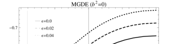
Figure 4: Same as Fig. 3 for different viscosity constants $\epsilon$ with $b^{2}=0$.

The variation of the EoS parameter of interacting viscous MGDE, Eq. (12), for different coupling $b^{2}$ and viscosity $\epsilon$ constants is plotted in Figs. 3, 4 and 5. Figures 3 and 4 illustrate that: i) in the absence of viscosity ($\epsilon=0$), $\omega_{D}(z)$ varies from the quintessence phases ($\omega_{D}>-1$) to the phantom regime ($\omega_{D}<-1$). ii) In the absence of interaction ($b^{2}=0$), $\omega_{D}(z)$ varies from $\omega_{D}>-1$ to $\omega_{D}=-1$, which is similar to the freezing quintessence model [75]. iii) For a given $z$, $\omega_{D}$ decreases and increases with increasing $b^{2}$ and $\epsilon$, respectively. Note that the result for $b^{2}=\epsilon=0$ is in accordance with that obtained by [41]. Figures 5 shows that the interaction and viscosity have opposite effects on $\omega_{D}$.

3 The growth of structure formation

Here we investigate the growth rate of matter in the presence of interaction between viscous MGDE and DM. Following [76], the structure formation takes place in the Newtonian regime. Hence, the equations of motion containing the Euler and Poisson equations for DM in the non-relativistic approximation reduce to

$$\frac{\partial{\mathbf{v}}}{\partial t}+({\mathbf{v}}.\nabla){\mathbf{v}}=-\frac{\nabla p_{\rm m}}{\rho_{\rm m}}-\nabla\phi,$$ (16)

$$\nabla^{2}\phi=4\pi G\rho_{\rm m},$$ (17)

where ${\mathbf{v}}$ and $\phi$ are the velocity of DM and gravitational potential, respectively. According to the linear perturbation theory [76], substituting the perturbations

$${\mathbf{v}}\rightarrow{\mathbf{v}}+\delta{\mathbf{v}},~{}~{}~{}p_{\rm m}\rightarrow p_{\rm m}+\delta p_{\rm m},~{}~{}~{}\rho_{\rm m}\rightarrow\rho_{\rm m}+\delta\rho_{\rm m},~{}~{}~{}\phi\rightarrow\phi+\delta\phi,$$ (18)

into Eqs. (16) and (17) and retaining only first order corrections to the background variable, one can obtain

$$\delta\dot{H}=-2H\delta H-\frac{4\pi G}{3}\delta\rho_{\rm m},$$ (19)

where we have used $\nabla.{\mathbf{v}}=3H$ and set $v_{s}^{2}=0$ for the pressureless DM ($p_{\rm m}=0$).

Now we generalize the linear perturbation formalism introduced in [76] to the case of interaction between viscous MGDE and DM. Note that Eq. (19) still holds in the presence of interaction and viscosity. Because the bulk viscous coefficient $\epsilon$ and the coupling constant of interaction term $b^{2}$ only appear in the continuity Eqs. (9) and (10).

From Eqs. (2) and (10), we have

$$\dot{\rho}_{\rm m}+3H\rho_{\rm m}=3b^{2}H(\alpha H+\beta H^{2}+\rho_{\rm m}).$$ (20)

Substituting the perturbations $\rho_{\rm m}\rightarrow\rho_{\rm m}+\delta\rho_{\rm m}$ and $H\rightarrow H+\delta H$ into the above relation yields the density perturbation equation for DM as

$$\delta\dot{\rho}_{\rm m}+3H(1-b^{2})\delta\rho_{\rm m}=\left[\frac{\rho_{\rm m}}{H}+3b^{2}(\alpha H+2\beta H^{2})\right]\delta H.$$ (21)

In terms of the DM density contrast $\delta_{\rm m}=\delta\rho_{\rm m}/\rho_{\rm m}$, Eq. (21) can be rewritten for $\delta H$ as

$$\delta H=\frac{\dot{\delta}_{\rm m}+\frac{3b^{2}}{\rho_{\rm m}}(\alpha H^{2}+\beta H^{3})\delta_{\rm m}}{-3(1-b^{2})+\frac{3b^{2}}{\rho_{\rm m}}(2\alpha H+3\beta H^{2})}.$$ (22)

Taking the time derivative of Eq. (22) gives

$$\delta\dot{H}=\frac{{\rm I}}{3\left[1-2b^{2}\Big{(}1+\frac{2\alpha H+3\beta H^{2}}{\rho_{\rm m}}\Big{)}\right]},$$ (23)

where

$${\rm I} = \left[b^{2}\left(1+\frac{2\alpha H+3\beta H^{2}}{\rho_{\rm m}}\right)-1\right]\ddot{\delta}_{\rm m}$$ (24)

$$+ \frac{b^{2}}{\rho_{\rm m}}\left[-7\alpha H^{2}-6\beta H^{3}+\frac{8\pi G}{3}\rho_{\rm m}(\alpha+3\beta H)\right]\dot{\delta}_{\rm m}$$

$$+ \frac{b^{2}}{\rho_{\rm m}}\left[-3\alpha H^{3}+4\pi G\rho_{\rm m}\Big{(}2\alpha H+3\beta H^{2}\Big{)}\right]\delta_{\rm m},$$

and from Eq. (19) we have used $\dot{H}=-H^{2}-4\pi G\rho_{\rm m}/3$. We also have neglected the terms higher than ${\mathcal{O}}(b^{2})$. Using the latest observations (golden SNeIa, the shift parameter of CMB and the BAO) and combining them with the lookback time data we have that $b^{2}$ could be as large as 0.2 (see [77]) although a value of $b^{2}<0.04$ is favored.

Inserting Eqs. (22) and (23) into (19) and using $\delta\rho_{\rm m}=\rho_{\rm m}\delta_{\rm m}$, one can get the evolution equation for the dimensionless DM density perturbation $\delta_{\rm m}$ as

$$~{}~{}\left\{1-b^{2}\left(1+\frac{2\alpha H+3\beta H^{2}}{\rho_{\rm m}}\right)\right\}\ddot{\delta}_{\rm m}$$

$$+\left\{2H+b^{2}\left(\frac{3\alpha H^{2}}{\rho_{\rm m}}-\frac{8\pi G}{3}(\alpha+3\beta H)-2H\right)\right\}\dot{\delta}_{\rm m}$$

$$-\left\{4\pi G\rho_{\rm m}-b^{2}\left[3H^{3}\left(\frac{3\alpha+2\beta H}{\rho_{\rm m}}\right)+4\pi G\Big{(}2\alpha H+3\beta H^{2}+2\rho_{\rm m}\Big{)}\right]\right\}\delta_{\rm m}=0.$$ (25)

Note that the viscosity constant $\epsilon$ does not appear in Eq. (25). This comes back to the fact that in our model, the DM has not the viscosity properties (see Eq. 10) and due to choosing a specific form for the bulk viscosity coefficient $\xi=\epsilon H^{-1}\rho_{D}$ in Eq. (9), the viscosity constant $\epsilon$ does not affect $\delta_{\rm m}$ in our model.

In the absence of interaction, i.e. $b^{2}=0$, Eq. (25) recovers the well known relation given by [76]

$$\ddot{\delta}_{\rm m}+2H\dot{\delta}_{\rm m}-4\pi G\rho_{\rm m}\delta_{\rm m}=0.$$ (26)

Using the following definitions

$$\bar{\ddot{\delta}}_{\rm m}=\ddot{\delta}_{\rm m}/H_{0}^{2},~{}~{}~{}\bar{\dot{\delta}}_{\rm m}=\dot{\delta}_{\rm m}/H_{0},~{}~{}~{}\bar{H}=H/H_{0},~{}~{}~{}\bar{\alpha}=\frac{\alpha}{3M_{P}^{2}H_{0}},$$ (27)

one can rewrite Eq. (25) in dimensionless form as

$${\mathcal{J}}_{1}\bar{\ddot{\delta}}_{\rm m}+{\mathcal{J}}_{2}\bar{\dot{\delta}}_{\rm m}+{\mathcal{J}}_{3}\delta_{\rm m}=0,$$ (28)

where

$${\mathcal{J}}_{1}=1-b^{2}\left[1+\frac{2\bar{\alpha}/\bar{H}+3(1-\gamma)}{\Omega_{\rm m}}\right],$$ (29)

$${\mathcal{J}}_{2}=2\bar{H}+b^{2}\left[\bar{\alpha}\left(\frac{3}{\Omega_{\rm m}}-1\right)+(3\gamma-5)\bar{H}\right],$$ (30)

$${\mathcal{J}}_{3}=-\frac{3}{2}\Omega_{\rm m}\bar{H}^{2}+3b^{2}\bar{H}\left[\left(\frac{3\bar{\alpha}+2(1-\gamma)\bar{H}}{\Omega_{\rm m}}\right)+\bar{\alpha}+\frac{3}{2}(1-\gamma)\bar{H}+\Omega_{\rm m}\bar{H}\right].$$ (31)

In terms of the growth factor $f$ defined as [76]

$$f(z)=\frac{{\rm d}\ln\delta_{\rm m}}{{\rm d}\ln a}=-(1+z)\frac{{\rm d}\ln\delta_{\rm m}}{{\rm d}z},$$ (32)

equation (28) can be rewritten as

$$-(1+z)\bar{H}^{2}\frac{{\rm d}f}{{\rm d}z}+\bar{H}\left[-(1+z)\frac{{\rm d}\bar{H}}{{\rm d}z}+\bar{H}f+\left(\frac{{\mathcal{J}}_{2}}{{\mathcal{J}}_{1}}\right)\right]f+\left(\frac{{\mathcal{J}}_{3}}{{\mathcal{J}}_{1}}\right)=0.$$ (33)

Note that for the matter dominated universe, i.e. $H^{2}=\rho_{\rm m}/3M_{P}^{2}$, solution of Eq. (26) yields $\delta_{\rm m}=a$. In this case, Eq. (32) gives the growth factor $f=1$.

In general, the differential equation (33) has no analytical solution. Hence, we need to solve it numerically. To do so, we first need to know the dimensionless Hubble parameter $\bar{H}(z)$. From Eq. (6) and last relation in Eq. (27) we obtain

$$\bar{H}(z)=\frac{\bar{\alpha}}{\Omega_{D}(z)+\gamma-1},$$ (34)

and

$$\bar{\alpha}=\Omega_{D_{0}}+\gamma-1.$$ (35)

Now with the help of $\Omega_{D}(z)$ plotted in Fig. 1 which has been already obtained by numerically solving Eq. (15), one can obtain the evolutionary behavior of the growth factor $f(z)$ of DM. In Fig. 6, variation of the growth factor $f(z)$ versus redshift for different coupling constants $b^{2}$ is plotted. Figure 6 shows that: i) for a given $b^{2}$, $f$ decreases during history of the universe. ii) For a given $z$, $f$ increases with increasing $b^{2}$. The result for $b^{2}=0$ is same as that obtained by [41].

Using Eq. (32), the dimensionless DM density perturbation $\delta_{\rm m}$ takes the form

$$\delta_{\rm m}(z)=\delta_{\rm m_{0}}\exp{\left[-\int_{0}^{z}\frac{f(z)}{1+z}~{}{\rm d}z\right]}.$$ (36)

In Fig. 7, we plot the evolutionary behavior of $\delta_{\rm m}(z)$ for different $b^{2}$. Figure 7 presents that: i) for a given $b^{2}$, $\delta_{\rm m}$ increases during history of the universe. ii) For a given $z$, $\delta_{\rm m}$ decreases with increasing $b^{2}$. This shows a suppression of structure growth relative to the non-interacting case. In the presence of interaction, there is less DM in the past (see Fig. 8), and this leads to a suppression in the growth of structure. This is in agreement with the result obtained by [78]. Note that the suppression is specific to the circumstance that the interacting and non-interacting cases are normalized to have the same parameters today, i.e. $\Omega_{\rm m_{0}}$ and $\delta_{\rm m_{0}}$.

4 Correspondence with scalar field models

Here, our aim is to investigate whether a minimally coupled scalar field with a specific action/Lagrangian can mimic the dynamics of the Veneziano MGDE model so that this model can be related to some fundamental theory (such as string/M theory), as it is for a scalar field. For this task, it is then meaningful to reconstruct the dynamics $\phi$ and potential $V(\phi)$ of a scalar field model possessing some significant features of the underlying theory of DE, such as the MGDE model. To do so and following the method proposed by [79], we establish a correspondence between the MGDE and various scalar field models by identifying their respective energy densities and equations of state and then reconstruct both the dynamics and potential of the field.

4.1 Quintessence MGDE

Quintessence is described by an ordinary time dependent and homogeneous scalar field $\phi$ which is minimally coupled to gravity, but with a particular potential $V(\phi)$ that leads to the accelerating universe. The action for quintessence is given by [45, 80, 81]

$$S=\int{\rm d}^{4}x\sqrt{-g}\left[-\frac{1}{2}g^{\mu\nu}\partial_{\mu}\phi\partial_{\nu}\phi-V(\phi)\right].$$ (37)

The energy density and pressure of the quintessence scalar field $\phi$ are as follows

$$\rho_{Q}=\frac{1}{2}\dot{\phi}^{2}+V(\phi),$$ (38)

$$p_{Q}=\frac{1}{2}\dot{\phi}^{2}-V(\phi).$$ (39)

The quintessence EoS parameter takes the form

$$\omega_{Q}=\frac{p_{Q}}{\rho_{Q}}=\frac{\dot{\phi}^{2}-2V(\phi)}{\dot{\phi}^{2}+2V(\phi)}.$$ (40)

Identifying Eq. (40) with the EoS parameter of interacting viscous MGDE (12), $\omega_{Q}=\omega_{D}$, and also equating Eq. (38) with (2), $\rho_{Q}=\rho_{D}$, one can get

$$V(\phi)=\frac{1}{2}(1-\omega_{D})\rho_{D},$$ (41)

$$\dot{\phi}^{2}=(1+\omega_{D})\rho_{D}.$$ (42)

Inserting Eqs. (2) and (12) into the above equations, one can get the quintessence potential and kinetic energy as

$$V(\phi)=\frac{\alpha^{2}\Omega_{D}}{6M^{2}_{P}(\Omega_{D}+\gamma-1)^{2}}\left[\frac{\Omega_{D}-\gamma-2+\frac{\Omega_{k}}{3}-\left(\frac{\gamma-1}{\Omega_{D}}\right)\left(1+\frac{\Omega_{k}}{3}\right)-2b^{2}\left(\frac{1+\Omega_{k}}{\Omega_{D}}\right)}{\Omega_{D}-\gamma-1}-3\epsilon\right],$$ (43)

$$\dot{\phi}^{2}=\frac{\alpha^{2}\Omega_{D}}{3M^{2}_{P}(\Omega_{D}+\gamma-1)^{2}}\left[\frac{\Omega_{D}-\gamma-\frac{\Omega_{k}}{3}+\left(\frac{\gamma-1}{\Omega_{D}}\right)\left(1+\frac{\Omega_{k}}{3}\right)+2b^{2}\left(\frac{1+\Omega_{k}}{\Omega_{D}}\right)}{\Omega_{D}-\gamma-1}+3\epsilon\right].$$ (44)

Integrating Eq. (44) with respect to $a$ and using (6) yields the modified ghost quintessence scalar field as

$$\phi(a)-\phi(a_{i})=\sqrt{3}~{}M_{P}\int^{a}_{a_{i}}\sqrt{\Omega_{D}}\left[\frac{\Omega_{D}-\gamma-\frac{\Omega_{k}}{3}+\left(\frac{\gamma-1}{\Omega_{D}}\right)\left(1+\frac{\Omega_{k}}{3}\right)+2b^{2}\left(\frac{1+\Omega_{k}}{\Omega_{D}}\right)}{\Omega_{D}-\gamma-1}+3\epsilon\right]^{\frac{1}{2}}~{}\frac{{\rm d}a}{a}.$$ (45)

The above integral cannot be taken analytically. But with the help of Eq. (8) and numerical solution of the differential equation (15) one can obtain the evolutionary behavior of the quintessence MGDE scalar field. In Figs. 9, 10 and 11 we plot the variation of scalar field, Eq. (45), versus redshift. Figures 9 and 10 present that: i) for a given $b^{2}$ or $\epsilon$, $\phi$ increases during history of the universe. ii) For a given $z$, $\phi$ decreases and increases with increasing $b^{2}$ and $\epsilon$, respectively. Figure 9 shows that for $b^{2}=0.0$, $0.02$ and $0.04$ at $z<-0.97$, $-0.57$ and $-0.41$, respectively, $\phi$ becomes pure imaginary, i.e. $\dot{\phi}^{2}<0$, and does not show itself in Fig. 9. For $\dot{\phi}^{2}<0$ the MGDE scalar field behaves as a phantom-type scalar field [82]. Figure 11 clarifies that interaction and viscosity have opposite effects on $\phi$. For $b^{2}=\epsilon$, the effect of viscosity is more than the interaction.

In Figs. 12, 13 and 14, the variation of quintessence MGDE potential, Eq. (43), versus redshift is presented for different $b^{2}$ and $\epsilon$. Figures 12 and 13 illustrate that: i) for a given $b^{2}$ or $\epsilon$, the quintessence MGDE potential $V(\phi)$ decreases during history of the universe. ii) For a given $z$, $V(\phi)$ increases and decreases with increasing $b^{2}$ and $\epsilon$, respectively. Figure 14 shows that in the presence of both interaction and viscosity, although for $b^{2}=\epsilon$ at early times the effect of viscosity is more than the interaction, at late times they neutralize the effect of each other.

4.2 Tachyon MGDE

The tachyon field has been proposed as the source of DE and may be described by effective field theory corresponding to some sort of tachyon condensate with an effective Lagrangian density given by [83, 84, 85, 86, 87, 88]

$${\mathcal{L}}=-V(\phi)\sqrt{1+\partial_{\mu}\phi\partial^{\mu}\phi},$$ (46)

where $\phi$ is a tachyon scalar field and $V(\phi)$ is a potential of $\phi$. The energy density and pressure of the tachyon scalar filed are as follows [83, 84, 85, 86, 87, 88]

$$\rho_{T}=\frac{V(\phi)}{\sqrt{1-\dot{\phi^{2}}}},$$ (47)

$$p_{T}=-V(\phi)\sqrt{1-\dot{\phi^{2}}}.$$ (48)

The EoS parameter of the tachyon filed reads

$$\omega_{T}=\frac{p_{T}}{\rho_{T}}=\dot{\phi^{2}}-1.$$ (49)

From Eqs. (2) and (47), $\rho_{D}=\rho_{T}$ gives the kinetic energy term

$$\dot{\phi^{2}}=\frac{\Omega_{D}-\gamma-\frac{\Omega_{k}}{3}+\frac{\gamma-1}{\Omega_{D}}\left(1+\frac{\Omega_{k}}{3}\right)+2b^{2}\left(\frac{1+\Omega_{k}}{\Omega_{D}}\right)}{\Omega_{D}-\gamma-1}+3\epsilon.$$ (50)

Also using Eqs. (12) and (49), $\omega_{D}=\omega_{T}$ yields the tachyon potential

$$V(\phi)=\frac{\alpha^{2}\Omega_{D}}{3M^{2}_{P}(\Omega_{D}+\gamma-1)^{2}}\left[\frac{1-\frac{\Omega_{k}}{3}+\frac{\gamma-1}{\Omega_{D}}\left(1+\frac{\Omega_{k}}{3}\right)+2b^{2}\left(\frac{1+\Omega_{k}}{\Omega_{D}}\right)}{1+\gamma-\Omega_{D}}-3\epsilon\right]^{1/2}.$$ (51)

Integrating Eq. (50) with respect to $a$ and using (6) gives the evolutionary form of the modified ghost tachyon scalar field as

$$\phi(a)-\phi(a_{i})=\frac{3M_{P}^{2}}{\alpha}\int^{a}_{a_{i}}(\Omega_{D}+\gamma-1)~{}~{}~{}~{}~{}~{}~{}~{}~{}~{}~{}~{}~{}~{}~{}~{}~{}~{}~{}~{}~{}~{}~{}~{}~{}~{}~{}~{}~{}~{}~{}~{}~{}~{}~{}~{}~{}~{}~{}~{}~{}~{}~{}~{}~{}~{}~{}~{}~{}~{}~{}$$

$$\times\left[\frac{\Omega_{D}-\gamma-\frac{\Omega_{k}}{3}+\frac{\gamma-1}{\Omega_{D}}\left(1+\frac{\Omega_{k}}{3}\right)+2b^{2}\left(\frac{1+\Omega_{k}}{\Omega_{D}}\right)}{\Omega_{D}-\gamma-1}+3\epsilon\right]^{\frac{1}{2}}~{}\frac{{\rm d}a}{a}.$$ (52)

In Figs. 15, 16 and 17 we plot the variation of $\phi$, Eq. (52), versus redshift for different $b^{2}$ and $\epsilon$. Also the evolution of tachyon MGDE potential, Eq. (51), is shown in Figs. 18, 19 and 20. Figures 15 to 20 clarify that the scalar field and potential of the tachyon MGDE model behave like the quintessence one (see Figs. 9 to 14).

4.3 K-essence MGDE

The scalar field model known as K-essence is also used to explain the DE. It is well known that K-essence scenarios have attractor-like dynamics, and therefore avoid the fine tuning of the initial conditions for the scalar field [89, 90, 91, 92, 93]. This kind of models is characterized by non-canonical kinetic energy terms, and are described by a general scalar field action which is a function of $\phi$ and $\chi=\dot{\phi}^{2}/2$ and is given by [89, 90, 91, 92, 93]

$$S=\int{\rm d}^{4}x\sqrt{-{\rm g}}~{}p(\phi,\chi),$$ (53)

where the Lagrangian density $p(\phi,\chi)$ corresponds to a pressure with non-canonical kinetic terms as

$$p_{K}(\phi,\chi)=f(\phi)(-\chi+\chi^{2}),$$ (54)

and the energy density of the K-essence field $\phi$ is

$$\rho_{K}(\phi,\chi)=f(\phi)(-\chi+3\chi^{2}).$$ (55)

One of the motivations to consider this type of Lagrangian originates from considering low energy effective string theory in the presence of a high order derivative terms. The EoS parameter of the K-essence scalar field is obtained as

$$\omega_{K}=\frac{p_{K}}{\rho_{K}}=\frac{\chi-1}{3\chi-1}.$$ (56)

Following Eqs. (12) and (56), $\omega_{D}=\omega_{K}$ gives

$$\chi=\frac{2+\gamma-\frac{\Omega_{k}}{3}+\frac{\gamma-1}{\Omega_{D}}\Big{(}1+\frac{\Omega_{k}}{3}\Big{)}+2b^{2}\Big{(}\frac{1+\Omega_{k}}{\Omega_{D}}\Big{)}-\Omega_{D}+3\epsilon(\Omega_{D}-\gamma-1)}{4+\gamma-\Omega_{k}+\frac{\gamma-1}{\Omega_{D}}(3+\Omega_{k})+6b^{2}\Big{(}\frac{1+\Omega_{k}}{\Omega_{D}}\Big{)}-\Omega_{D}+9\epsilon(\Omega_{D}-\gamma-1)}.$$ (57)

Integrating this with respect to $a$ gives the scalar field of the K-essence MGDE as

$$\phi(a)-\phi(a_{i})=\frac{3M_{P}^{2}}{\alpha}\int^{a}_{a_{i}}(\Omega_{D}+\gamma-1)~{}~{}~{}~{}~{}~{}~{}~{}~{}~{}~{}~{}~{}~{}~{}~{}~{}~{}~{}~{}~{}~{}~{}~{}~{}~{}~{}~{}~{}~{}~{}~{}~{}~{}~{}~{}~{}~{}~{}~{}~{}~{}~{}~{}~{}~{}~{}~{}~{}~{}~{}~{}~{}~{}~{}~{}~{}~{}~{}~{}~{}~{}~{}~{}~{}~{}$$

$$\times\ \left[\frac{4+2\gamma-\frac{2\Omega_{k}}{3}+2\Big{(}\frac{\gamma-1}{\Omega_{D}}\Big{)}\Big{(}1+\frac{\Omega_{k}}{3}\Big{)}+4b^{2}\Big{(}\frac{1+\Omega_{k}}{\Omega_{D}}\Big{)}-2\Omega_{D}+6\epsilon(\Omega_{D}-\gamma-1)}{4+\gamma-\Omega_{k}+\Big{(}\frac{\gamma-1}{\Omega_{D}}\Big{)}(3+\Omega_{k})+6b^{2}\Big{(}\frac{1+\Omega_{k}}{\Omega_{D}}\Big{)}-\Omega_{D}+9\epsilon(\Omega_{D}-\gamma-1)}\right]^{\frac{1}{2}}~{}\frac{{\rm d}a}{a}.$$ (58)

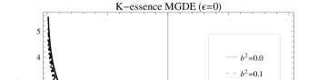
Figure 21: K-essence MGDE scalar field, Eq. (58), versus redshift for different coupling constants $b^{2}$ with $\epsilon=0$. Auxiliary parameters as in Fig. 9.

The evolutionary behavior of this field for different $b^{2}$ and $\epsilon$ is plotted in Figs. 21, 22 and 23. Figures present that the K-essence MGDE scalar field increases during history of the universe.

4.4 Dilaton MGDE

The dilaton scalar field model is also an interesting attempt to explain the origin of DE using string theory. This model appears from a four dimensional effective low energy string action and includes higher order kinetic corrections to the tree level action in low energy effective string theory [94, 95].

For the dilaton scalar field, the pressure and energy density take the forms [94, 95]

$$p_{D}=-\chi+ce^{\lambda\phi}\chi^{2},$$ (59)

$$\rho_{D}=-\chi+3ce^{\lambda\phi}\chi^{2}.$$ (60)

Here $c$ and $\lambda$ are two positive constants and $\chi=\dot{\phi}^{2}/2$ is the dilaton kinetic energy. Therefore, the dilaton EoS parameter reads

$$\omega_{D}=\frac{p_{D}}{\rho_{D}}=\frac{-1+ce^{\lambda\phi}\chi}{-1+3ce^{\lambda\phi}\chi}.$$ (61)

Identifying Eq. (12) with (61) reduces to

$$ce^{\lambda\phi}\chi=\frac{2+\gamma-\frac{\Omega_{k}}{3}+\frac{\gamma-1}{\Omega_{D}}\Big{(}1+\frac{\Omega_{k}}{3}\Big{)}+2b^{2}\Big{(}\frac{1+\Omega_{k}}{\Omega_{D}}\Big{)}-\Omega_{D}+3\epsilon(\Omega_{D}-\gamma-1)}{4+\gamma-\Omega_{k}+\frac{\gamma-1}{\Omega_{D}}(3+\Omega_{k})+6b^{2}\Big{(}\frac{1+\Omega_{k}}{\Omega_{D}}\Big{)}-\Omega_{D}+9\epsilon(\Omega_{D}-\gamma-1)}.$$ (62)

Using $\chi=\dot{\phi}^{2}/2$ one can take the integral of above equation with respect to $a$. The result yields

$$\phi(a)=\frac{2}{\lambda}\ln\left\{e^{\frac{\lambda\phi(a_{i})}{2}}+\delta\int^{a}_{a_{i}}(\Omega_{D}+\gamma-1)\right.~{}~{}~{}~{}~{}~{}~{}~{}~{}~{}~{}~{}~{}~{}~{}~{}~{}~{}~{}~{}~{}~{}~{}~{}~{}~{}~{}~{}~{}~{}~{}~{}~{}~{}~{}~{}~{}~{}~{}~{}~{}~{}~{}~{}~{}~{}~{}~{}~{}~{}~{}~{}~{}~{}~{}~{}~{}~{}~{}~{}~{}~{}~{}~{}~{}~{}$$

$$\left.\times\ \left[\frac{4+2\gamma-\frac{2\Omega_{k}}{3}+2\Big{(}\frac{\gamma-1}{\Omega_{D}}\Big{)}\Big{(}1+\frac{\Omega_{k}}{3}\Big{)}+4b^{2}\Big{(}\frac{1+\Omega_{k}}{\Omega_{D}}\Big{)}-2\Omega_{D}+6\epsilon(\Omega_{D}-\gamma-1)}{4+\gamma-\Omega_{k}+\Big{(}\frac{\gamma-1}{\Omega_{D}}\Big{)}(3+\Omega_{k})+6b^{2}\Big{(}\frac{1+\Omega_{k}}{\Omega_{D}}\Big{)}-\Omega_{D}+9\epsilon(\Omega_{D}-\gamma-1)}\right]^{\frac{1}{2}}~{}\frac{{\rm d}a}{a}\right\},$$ (63)

where $\delta=\frac{3M_{p}^{2}\lambda}{2\alpha\sqrt{c}}$. In Figs. 24, 25 and 26, variation of the dilaton MGDE scalar field, Eq. (63), is illustrated for different $b^{2}$ and $\epsilon$. Figures clear that the scalar field of the dilation MGDE model behaves like the K-essence one (see Figs. 21, 22 and 23).

5 Conclusions

Here we studied the Veneziano MGDE model in the framework of Einstein’s gravity. We considered a spatially non-flat FRW universe filled with interacting viscous MGDE and DM. We derived a differential equation governing the evolution of the MGDE density parameter and solved it numerically. We also obtained the EoS parameter of the interacting viscous MGDE and the deceleration parameter of the universe. Moreover, using the linear perturbation theory we investigated the evolution of growth of structure in our model. Furthermore, using a correspondence between the interacting viscous MGDE and quintessence, tachyon, K-essence and dilaton scalar field models of DE we reconstructed the dynamics $\phi$ and potentials $V(\phi)$ of the aforementioned scalar field models according to the evolution of the MGDE density. Our numerical results show the following.

(i) The MGDE density parameter $\Omega_{D}$ for a given coupling constant $b^{2}$, increases when the time increases. The evolutionary behavior of $\Omega_{D}$ is independent of viscosity.

(ii) The variation of the deceleration parameter $q$ shows that the universe transitions from an early matter dominant epoch to the de Sitter era in the future, as expected. Also $q$ like $\Omega_{D}$ does not depend on viscosity.

(iii) The EoS parameter $\omega_{D}$ of the MGDE model in the absence of viscosity ($\epsilon=0$), varies from the quintessence phase to the phantom regime. Whereas in the absence of interaction ($b^{2}=0$), it behaves like the freezing quintessence model. The interaction and viscosity have opposite effects on $\omega_{D}$.

(iv) The evolution of DM density perturbation $\delta_{\rm m}$ in the presence of interaction shows a suppression of growth of structure. Since the DM density is lower in the past relative to the non-interacting case, leading to a suppression of growth of structure. Here the viscosity constant $\epsilon$ does not affect $\delta_{\rm m}$, because the DM has not the viscosity properties in our model.

(v) The quintessence and tachyon MGDE scalar fields for a given $b^{2}$ or $\epsilon$, increase during history of the universe. For a given redshift, they decrease and increase with increasing $b^{2}$ and $\epsilon$, respectively. The potentials of the quintessence and tachyon MGDE models for a given $b^{2}$ or $\epsilon$, decrease with increasing the time. The interaction and viscosity have opposite effects on both the scalar fields and potentials of the aforementioned models.

(vi) The K-essence and dilaton MGDE scalar fields for a given $b^{2}$ or $\epsilon$ increase during history of the universe.

Acknowledgements

The authors thank the unknown referees for very valuable comments. The work of K. Karami has been supported financially by Center for Excellence in Astronomy & Astrophysics of Iran (CEAAI-RIAAM), under research project No. 1/3076.

Figure 1: MGDE density parameter, Eq. (15), versus redshift for different coupling constants $b^{2}$. Auxiliary parameters are $\Omega_{k_{0}}=0.01$, $\Omega_{D_{0}}=0.76$ and $\gamma=1.105$ [41].

Figure 2: Deceleration parameter, Eq. (14), versus redshift for different coupling constants $b^{2}$. Auxiliary parameters as in Fig. 1.

Figure 3: EoS parameter of MGDE, Eq. (12), versus redshift for different coupling constants $b^{2}$ with $\epsilon=0$. Auxiliary parameters as in Fig. 1.

Figure 5: Same as Fig. 3 for different coupling $b^{2}$ and viscosity $\epsilon$ constants.

Figure 6: Growth factor of DM, Eq. (33), versus redshift for different coupling constants $b^{2}$. Auxiliary parameters are $\Omega_{k_{0}}=0.01$, $\Omega_{D_{0}}=0.76$, $\gamma=1.105$ [41] and $f_{0}=0.473$ [41]. Legend as in Fig. 1.

Figure 7: Dimensionless DM density perturbation, Eq. (36), versus redshift for different coupling constants $b^{2}$. Legend and auxiliary parameters as in Fig. 6.

Figure 8: DM density parameter, $\Omega_{\rm m}=1+\Omega_{k}-\Omega_{D}$, versus redshift for different coupling constants $b^{2}$. Legend and auxiliary parameters as in Fig. 1.

Figure 9: Quintessence MGDE scalar field, Eq. (45), versus redshift for different coupling constants $b^{2}$ with $\epsilon=0$. Auxiliary parameters are $\Omega_{k_{0}}=0.01$, $\Omega_{D_{0}}=0.76$, $\gamma=1.105$ [41] and $\phi(1)=0$.

Figure 10: Same as Fig. 9 for different viscosity constants $\epsilon$ with $b^{2}=0$.

Figure 11: Same as Fig. 9 for different coupling $b^{2}$ and viscosity $\epsilon$ constants.

Figure 12: Quintessence MGDE potential, Eq. (43), versus redshift for different coupling constants $b^{2}$ with $\epsilon=0$. Auxiliary parameter as in Fig. 9.

Figure 13: Same as Fig. 12 for different viscosity constants $\epsilon$ with $b^{2}=0$. Auxiliary parameters as in Fig. 9.

Figure 14: Same as Fig. 12 for different coupling $b^{2}$ and viscosity $\epsilon$ constants. Auxiliary parameters as in Fig. 9.

Figure 15: Tachyon MGDE scalar field, Eq. (52), versus redshift for different coupling constants $b^{2}$ with $\epsilon=0$. Auxiliary parameters as in Fig. 9.

Figure 16: Same as Fig. 15 for different viscosity constants $\epsilon$ with $b^{2}=0$.

Figure 17: Same as Fig. 15 for different coupling $b^{2}$ and viscosity $\epsilon$ constants.

Figure 18: Tachyon MGDE potential, Eq. (51), versus redshift for different coupling constants $b^{2}$ with $\epsilon=0$. Auxiliary parameter as in Fig. 9.

Figure 19: Same as Fig. 18 for different viscosity constants $\epsilon$ with $b^{2}=0$.

Figure 20: Same as Fig. 18 for different coupling $b^{2}$ and viscosity $\epsilon$ constants.

Figure 22: Same as Fig. 21 for different viscosity constants $\epsilon$ with $b^{2}=0$.

Figure 23: Same as Fig. 21 for different coupling $b^{2}$ and viscosity $\epsilon$ constants.

Figure 24: Dilaton MGDE scalar field, Eq. (63), versus redshift for different coupling constants $b^{2}$ with $\epsilon=0$. Auxiliary parameters are $\Omega_{k_{0}}=0.01$, $\Omega_{D_{0}}=0.76$, $\gamma=1.105$ [41], $\phi(1)=0$ and $\delta=\frac{3M_{p}^{2}\lambda}{2\alpha\sqrt{c}}=1$.

Figure 25: Same as Fig. 24 for different viscosity constants $\epsilon$ with $b^{2}=0$.

Figure 26: Same as Fig. 24 for different coupling $b^{2}$ and viscosity $\epsilon$ constants.

References

- [1] S. Perlmutter, et al., Astrophys. J. 483, 565 (1997).
- [2] S. Perlmutter, et al., Nature 391, 51 (1998).
- [3] S. Perlmutter, et al., Astrophys. J. 517, 565 (1999).
- [4] A.G. Riess, et al., Astrophys. J. 607, 665 (2004).
- [5] A.G. Riess, et al., Astrophys. J. 659, 98 (2007).
- [6] C. Bennett, et al., Astrophys. J. Suppl. 148, 1 (2003).
- [7] D.N. Spergel, et al., Astrophys. J. Suppl. 148, 175 (2003).
- [8] D.N. Spergel, et al., Astrophys. J. Suppl. 170, 377 (2007).
- [9] E. Hawkins, et al., Mon. Not. Roy. Astron. Soc. 346, 78 (2003).
- [10] M. Tegmark, et al., Phys. Rev. D 69, 103501 (2004).
- [11] S. Cole, et al., Mon. Not. Roy. Astron. Soc. 362, 505 (2005).
- [12] D.J. Eisenstein, et al., Astrophys. J. 633, 560 (2005).
- [13] B. Jain, A. Taylor, Phys. Rev. Lett. 91, 141302 (2003).
- [14] V. Sahni, A.A. Starobinsky, Int. J. Mod. Phys. D 9, 373 (2000).
- [15] T. Padmanabhan, Phys. Rep. 380, 235 (2003).
- [16] P.J.E. Peebles, B. Ratra, Rev. Mod. Phys. 75, 559 (2003).
- [17] S. Weinberg, Rev. Mod. Phys. 61, 1 (1989).
- [18] F.R. Urban, A.R. Zhitnitsky, Phys. Rev. D 80, 063001 (2009).
- [19] F.R. Urban, A.R. Zhitnitsky, Phys. Lett. B 688, 9 (2010).
- [20] N. Ohta, Phys. Lett. B 695, 41 (2011).
- [21] E. Witten, Nucl. Phys. B 156, 269 (1979).
- [22] G. Veneziano, Nucl. Phys. B 159, 213 (1979).
- [23] K. Kawarabayashi, N. Ohta, Nucl. Phys. B 175, 477 (1980).
- [24] C. Rosenzweig, J. Schechter, C.G. Trahern, Phys. Rev. D 21, 3388 (1980).
- [25] P. Nath, R.L. Arnowitt, Phys. Rev. D 23, 473 (1981).
- [26] M.M. Forbes, A.R. Zhitnitsky, Phys. Rev. D 78, 083505 (2008).
- [27] A.R. Zhitnitsky, Phys. Rev. D 82, 103520 (2010).
- [28] A.R. Zhitnitsky, Phys. Rev. D 84, 124008 (2011).
- [29] B. Holdom, Phys. Lett. B 697, 351 (2011).
- [30] R.G. Cai, Z.L. Tuo, H.B. Zhang, Q. Su, Phys. Rev. D 84, 123501 (2011).
- [31] E. Ebrahimi, A. Sheykhi, Phys. Lett. B 705, 19 (2011).
- [32] E. Ebrahimi, A. Sheykhi, Int. J. Mod. Phys. D 20, 2369 (2011).
- [33] A. Khodam-Mohammadi, et al., Mod. Phys. Lett. A 27, 1250100 (2012).
- [34] K. Karami, A. Abdolmaleki, arXiv:1202.2278.
- [35] K. Saaidi, arXiv:1202.4097.
- [36] K. Saaidi, A. Aghamohammadi, B. Sabet, arXiv:1203.4518.
- [37] A. Sheykhi, M. Sadegh Movahed, Gen. Relativ. Gravit. 44, 449 (2012).
- [38] A. Sheykhi, A. Bagheri, Europhys. Lett. 95, 39001 (2011).
- [39] A. Sheykhi, M. Sadegh Movahed, E. Ebrahimi, Astrophys. Space Sci. 339, 93 (2012).
- [40] A. Rozas-Fernandez, Phys. Lett. B 709, 313 (2012).
- [41] R.G. Cai, Z.L. Tuo, Y.B. Wu, Y.Y. Zhao, Phys. Rev. D 86, 023511 (2012).
- [42] A.R. Zhitnitsky, arXiv:1112.3365.
- [43] M. Maggiore, Phys. Rev. D 83, 063514 (2011).
- [44] M. Maggiore, et al., Phys. Lett. B 704, 102 (2011).
- [45] E.J. Copeland, M. Sami, S. Tsujikawa, Int. J. Mod. Phys. D 15, 1753 (2006).
- [46] A. Ali, M. Sami, A.A. Sen, Phys. Rev. D 79, 123501 (2009).
- [47] J.P. Wu, D.Z. Ma, Y. Ling, Phys. Lett. B 663, 152 (2008).
- [48] X. Zhang, Phys. Rev. D 74, 103505 (2006).
- [49] X. Zhang, Phys. Lett. B 648, 1 (2007).
- [50] J. Zhang, X. Zhang, H. Liu, Phys. Lett. B 651, 84 (2007).
- [51] X. Zhang, Phys. Rev. D 79, 103509 (2009).
- [52] L.N. Granda, A. Oliveros, Phys. Lett. B 671, 199 (2009).
- [53] K. Karami, J. Fehri, Phys. Lett. B 684, 61 (2010).
- [54] K. Karami, M.S. Khaledian, M. Jamil, Phys. Scr. 83, 025901 (2011).
- [55] J. Zhang, X. Zhang, H. Liu, Eur. Phys. J. C 54, 303 (2008).
- [56] A. Sheykhi, Phys. Lett. B 682, 329 (2010).
- [57] K. Karami, et al., Phys. Lett. B 686, 216 (2010).
- [58] K. Karami, A. Abdolmaleki, Astrophys. Space Sci. 330, 133 (2010).
- [59] W. Zimdahl, D. Pavón, L.P. Chimento, Phys. Lett. B 521, 133 (2001).
- [60] W. Zimdahl, D. Pavón, Gen. Relativ. Gravit. 35, 413 (2003).
- [61] L.P. Chimento, et al., Phys. Rev. D 67, 083513 (2003).
- [62] O. Bertolami, F. Gil Pedro, M. Le Delliou, Gen. Relativ. Gravit. 41, 2839 (2009).
- [63] E. Abdalla, L.R. Abramo, L. Sodre, B. Wang, Phys. Lett. B 673, 107 (2009).
- [64] T.R. Jaffe, et al., Astrophys. J. 629, L1 (2005).
- [65] V. Folomeev, V. Gurovich, Phys. Lett. B 661, 75 (2008).
- [66] I. Brevik, Phys. Rev. D 65, 127302 (2002).
- [67] I. Brevik, O. Gorbunova, Gen. Relativ. Gravit. 37, 2039 (2005).
- [68] I. Brevik, O. Gorbunova, Eur. Phys. J. C 56, 425 (2008).
- [69] I. Brevik, O. Gorbunova, D.S. Gomez, Gen. Relativ. Gravit. 42, 1513 (2010).
- [70] O. Bertolami, F. Gil Pedro, M. Le Delliou, Phys. Lett. B 654, 165 (2007).
- [71] L.L. Honorez, et al., JCAP 09, 029 (2010).
- [72] H. Kim, H.W. Lee, Y.S. Myung, Phys. Lett. B 632, 605 (2006).
- [73] L. Amendola, Phys. Rev. D 62, 043511 (2000).
- [74] E.E.O. Ishida, et al., Astropart. Phys. 28, 547 (2008).
- [75] R.R. Caldwell, E.V. Linder, Phys. Rev. Lett. 95, 141301 (2005).
- [76] T. Padmanabhan, Structure formation in the universe (Cambridge University Press, 1993).
- [77] C. Feng, B. Wang, E. Abdalla, R.K. Su, Phys. Lett. B 665, 111 (2008).
- [78] G. Caldera-Cabral, R. Maartens, B.M. Schaefer, JCAP 07, 027 (2009).
- [79] V. Sahni, A.A. Starobinsky, Int. J. Mod. Phys. D 15, 2105 (2006).
- [80] B. Ratra, J. Peebles, Phys. Rev. D 37, 321 (1988).
- [81] R.R. Caldwell, R. Dave, P.J. Steinhardt, Phys. Rev. Lett. 80, 1582 (1998).
- [82] R.R. Caldwell, Phys. Lett. B 545, 23 (2002).
- [83] A. Sen, JHEP 10, 008 (1999).
- [84] A. Sen, JHEP 04, 048 (2002).
- [85] A. Sen, JHEP 07, 065 (2002).
- [86] E.A. Bergshoeff, et al., JHEP 05, 009 (2000).
- [87] T. Padmanabhan, Phys. Rev. D 66, 021301 (2002).
- [88] T. Padmanabhan, T.R. Choudhury, Phys. Rev. D 66, 081301 (2002).
- [89] T. Chiba, T. Okabe, M. Yamaguchi, Phys. Rev. D 62, 023511 (2000).
- [90] C. Armendáriz-Picón, V. Mukhanov, P.J. Steinhardt, Phys. Rev. Lett. 85, 4438 (2000).
- [91] C. Armendáriz-Picón, V. Mukhanov, P.J. Steinhardt, Phys. Rev. D 63, 103510 (2001).
- [92] C. Armendáriz-Picón, T. Damour, V. Mukhanov, Phys. Lett. B 458, 209 (1999).
- [93] J. Garriga, V. Mukhanov, Phys. Lett. B 458, 219 (1999).
- [94] M. Gasperini, F. Piazza, G. Veneziano, Phys. Rev. D 65, 023508 (2002).
- [95] N. Arkani-Hamed, et al., JCAP 04, 001 (2004).